A Hybrid SAR Autofocus Technique by Two Methods of
Sub-Aperture Estimation and Iterative Golden Section Search
Boyeon Koh*, Sanghyouk Choi, and Joohwan Chun
Abstract—In a real airborne synthetic aperture radar (SAR), its major phase errors are usually composed of two categories, such as slow-time varying phase errors (less than several cycles of change in phase during synthetic aperture time) and fast-time varying phase errors (otherwise, including wide band random) according to the motion of aircraft. If the fast errors are no more negligible compared to the slow errors, they should be estimated and then compensated accurately to obtain a well focused image. However, it is not proper to estimate all phase errors at the same time like conventional autofocus techniques because the estimation of the fast-time varying phase errors are seriously affected by blurring in image due to the slow-time varying phase errors. In this paper, we presents an accurate hybrid phase estimation technique using two independent estimation stages of sub-aperture and an iterative golden section search method, which has advantages over several existing methods, because of its better estimation accuracy and less sensitive to the quality of extracted range bins as well as requiring less computation time. The performance of our method is illustrated by simulations of point targets and an experiment with real SAR data.
1. INTRODUCTION
Autofocus techniques for synthetic aperture radar (SAR) have been a major concern, and many attempts have been made to improve their performance for real SAR applications. Autofocus techniques are generally categorized into two types according to the estimation method: parametric or non-parametric. In parametric methods [1, 2] phase errors are approximated by an appropriate model with specific parameters, whereas non-parametric method [3–5] do not require a phase error model, thus allowing us to estimate a wide variety of phase errors. Non-parametric methods such as the phase gradient algorithm (PGA) [3, 4], the eigenvector method (EVM) [6], the weighted least square (WLS) [7], and the successive parameter adjustment (SPA) [8] are widely used owing to their good performance compared to the computation time required. However, the performance of non-parametric methods, which require range bins for estimation, seriously depends on the quality of the extracted range bins from an unfocused image. Studies have been conducted on the selection of good range bins and on an iterative selection method during estimations [9, 10] to overcome the above constraint. Furthermore, if the fast-varying phase errors such as wideband random (WBR) phase errors are serious and should be removed for a well-focused image as often experienced in low-altitude airborne SAR, a gradient-based non-parametric method such as PGA is not proper to use for an accurate estimation because the calculations of gradient are severely affected by the WBR phase errors. The SPA method modeling unknown phase errors using orthogonal polynomial (Legendre) shows a good performance in case of the polynomial type of phase errors. However, it is not proper to apply in case of the WBR phase errors because it is insufficient to approximate the phase errors with finite polynomials. A non-gradient-based method [11] was proposed to cope with the WBR phase errors for inverse SAR (ISAR) applications; however, it requires a considerable
Received 19 June 2014, Accepted 14 August 2014, Scheduled 22 August 2014 * Corresponding author: Boyeon Koh ([email protected]).
amount of computation time for the case of SAR, which requires a much longer synthetic aperture time (SAT) than ISAR.
In this paper, we propose a hybrid estimation technique to provide an accurate estimation for both the slow-time varying (STV) errors and the WBR phase errors. It is assumed that the extracted range bin contains a dominant point like scatterer (target) with some strong clutters, similar to a real SAR environment. The proposed method consists of two estimation stages, the first for the estimation of STV phase errors and the second for the estimation of all errors, including any residual errors remaining after the first stage. A sub-aperture estimation method is utilized for the first stage, and then we adopt an iterative golden section search (IGSS) method for the second stage to ensure an efficient computation time while maintaining an accurate estimation. Simulations and an experiment with real SAR data illustrate the performance of our method.
2. FIRST STAGE: ESTIMATION OF THE STV PHASE ERRORS
2.1. Model of a Single Range Bin for Phase Estimation
The single range bin extracted from an unfocused image can be modeled as
g(t) =
a0ejω0t+ C
c=1
acejωct
ejϕ(t), a
0 > ac. (1)
Here,tindicates the azimuth time;C denotes the number of non-negligible clutters (NNCs) which cannot be neglected in comparison to the dominant target. Additionally, a0 and ac, and ωc and ωc are
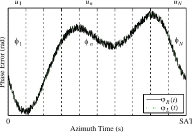
respectively the amplitudes and angular frequencies of the target and NNCs. The overall phase error is denoted as ϕ(t), and it is simply assumed to have two types of errors, defined as ϕL(t) for the STV phase error and ϕR(t) for the WBR phase error (see Figure 1, for example). The purpose of the first
stage of our method is to estimate ϕL(t) in (1) and compensated it prior to proceeding to the second
stage for an accurate estimation.
2.2. Estimation of the ϕL(t) by Sub-Aperture Method
As in other sub-aperture methods [12], the SAT is divided into N non-overlapping segments (u1, . . . , uN), as shown in Figure 1. Thenth segment phase error ϕL,n(t) is modeled as
ϕL,n(t) =ejφn(t,βn), φn(t,βn) = Q
q=0
βn,qtq. (2)
Here, Q indicates the polynomial order of the model, and βn is the parameter to be estimated. We
definez(t) =ej∠g(t) by (1) with zk being the sample ofz(t=tk). All zk values are assumed to have an
equal length ofM, and each segment thus has M datum pairs (ti, zi) with the expression of ˆzi = (ˆxi,yˆi)
0 SAT
Azimuth Time (s)
Phase Error (rad)
u1 un uN
1 n N
(t) (t)
ϕ ϕ
φ φ φ
R L
as the estimation ofzi = (xi, yi). The goal is to optimize theβnparameters of theφn(t,βn) model such that the sum of the squares of the error E(β) is minimized (the subscript ‘n’ is omitted hereafter for simplicity):
E(β) =
M
i=1
|zi−zˆi|2= M
i=1
zi−ejφ(ti,β)=
M
i=1
[xi−cos (φ(ti,β))]2+ [yi−sin (φ(ti,β))]2
. (3)
The normal equation is obtained by a linearization of ˆzi around the pre-estimatedβl−1 via a Taylor series expansion of the first order, as follows:
ˆ
xi
ti,βl ≈xˆi
ti,βl−1 +
Q
s=0
∂xˆiti,βl−1
∂βs
βsl−βl−1 s = ˆxi
ti,βl−1 +
Q
s=0
gisΔβs
ˆ
yi
ti,βl ≈yˆi
ti,βl−1 +
Q
s=0
∂yˆiti,βl−1
∂βs
βsl −βl−1 s = ˆyi
ti,βl−1 +
Q
s=0
hisΔβs
(4)
where gis= ∂β∂xˆi
s, his =
∂yˆi
∂βs, Δβs=β l
s−βsl−1.
Taking the gradient of (3) with respect toβq, (q= 0,1,2 ) and using the relationships in (4) results in
∂E(β)
∂βq = M
i=1
∂E
(β)
∂xˆi ·
∂xˆi
∂βq +
∂E(β)
∂yˆi ·
∂yˆi
∂βq = 2 M i=1
xi−xˆi− Q
s=0
gisΔβs
giq+
yi−yˆi− Q
s=0
hisΔβs hiq = 2 M i=1
Δxi− Q
s=0
gisΔβs
giq+
Δyi− Q
s=0
hisΔβs
hiq
.
Then normal equation is obtained as
M i=1 Q s=0
(gisgiq+hishiq)Δβs= M
i=1
(Δxigiq+ Δyihiq). (5)
In vector notation, (5) becomes (here,T indicates transpose)
GTG+HTH Δβ=GTΔx+HTΔy.
In this paper, the normal equation is solved by the LMA (Levenberg-Marquardt Algorithm) with the damping parameter λ[13] as
GTG+HTH+λ·diag
GTG+HTH Δβ=GTΔx+HTΔy. (6)
2.3. Good Initial Guess of βn
Like other iterative methods, a good initial guess of β0 leads to a better optimal solution. When a quadratic model is used, a good β0 can be determined by an efficient search strategy based on the following characteristics:
1)β2 only dominates the entropy of the image; thus,β20 is determined by a search for a value ofβ2 that
minimizes the entropy function defined below
H[β2] = M−1
k=0
|G(k, β2)|ln [|G(k, β2)|],
G(k, β2) = M−1
m=0
zme−j2πkmM e−jβ2m2, β20 = arg min
2)β1causes a shift in the image domain according to the value ofβ1; thus,β10is determined by measuring
the amount of shift in|G(k;β20)|.
3) β00 is finally determined by a search for a value of β0 that minimizes the error cost function with the
previously determined initial estimates of β20 and β10, as defined below
E(β0;β10, β20) = M
i=1
|zi−zˆi|2
β0
0 = arg minβ 0
Eβ0;β10, β20
.
In our experiment,βn was sufficiently obtained by solving (6) within dozens of iterations with feasible values ofβ0.
3. SECOND ESTIMATION STAGE FOR THE WBR PHASE ERRORS
After the compensation ofϕL(t), the second stage for an accurate estimation of the WBR phase errors
is performed to create a full focused image. Unlike ϕL(t), ϕR(t) requires an exhaustive search time to
find a global optimum estimation; therefore, near-optimal estimation techniques are usually employed. Entropy minimization techniques have been proposed for ISAR applications [11, 14]. The SSA [11] is one of effective methods to estimate the WBR phase errors in accurate. However, it requires a considerable amount of computation time when applied to real SAR applications. Therefore, we adopt an iterative golden section search (IGSS) method which requires much less computation time over the SSA. The IGSS method is based on the concept of a golden section search [15] with entropy minimization in the image domain, as with the SSA. The utilization of golden section search for the estimation of phase errors was firstly proposed in [8], which finds optimum coefficients of Legendre polynomials. This paper utilizes the golden section search for direct estimation of all phase errors at every azimuth positions in order to compensate the WBR phase errors in accurate. One factor to consider is that the entropy function in the IGSS method must satisfy the unimodal condition within the search section. Fortunately, when the entire search section is divided into sub-sections, this condition can be satisfied in each sub-section. The final solution will then be obtained by the selection of the best result between two sub-sections with minimum entropy. In our experiment, the condition is satisfied by dividing the entire search section
L: [−π, π] into two the sub-sections ofL−: [−π,0] andL+: [0, π], after which a better optimal solution is attainable through GSS iterations. For a clear explanation of our method, definitions of the variables and functions are necessary. After compensation of STV phase error ϕL(t), we define ˜g(t), ˜gn, andψn
as follows:
˜
g(t) =g(t)e−jϕL(t)
˜
gn= ˜g(t=tn)
ψn=ϕR(t=tn), n= 0∼NT −1.
(7)
Here, NT indicates the number of samples of ˜gn, and ψn is the WBR phase error att =tn. The
function of the GSS method is defined as [ ˆψp, hp] =GDN(L, H( ˆψ, ψp,Δ)), whereLindicates the search
section, ˆψp andhp are the search result and matching minimum entropy att=tp, ˆψ is the vector array
of ˆψ= [ ˆψ0. . .ψˆNT−1], and Δ is the tolerance parameter of the GSS method. Additionally, the entropy
functionH( ˆψ, ψp) used in our method is defined below similar to the cost function used in [11, 16]
Hψˆ, ψp ≡
NT−1
k=0
F˜k; ˆψ, ψp lnF˜k; ˆψ, ψp
˜
Fk; ˆψ, ψp ≡ NT−1
n=0
˜
fne−j 2πkn
NT
(8)
With all of the above definitions, an overall processing flow diagram of the IGSS method is depicted in Figure 2. Here, l and p are the indices of iteration andNiter denotes the maximum iteration number,
andis the threshold for termination. The parameters Δ anddo not need to be fixed but instead can vary with the iterations like Δ(l) and (l) to obtain a better solution.
Figure 2. Processing flow diagram of the IGSS method.
-5 -4 -3 -2 -1 0 1 2 3 4 5
0 0.2 0.4 0.6 0.8 1
Azimuth Time (sec)
-5 -4 -3 -2 -1 0 1 2 3 4 5
0 0.2 0.4 0.6 0.8 1
Azimuth Time (sec)
-5 -2.5 0 2.5 5
-20 -10 0 10 20
Azimuth Time (sec)
Phase Error (rad)
-5 -2.5 0 2.5 5
Azimuth Time (sec)
(a) (b)
(c) (d)
-2 -1 0 1 2
Phase Error (rad)
Normalized RCS Normalized RCS
Figure 3. Two extracted range bins and phase errors. (a) Uncorrupted original range bin for target #1. (b) Uncorrupted original range bin for target #2. (c) STV phase error ϕL(t). (d) WBR phase errorϕR(t).
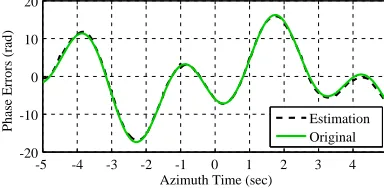
-5 -4 -3 -2 -1 0 1 2 3 4 5
Azimuth Time (sec)
Estimation Original -20
-10 0 10 20
Phase Errors (rad)
4. SIMULATION AND REAL DATA PROCESSING
4.1. Simulations with Point Targets with NNCs
Simulations with point targets were performed to illustrate the performance of the proposed method. We assumed that two extracted range bins contained some NNCs and that the phase errorϕ(t) consisted of both STV and WBR phase errors, as shown in Figure 3.
The result of the first stage is given in Figure 4, which shows that a good approximation of
ϕL(t) is achieved by the sub-aperture estimation. The final results of the proposed method and other
1 1000 2000 1 1000 2000
1 1000 2000 1 1000 2000 1 1000 2000 1 1000 2000
1 1000 2000 1 1000 2000 1 1000 2000 1 1000 2000
1 1000 2000 1 1000 2000 1 1000 2000 1 1000 2000
1 1000 2000 1 1000 2000
0 1.0
0 1.0
0 1.0
0 1.0
0 1.0
0 1.0
0 1.0
0 1.0
0 1.0
0 1.0
0 1.0
0 1.0
0 1.0
0 1.0
0 1.0
0 1.0 (a)
(b) (c)
(d) (e)
(f) (g)
(h)
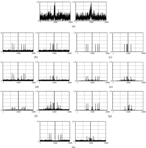
conventional methods are presented in Figure 5. The defocused two images by ϕ(t) are given in Figure 5(a). After compensation of the STV phase errors, focused (but not fully) images are obtained, as shown in Figure 5(b). The final images after second stage with the IGSS method are presented in Figure 5(c), which completely restores the original range bins without any degradation or spurious
1000 2000 3000 4000 5000
Range Bin Length (pixel) IGSS
SSA
0 20 40 60 80 100 120 140
Computation Time (min)
Figure 6. The computation time of the IGSS and SSA.
(a)
(b) (c)
(d) (e)
targets. In contrast, all other conventional methods which are sensitive to the quality of the extracted range bins show some loss in the amplitude (radar cross section) of each NNCs. Also, many spurious targets appear, as shown in Figure 5(d) for the PGA, 5(e) for the EVM, Figure 5(f) for the WLS, and Figure 5(h) for the SPM. The autofocus techniques such as the PGA and the SPM show that lots of residual phase errors still remain in the processed images as the WBR phase errors are difficult to be estimated using these techniques. To investigate the effectiveness of the first stage in the proposed method, Direct estimation of both ϕL(t) and ϕR(t) via the SSA was performed. The Figure 5(g)
illustrates that the blurring effect of ϕL(t) leads to an inaccurate estimation of the total phase error
of ϕ(t) and that it should be compensated before the second stage. The computation efficiency of the IGSS was also tested and compared to that of the SSA. The test was performed on a PC equipped with an Intel(R) Xeon X5460 processor, and we measured each processing time for the IGSS and SSA to estimate the WBR phase errors, which were intentionally added to an uncorrupted range bin. Figure 6 shows that the IGSS requires much less computation time than the SSA and that more efficiency is achieved as the length of the range bin increases.
4.2. Experiment with a Real SAR Data
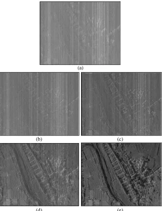
The processing result with a real SAR siginal data is given in Figure 7. The resolution is 1 m, and the scene size is 2 km×2 km in terms of the range and azimuth. The operation altitude was 10,000 feet, and the weather condition of that day was not good for image acquisition, thus the phase errors of STV and WBR were serious caused by the turbulence of air. The blurring image by the phase errors is shown in Figure 7(a). The processing results of the PGA and the SPA are given in Figures 7(b) and 7(c), which illustrate that the PGA and the SPA enable us to estimate the STV phase errors but that they cannot sufficiently estimate the WBR phase errors, as many random phase errors remain in the processed images. However, the SPA is better than the PGA because some of the WBR phase errors can be approximated with high order Legendre polynomials. The result processing with the SSA is also presented in Figures 7(d), which illustrates that only the SSA method without the first compensation of
ϕL(t) is not sufficient to provide an accurate estimation of all phase errorsϕ(t), as discussed in the section
on point target simulations. The performance of the proposed method is presented in Figure 7(e), which demonstrates that an accurate estimation of both STV and WBR phase errors is achieved such that well focused image is restored without serious degradation. In order to check the performance of each method objectively, an image quality parameter of contrast (CNT = variance/mean) was calculated, and the best value of contrast is obtained by the the proposed method as shown in Figure 7(e).
5. CONCLUSIONS
From the simulations and real SAR image processing assessments, we conclude that the proposed method can provide better performance than several existing autofocus methods in terms of the estimation accuracy and computation time. We illustrate that our method can effectively be applied to the case of low-altitude airborne SAR operations where the WBR phase errors are not trivial.
REFERENCES
1. Samczynski, P. and K. S. Kulpa, “Coherent mapdrift technique,” IEEE Transactions on Geosci. Remote Sens., Vol. 48, No. 3, 1505–1517, 2010.
2. Xu, J., Y. Peng, and X. G. Xia, “Parametric autofocus of SAR imaging — Inherent accuracy limitations and realization,” IEEE Transactions on Geosci. Remote Sens., Vol. 42, No. 11, 2397– 2411, 2004.
3. Wahl, D. E., P. H. Eichel, D. C. Ghiglia, and C. V. Jakowatz, Jr., “Phase gradient autofocus — A robust tool for high resolution phase correction,” IEEE Trans. on Aerosp. Electron. Syst., Vol. 30, No. 3, 827–835, 1994.
5. Kolman, J., “PACE: An autofocus algorithm for SAR,”Proc. Int. Radar Conf., 310–314, Arlington, VA, 2005.
6. Jakowatz, Jr., C. V. and D. E. Wahl, “Eigenvector method for maximum-likelihood estimation of phase errors in synthetic aperture radar imagery,”J. Opt. Soc. Am. A, Vol. 10, No. 12, 2539–2546, 1993.
7. Ye, W., T. S. Yeo, and Z. Bao, “Weighted least-squares estimation of phase errors for SAR/ISAR autofocus,”IEEE Transactions on Geosci. Remote Sens., Vol. 37, No. 5, 2487–2494, 1999.
8. Cho, K. M. and L. H. Hui, “Autofocus method based on successive parameter adjustments for contrast optimization,” US Patent 7 145 496, Dec. 5, 2006.
9. Fu, T., M. G. Gao, and Y. He, “An improved scatter selection method for phase gradient autofocus algorithm in SAR/ISAR autofocus,”IEEE Int. Conf. Neural Network and Signal Processing, 1054– 1057, Dec. 2013.
10. Tang, H., H. Shi, and C. Qi, “Study on improvement of phase gradient autofocus algorithm,”First Int. Workshop on Education Technology and Computer Science ETCS 2009, Vol. 2, 58–61, 2009. 11. Xi, L., L. Guosui, and J. Ni, “Autofocusing of ISAR images based on entropy minimization,”IEEE
Trans. on Aerosp. Electron. Syst., Vol. 35, No. 4, 1240–1252, 1999.
12. Calloway, T. M. and G. W. Donohoe, “Subaperture autofocus for synthetic aperture radar,”IEEE Trans. on Aerosp. Electron. Syst., Vol. 30, No. 2, 617–621, 1994.
13. Wright, N. J. and J. Stagehen, Numerical Optimization, 2nd Edition, Springer, 2006.
14. Wang, J., X. Liu, and Z. Zhou, “Minimum-entropy phase adjustment for ISAR,” IEEE Proc. — Radar Sonar Navigat., Vol. 151, No. 4, 203–209, 2004.
15. Press, W. H., S. A. Teukolsky, W. T. Vetterling, and B. P. Flannery,Numerical Recipes: The Art of Scientific Computing, 3rd Edition, Cambridge University Press, 2007.
16. Kragh, T. J. and A. A. Kharbouch, “Monotonic iterative algorithms for SAR image reconstruction,”