Improvements to Tracking Pedestrians in Video Streams Using a Pre-trained Convolutional Neural Network

(1)

Scholarship@Western

Electronic Thesis and Dissertation Repository

6-10-2016 12:00 AM

Improvements to Tracking Pedestrians in Video Streams Using a

Pre-trained Convolutional Neural Network

Marjan Ramin

The University of Western Ontario

Supervisor

Dr. Jagath Samarabandu

The University of Western Ontario

Graduate Program in Electrical and Computer Engineering

A thesis submitted in partial fulfillment of the requirements for the degree in Master of Engineering Science

Follow this and additional works at: https://ir.lib.uwo.ca/etd Part of the Computer Engineering Commons

Recommended Citation Recommended Citation

Ramin, Marjan, "Improvements to Tracking Pedestrians in Video Streams Using a Pre-trained Convolutional Neural Network" (2016). Electronic Thesis and Dissertation Repository. 3886. https://ir.lib.uwo.ca/etd/3886

This Dissertation/Thesis is brought to you for free and open access by Scholarship@Western. It has been accepted for inclusion in Electronic Thesis and Dissertation Repository by an authorized administrator of

(2)

Target tracking has many applications in various fields. Millions of cameras are being used

globally and people are constantly being watched everywhere. These cameras record over 48

hours of videos weekly which are impossible to be monitored manually. Many applications

have been presented to improve the performance of pedestrian tracking. However, it still has

remained a challenging topic. In this thesis, an automatic method is proposed for multiple

pedestrian tracking. State-of-the-art detection has been combined with a tracking algorithm,

followed by a novel post stage processing to increase the accuracy. Proposed automatic

track-ing system was compared with a state-of-the-art tracktrack-ing algorithm which shows comparable

accuracy when used with the original incomplete ground truth data. It is estimated to offer

bet-ter accuracy with a more accurate ground truth data. The proposed algorithm offers potential

improvements in both true positives as well as false negatives ratio when compared with the

existing algorithm.

(3)

Firstly, I would like to express my sincere gratitude to my advisor Dr. Samarabandu for the

continuous support of my Masters study and related research, for his patience, motivation, and

immense knowledge.

Nobody has been more important to me in the pursuit of this project than my family. I would

like to thank my adorable parents and my lovely sisters, whose love and guidance are with me

in whatever I pursue and were always there for moral and emotional support although lived far

away from me for past two years.

I cannot express enough thanks to my friends for their continued support and encouragement.

I also would like to thank professors at Western who provided me knowledge and guidance.

Last but not least, thank you very much for all the staffin Western University for taking good

care of me.

(4)

Acknowlegements i

Abstract i

Acknowledgements ii

List of Figures v

List of Tables viii

List of Appendices ix

List of Abbreviations x

1 Introduction 1

1.1 Motivation . . . 1

1.2 Contributions . . . 4

1.3 Document Structure . . . 5

2 Background 6 2.1 Object Representation . . . 6

2.2 Feature Selection for Tracking . . . 7

2.2.1 Hand-crafted features . . . 7

2.2.2 Features learned from data . . . 10

2.2.2.1 Deap Learning . . . 11

(5)

2.4 Object Tracking Algorithms . . . 25

2.4.1 Target Representation and Localization . . . 25

2.4.2 Filtering and Data Association . . . 26

3 Methodology 30 3.1 Detection . . . 30

3.2 Visual Tracking . . . 31

3.3 Post Stage Processing . . . 33

3.4 Algorithm and Software Development Steps . . . 35

3.5 Dataset . . . 37

3.6 Evaluation . . . 38

4 Results 43 4.1 Occlusion Handling . . . 48

4.2 In-house Dataset . . . 48

5 Discussion and Future Work 55 5.1 Discussion . . . 55

5.2 Future work . . . 56

Bibliography 58

A MATLAB Implementation 65

Curriculum Vitae 79

(6)

2.1 Object Representation samples [1]. . . 8

2.2 Alex net CNN structure consists of five convolutional layers, three pooling layers, and three fully connected layers which is designed for object detection tasks [2]. . . 13

2.3 Auto Encoder that projects the input to output. . . 14

2.4 Comparing a separator line in a binary space using different models. Black dots represent class 1 and blue dots represent class 2. Blue line indicates the class boundary found by various algorithms. [3]. . . 15

2.5 Neural net before and after dropout [4]. . . 19

2.6 Target Presentation Samples. . . 27

2.7 Linear Programming method for multi-object tracking [5] The image shows the xandycoordinates of bounding boxes of two moving objects. The global optimum is found using ILP although objects have overlaps in some occasions. 28 2.8 Representing ILP in a flow network where the shortest path is used to find the best possible track for each pedestrian. . . 29

3.1 R-CNN structure 3.1 . . . 31

3.2 This figure shows tracked pedestrians with specified label numbers as well as births and deaths of tracks of individual pedestrians. . . 32

3.3 Limitation of simply using euclidian distance to join the broken tracks. . . 34

3.4 Flowchart of the presented Post Stage Processing . . . 40

3.5 Sample images from ETHZ Dataset. . . 41

(7)

3.7 Sample image from my dataset, showing pedestrians in distance. . . 42

4.1 (a) represents a specific frame in the tracking results of the proposed method

in this thesis. (b) is the same frame which shows the result of tracking method

presented by Pirsiavash et al. [6], and (c) shows bounding boxes annotated in

the same frame of the original video sequence. . . 44

4.2 Left image shows the annotated bounding boxes in the original video sequences,

and the image in right represents the results of proposed method. Bounding

boxes 134 and 413 are missclassified although they are truly pedestrians. . . 47

boxes 231 and 439 are missclassified and one pedestrian could not be detected

and tracked. . . 48

boxes 547 and 684 are missclassified. . . 49

boxes 135 and 51 are missclassified. . . 49

boxes 244, 312, and another bounding box are missclassified. . . 50

and the image in right represents the results of proposed method. It shows that

the proposed method in some cases is more precise than the annotations in the

original video sequence. . . 50

(8)

video sequences. . . 51

4.9 Comparing the original video sequence, on the left, with results achieved by the

proposed method, on the right. Bounding boxes 362 and 145 are missclassified

although they are truly pedestrians. . . 51

4.10 Comparing the original video sequence, on the left, with results achieved by the

proposed method, on the right. Bounding boxes 231 and 684 are missclassified

although they are truly pedestrians. . . 52

4.11 This is a sample of equality in the pedestrians detected in both original video

sequences and results of the proposed method. . . 52

4.12 A sequence of frames, starting from right to left, in which a pedestrian is

oc-cluded with an object. The proposed method handled this problem. . . 53

4.13 Partial Occlusion Handling . . . 53

4.14 These frames show a part of the results of the second experiment presented in

this study. The same approach as the first experiment on ETHZ dataset is used

using same values for all the parameters like Euclidian distance threshold. . . . 54

(9)

4.1 This table shows the actual True Positive (TP), False Positive (FP), False

Neg-ative (FN), and True NegNeg-ative (TN) values of the final tracking results in both

Pirsiavash et al. method [6], as well as the proposed method. . . 44

4.2 This table shows the actual True Positive, False Positive, False Negative, and

True Negative Ratio of the final tracking results in both Pirsiavash et al. method

[6], as well as the presented method. . . 45

4.3 This table shows the actual False Negative, False Positive, as well as ID Switches

values in the final tracking results of both Pirsiavash et al. method [6], as well

as the proposed method. . . 45

4.4 Results of comparing the proposed method with the work introduced by

Pirsi-avash et al. [6] in terms of MOTP as well as MOTA metrics. . . 46

(10)

Appendix A MATLAB Implementation . . . 65

(11)

CLEAR CLassification of Events, Activities and Relationships

CNN Convolutional Neural Network

DBN Deep Belief Network

HoG Histogram of Oriented Gradients

GLM General Linear Model

ILP Integer Linear Programming

LDCF Locally Decorralated Channel Features

MOTA Multiple Object Tracking Accuracy

MOTP Multiple Object Tracking Precision

RNN Recurrent Neural Network

R-CNN Regions with Convolutional Neural Network features

SGD Stochastic Gradient Descent

SIFT Scale-Invariant Feature Transform

SVM Support Vector Machine

(12)

Introduction

1.1 Motivation

Nowadays, a large number of cameras are being used in various places, and the use of such

recording devices is increasing dramatically. Hence, monitoring all these cameras by human

operators is not possible anymore. When looking at the applications of tracking related to

humans (pedestrians), accurate tracking is an essential need. Visual tracking is a challenging

problem which has applications in a number of different fields of research such as

biomedi-cal imaging, video surveillance and robot navigation. Safety is crucial in our lives and much

attention has been paid to this issue. We need to remain safe everywhere, while driving on

the road or even walking down the street. In 2010, about 270,000 pedestrians were killed on

the roads globally, which is about 22% of the 1.24 million deaths in traffic accidents, which

shows the importance of investigation of different approaches to reduce traffic fatalities. One

way to decrease the number of car accidents with pedestrians is to equip vehicles with cameras

that detect and track pedestrians on the road. Great improvements have been achieved in face

detection and tracking using professional cameras. However, these kinds of cameras are very

expensive and cannot be used widely. Different computer vision algorithms are used in various

cameras to analyse the video streams for specific tasks. However, usually, they cannot be

(13)

eralised for analyzing various types of video streams and different tasks. For example, those

professional cameras which can perform the face detection tasks are not suitable to monitor

people walking in the street since these kinds of cameras are expensive and are not equipped

with enough memory space to record hours of videos. Besides, face detection cameras fail in

some occasions including distance-based failures, crowd scene failures, etc. [7]

Although many studies have been done leading to a considerable progress during the past

decade, visual tracking still remains a challenging topic due to the numerous factors that affect

its accuracy. Variations in viewpoints (camera positions), occlusion, variations in light

(illu-mination), as well as camera distortion, are among them. Automatic pedestrian tracking is an

important need for many applications including security systems in crowded places like

air-ports, autonomous vehicles and even in intelligent sports analysis. Pedestrian tracking remains

an active area of research in computer vision due to limitations of current methods. There are

many factors that make a tracker perform well including being insensitive to camera motion,

low contrast level, occlusion, fluctuations in illumination and number of pedestrians visible in

the video frames. There are many conditions that make the tracking tasks very challenging and

difficult. For instance, a tracking algorithm may perform up to an acceptable level in

appear-ance variations. However, there may be considerable inaccuracy due to variable illumination.

Tracking algorithms can be categorized into two subcategories of single object tracking, and

multiple object tracking. In the case of having multiple objects or pedestrians in the scene, the

problem would be more complicated compared to single object tracking. This is due to the

fact that challenges like occlusion and object interactions do not exist in the videos where only

one object is visible and needs to be tracked. A number of issues, which affect the accuracy of

object tracking are listed below [8, 9]:

Camera motion Two types of cameras (fixed and moving) can be can be used for recording videos. In the videos captured by moving cameras, changing in object positions are more

(14)

Complex motions The complex motions that objects/pedestrians can have in video frames can affect the tracking results, and make it a more complicated task. For instance, tracking

hockey players who have very unpredictable motions during the game would be much

more difficult compared to the tracking of a vehicle going on a straight street.

Variations in illumination level Change in the appearance of background and objects/ pedes-trians due to the variations of illumination can affect the detection accuracy, which in

turn will affect tracking.

High and low density The density of people appearing in the video significantly affects re-sults in different pedestrian tracking algorithms. For an example, in videos with a

com-paratively higher density of pedestrians, occlusion of other pedestrians poses a significant

challenge. However, in videos with low densities of people, such occlusions are rarer.

Also, in most of the cases, the image of the full body of each pedestrian can be captured.

There are other challenges associated with densely crowded scenes including

pedestri-ans with very small sizes, and difficulty in detection of each individual due to spatial

compactness, as well as complexities in human interactions.

Single and multiple object tracking In multi tracking problems, multiple tracks must be fol-lowed carefully to prevent missing objects/pedestrians in terms of occlusion while they

are crossing each other.

There are several factors which help improve the performance in object tracking:

1. Smooth motion without sharp changes.

2. Having a fixed camera instead of a moving platform.

3. Gradual changes in background.

(15)

5. Small number of objects of interest.

6. Limited amount of occluded objects.

1.2 Contributions

In this work, one of the most difficult and challenging types of tracking scenarios is

consid-ered. This scenario involves tracking multiple pedestrians in a crowded scene, recorded by a

moving camera, in a real world environment with variable illumination. An automated

track-ing algorithm is proposed in this thesis ustrack-ing state-of-the-art detection and tracktrack-ing algorithms

following a post stage processing to increase the accuracy. My results show that using a

pre-trained convolutional neural network in the detection phase leads the algorithm to be accurate

enough for pedestrian tracking in a crowded scene. This allowed the tracking results be

in-dependent of factors like camera movements or pedestrians distance from the camera. Taking

advantage of deep learning for detecting pedestrians with different appearance and situations

makes the proposed method more robust, since, pre-trained deep neural network presented by

Tom et al. [10] finds pedestrians with a high accuracy. Further, in certain scenarios, use of Deep

Convolutional Neural Networks are capable of delivering more precise results than human eyes

in cases that it is difficult to detect pedestrians visually. In terms of tracking performance, the

presented method is comparable with the tracking algorithm presented by Pirsiavash et al. [6].

• In this thesis, an investigation was carried out on using Deep Learning as detection and

classification phase in a pedestrian tracking problem. A raw video stream was fed to

a fully automated algorithm for multiple pedestrian tracking without any preprocessing

step.

• A novel post stage processing algorithm is proposed to enhance the tracking algorithm

developed by Pirsiavash et al. [6]. In post stage processing, for each video frame at time

(16)

broken tracks produced from the tracking phase. A combination of Euclidian distance

and a second-order feature is used to find the best matches.

The reason that proposed algorithm seems to only match the performance of the existing

track-ing algorithms is that the annotated video sequences used as ground truth used in both the

proposed method as well as the tracking algorithm presented by Pirsiavash et al. [6], contains

a significant amount of missing labels. If these missing labels can be added to the annotated

video sequences and used as ground truth, the proposed algorithm is estimated to produce

bet-ter results. These results will be submitted to Inbet-ternational Conference on Information and

Automation for Sustainability - Dec 2016 (IEEE).

1.3 Document Structure

Remainder of the thesis is organized as follows: A literature review is presented in chapter

2 which describes different feature extraction methods as well as detection and tracking

algo-rithms. In chapter 3, the methodology of the proposed method is described in detail. It contains

descriptions of the detection and tracking phase as well as the post stage processing which is

used to improve the performance. Chapter 4, contains detailed information about the results

achieved by the proposed method. Results in different situations are illustrated in this section.

In chapter 5, the results are discussed in detail and suggestions for future work are made that

(17)

Background

In this chapter, a brief overview of concepts that are used in the proposed research is presented.

These concepts include object representation, feature selection, detection, and object tracking

algorithms.

2.1 Object Representation

For a tracking algorithm, objects could be anything that can be used for further processing,

like a ball rolling on the ground, soccer players running in the field and a pedestrian crossing

the road. Objects shape and appearance can help to categorize that object to the corresponding

type of objects. Objects can be represented in following ways [1]:

1. Points. In case of having small objects in an image, point representation is a good choice,

since objects can simply be presented by either their centroid points or a set of points

(fig-ure 2.1, a and b).

2. Primitive geometric shapes. Objects shapes are represented by geometric primitives such

as rectangle, ellipse, etc. This representation is suitable for objects which can easily be

approximated by a geometric shape (figure 2.1, c and d).

(18)

3. Object silhouette/contour. The boundary of an object corresponds to its contour, and the

inside region of a contour is the object silhouette. This method of representation is

suit-able for objects that have an irregular shape that cannot be adequately represented using

a geometric primitive (figure 2.1, g, h and i).

4. Articulated shape model. In this model of representation, different parts of objects are

defined using simple shapes, like ellipse, which are joined together to create the object

shape (figure 2.1, e).

5. Skeletal model. It shows the anatomical shape of an object, and it mostly used when

tracking human movements (figure 2.1, f).

2.2 Feature Selection for Tracking

2.2.1 Hand-crafted features

Hand-crafted features have successfully been used in pedestrian detection. Hand-crafted

fea-tures are extracted from images based on the algorithms which are pre-defined manually for

certain tasks [11]. In the work presented by Wang et al. [12], the problem of occlusion and

partial occlusion is investigated using Local Binary Pattern (LBP) and Histogram of Oriented

Gradient (HOG) features. In another approach, presented by Felzenszwalb [13], a mixture of

local templates are considered to solve deformation in pose and view. In a research presented

by Benenson et al. [14], both channel features, as well as depth information, are used feature

extraction. Integral Channel Features [15] and Aggregated Channel Features [16] are also other

(19)

Figure 2.1: Object Representation samples [1].

such as boosted classifiers [17], random forests [18], or Support Vector Machine [13, 19].

Using statistical texture descriptors helps extract data efficiently from large datasets while

keep-ing the whole data. Statistical approaches represent the texture uskeep-ing the distributions and

re-lationships between the gray levels of an image [20].

• First-Order Statistics

These features represent the first-order statistics from the gray-level intensity histogram.

In the formulation (2.1), I is the symbol of gray-levels of the image region. p(I) is the probability of the graylevelI.

p(I)= number of pixels with gray levelI

(20)

The Mean, Variance, Skewness, and Kurtosis of gray-level in an image is defined in

(2.2), (2.3), (2.4), and (2.5) respectively.

µ= N−1 X

I=0

I p(I) (2.2)

σ2 ₌

N−1 X

I=0

(I−µ)2p(I) (2.3)

s= 1

σ3

N−1 X

I=0

(I−µ)3p(I) (2.4)

k= 1

σ4

N−1 X

I=0

(I−µ)4p(I) (2.5)

N is the number of possible gray levels.

Variance measures the deviation of gray-levels from the Mean. Skewness represents the

degree of histogram asymmetry around the Mean, and Kurtosis measures the histogram

sharpness [21].

• Second-Order Statistics

The features extracted by first-order statistics represent information about the

distribu-tion of gray-levels in an image and do not provide any informadistribu-tion about the posidistribu-tion of

gray-level values [21]. These relations can be represented by a Co-Occurrence matrix

that consist of values which provides how many times two pixels with gray-levelsI1and

I2 appear in the window with distancedand directionθ.

Different features can be extracted from the Co-Occurrence matrix which define the

tex-ture of image subregions. Contrast, correlation, entropy, and homogeneity are the most

important features that can be extracted from the Co-Occurrence matrix using equations

(21)

Contrast =X

I1,I2

|I1−I2|2logp(I1,I2) (2.6)

Correlation=X

I1,I2

(I1−µ1)(I2−µ2)p(I1,I2) σ1σ2

(2.7)

Homogeneity= X

I1,I2

p(I1,I2) 1+|I1−I2|2

(2.8)

Entropy=X

I1,I2

p(I1,I2) logp(I1,I2) (2.9)

Contrast is a measure of local variations which has high values for images with high

con-trast. Correlation measures the correlation between pixels in two directions.

Homogene-ity has a large value for images with low contrast. Entropy represents the randomness

and has high values for sharp images.

2.2.2 Features learned from data

Features also can be extracted using different kinds of machine learning algorithms. First, a

short description is needed about machine learning algorithms. Machine learning algorithms

are usually categorized into two types: supervised learning and unsupervised learning.

1. Supervised learning:

In the supervised learning methods, a mapping from input to output is learned using

la-belled datasets. In classification problems, the goal is to learn a mapping from input to

output, where the output could be simply two classes which is called a binary

(22)

learning algorithms have two main steps:

(a) Training:

In the training step, a classification model is constructed by examining the training

dataset provided.

(b) Testing:

In this phase, totally new and unseen instances are classified using the model built

in the training step.

For instance in a classification task, a software is used to examine a set of images

to see whether they are human or not. In this problem, the input is a set of images

containing objects as well as images of poeple, and two classes (person and

not-person) are the outputs. A set of features or attributes stored in a matrix are used

for this purpose. Moreover, there is also a training vector containing two values of

0 and 1 corresponding to the classes of person, or not-person. It needs to be

gen-eralized beyond the training set in order to classify the attributes into person and

not-person classes.

2. Unsupervised learning:

Unsupervised learning algorithms are more based on human learning system which is

based on finding a hidden pattern in the input dataset. In this model, input data is

unla-beled. Clustering algorithms are the most common methods in this model.

2.2.2.1 Deap Learning

Many applications of deep networks are introduced during the past decade. They can be used

for feature extraction, classification, regression, dimension reduction, etc. For classification

(23)

difference is in the number of hidden layers and usage of different regularization techniques.

On the other hand, different structures for different applications are introduced. For example,

Convolutional Neural Networks (CNN) [22], Autoencoders [23], Deep Belief Networks (DBN)

[24], and Recurrent Neural Networks (RNN) [25] are different types of deep neural networks.

2.2.2.1.1 Deep Learning Applications In this section, different applications of deep learn-ing are discussed.

• Feature Extraction

Deep learning algorithms in computer science can be used for feature extraction. The

main point of using such complex model is that it has the capacity to learn how to extract

informative features. Two types of deep learning algorithms used for feature extraction

are described below.

1. Convolutional neural network

A Convolutional Neural Network (CNN) is a type of deep learning model

contain-ing different types of layers which performs feature extraction as well as

classifi-cation tasks. Designing a good method for feature extraction is challenging and

depends on the problems and cannot be generalized easily. It means, in case of

variations in the problem or images being processed, different approaches should

be used for feature extraction.

One of the most important aspect of deep learning is that the whole image can be

mapped into a Convolutional Neural Network. This model can get an image as an

input and predict the corresponding classes from the raw pixels.

A famous deep CNN structure is Alex-net [2] that shows a very good performance

(24)

fully connected layers. It computes robust features using various filters over all

the layers to classify a very large dataset containing 1.2 million images into 1000

different classes where they were able to decrease the classification error rate from

26.1% to 16.4%. Figure 2.2 shows the structure of this deep neural network. The

first layer is a 224*224 image in which all the raw pixels are directly mapped to the

network. In this model the first 5 layers are convolutional and pooling layers, and

they are responsible for feature extraction.

Figure 2.2: Alex net CNN structure consists of five convolutional layers, three pooling layers, and three fully connected layers which is designed for object detection tasks [2].

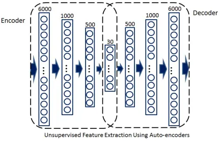
2. Deep Autoencoders

Autoencoder is another application of deep neural networks, which tries to predict

inputs. In this model, after the network is trained, features can be extracted from

the middle layers which have lower number of nodes. Autoencoders are

unsuper-vised learning algorithms used for dimensionality reduction. This model is used for

feature extraction which helps to solve overfitting in the classification problems. In

unsupervised learning labels are not used during training, thus, for training an

au-toencoder, labelled set of data cannot be used. The idea here is to let a neural

network predict its input, and be trained. Then, use the weight of this trained

(25)

some random weights while in training a network using auto encoders, the weights

of trained network can be applied for initialization. It also helps to decrease the

overfitting problem in the classification tasks.

For example, to train a deep neural network with 6 layers, an unsupervised

ap-proach is used to train the network to predict the input. Then the obtained weights

are applied for initialization, and start to train the network again. However, this time

labelled set of data is used in a supervised manner to classify data using features

extracted by Autoencoders. Another type of autoencoders is Denoising

Autoen-coders in which noise is added to the input, and that helps to reduce overfitting.

Auto encoders are considered as one of the deepest neural networks with published

results, ranging between 7 and 11 layers [26].

In the example shown in figure 2.3, the weights can be extracted from the centre

Figure 2.3: Auto Encoder that projects the input to output.

(26)

• Classification and Regression

Deep neural networks can be employed for classification and regression problems. In this

model, besides of using several hidden layers, regularization and drop out are applied as

well. In this model, deep learning is used for classification and regression as a way to find

a non-linear boundary in the data space. In an online article by Rickert [3], an example

is presented on using a data set that is distributed in the shape of a spiral (see figure 2.4),

and compares deep learning with Gradient Boosting Model (GBM), Decision Random

Forest (DRF), and Generalized Linear Model (GLM). As can be seen in figure 2.4 , the

data need a nonlinear boundary. GLM failed to classify data, since it tries to find a linear

line to separate data. The other methods could classify data into two classes. However,

deep learning is able to find more accurate boundary compared to the other models.

(27)

2.2.2.1.2 Deep Learning Parameters In this section different parameters of a deep neural networks are described.

1. Number of hidden layers:

Number of hidden layers is an important parameter in all kinds of neural networks as

well as deep neural networks. Selecting the right number for this parameter is really

important and affects the results directly.

2. Number of nodes in hidden layers:

Considering a large number for this parameter helps achieving generalization. Thanks

to regularization, selecting a big number may not lead to overfitting, however, it needs

more computation time for feeding and backpropagation.

3. Regularization:

Although Deep Neural Networks are powerful models, they have a good potential for

overfitting which occurs when the network is very complicated with too many

parame-ters, leading the network to memorize data instead of learning them. Regularization is an

approach used to reduce overfitting. Two types of regularization are used for deep neural

networks:

L2:

L2= λX

i

θ2

i (2.10)

whereθis the weight of a hidden layer andλis the coefficient of regularization, which

indicates how much regularization should be added. λ is a parameter that needs to be

tuned and finding the best value is a tradeoffbetween bias and variance. The square of

weight value is penalized in a layer. This tries to shrink the weight to be zero with a

(28)

that despite a strong regulation, bias weights are optimized. L2 is also known as Gaus-sian prior, and the reason is that it is assumed that the weights of neural networks come

from a Gaussian prior. This means that the weights of a network follows a Gaussian

distribution.

L1:

L1= λX

i

|θi| (2.11)

whereθ is the weight of a hidden layer andλis the coefficient of regularization which

indicates how much regularization should be added. λ is a parameter that needs to be

tuned, and finding the best value is a tradeoffbetween bias and variance.

In L1, the sum over square value is replaced by the absolute value. Therefore, the ab-solute value of the weight would be penalized.The difference here isL1 can push some weight to be exactly zero. Therefore, by using this regularization, network learns which

neurons should be connected to each other. When the connection between neurons are

removed, the network would be less complex and therefore less flexible. This property

results in preventing overfitting in the training data. In addition, L1 is used for input layer, because the weights can be set to zero inL1, it can do filtering for inputs. Some-times some variables in the input are not useful, andL1 regularization can act as a feature selection to remove those useless variables.

Two different parameters as coefficients are needed for L1 andL2 regularization. One reason of applying different approaches for input and output layers is that these layers

might be sparse. In the input layer, some variables are zero most of the time, and in the

output layer some neurons may correspond to a class or an event that happens rarely.

4. Dropout:

(29)

exam-ple, in random forests, combining different trees that are weak classifiers helps to make

a strong model. Similar method can be used for neural networks and train several of

them, and make a stronger model. However, for combination of neural networks some

problems may occur. Training neural networks is computationally expensive, thus, these

kinds of combination models cost a lot. In addition, different structures have to be

de-fined for each network, and tune them separately. It is difficult to tune a single neural

network, therefore tuning several of them is a demanding task. Furthermore, similar to

random forests, different training subsets are required for each model. However, in deep

neural networks, each sub-model is a neural network which needs many training data.

Thus, the training data is reduced in a model that needs huge amount of training data.

Drop out is a method which allows us to benefit from combination of different neural

networks without facing these problems. Considering a deep neural network with 10

layers, each layer is a neural network and needs to be combined with other layers which

are independent neural networks as well. Similar to random forests, they can be made

by naive predictors by disabling some nodes in each layer.

Because there is a complicated relationship between input and output, a deep neural

net-work can be overfitted easily. Dropout is introduced to solve overfitting problem. While

L1 and L2 focus on input and output layers, dropout is designed for all layers includ-ing hidden, input, and output layers. The idea is simple, and some units are required to

be selected from a certain layer and then be removed from the network. By removing

nodes form the layer, that node is disconnected from previous and next layers (see figure

2.5). In order to do this, a probability need to be assigned to each node that determines

whether it should be removed from the network or not. For example 0.5 for a certain

layer means that each unit has 50% chance to be removed from the network. Therefore,

in each layer a probability number is required to be found that determines the chance of

removing each unit (neuron) from the network. A network with 5 layers needs 5 numbers

(30)

it, roughly half of neurons from the corresponding layers are expected to be disabled.

This number can be found by cross validation and other methods used for tuning [4].

For training a network in which some neurons are disabled, stochastic gradient descent

is used similar to a standard neural network. It can be considered that after dropout, a

thinned network can be shaped, and forward and backpropagation can be applied on this

new thinned network. A special activation function is designed for the dropout that will

be discussed in the next section.

Figure 2.5: Neural net before and after dropout [4].

5. Activation function:

The typical form of output in one layer is

a= s(w0x+b) (2.12)

(31)

as activation function is very common in the classification networks. However, diff

er-ent non-linear functions also can be used for deep neural networks including hard tanh,

rectifier, and Maxout. Each of them has different properties, and here two of them are

described briefly.

• Maxout

This function is designed for dropout. The idea is to take the maximum of inputs

for each neuron in hidden layers:

Max(w0x+b) (2.13)

This idea does not work for all types of neural networks, and it works only for

feedforward neural networks (e.g. multi-layer perceptron and CNN).

• T anh

tanh(x)= sinh(x)

cosh(x) =

ex₋_e−x

ex+_e−x (2.14)

T anhmaps output between -1 and 1. Due to the fact thatT anhoutput is symmetric at 0 (is between 1 and -1), the training is better for a network with many layers. It

is worth mentioning that if these types of functions are combined, any non-linear

function can be created.

6. Learning rate:

This is one of the important parameters in deep learning. Finding a good value for this

parameter is crucial when Stochastic Gradient Descent (SGD) is being used. In SGD

each data sample is used separately during the training, while in gradient descent all

training data is used in each iteration. For example, in a problem with 100 training data,

(32)

data are given to the network once, it is called an epoch. Because a single data is used

in SGD, the update is much more variant. Therefore, a small learning rate like 0.01 is

required in SGD which works on standard multi-layer neural networks, to reduce

fluc-tuation. However, definitely finding a good value for it can improve the result. Several

techniques have been developed for a flexible learning rate to change the rate during the

training. Schedule rate can be used as a technique in which learning rate changes during

the training. A very simple schedule is to set learning rate 0.05 at the beginning, then

change it to 0.01 when the error become less than a fixed threshold, or decreasing the

rate after n iteration. Another common schedule can be acheived using equation (2.15).

learning rate= i

b+t (2.15)

wheretis the iteration number,iis initial learning, andbis the number of iterations that the algorithm needs to converge.

7. Number of training iterations:

This one is also considered as an important parameter. It should be large enough to let

the algorithm to coverage. Although, maximum number of iterations is not a tuning

parameter in a simple neural network, it is important for a deep one. In a deep neural

network, this parameter can be used as a technique to prevent overfitting. This technique

is called early stopping, and the idea is to stop training before that network converge

on the training set. Early stopping, helps to prevent overfitting problem in deep neural

networks. In this technique, validation is used to calculate the error during the training.

As long as the validation error is decreasing sharply, it can be continued. Therefore, it

shows how much iteration is enough by looking at validation error instead of training

(33)

2.2.2.1.3 Tuning Parameters Deep learning has many parameters for tuning, and several methods are used for this purpose. A validation set can be helpful to determine which

pa-rameters can lead to a better performance. Although, for this complex model, there is not a

direct relation between validation error and test error, using a validation set is the best option.

Therefore, considering a validation set is used, the following methods are available for tuning

hyper-parameters.

• Coordinate Descent and Multi-Resolution Search

This is a manual search for tuning different models, and this can be done in two ways:

First is to fix parameters, and adjust them one by one. The second approach is to try to

change all parameters at the same time. The idea of multi-resolution is to start with a big

range of number, then limit the range. For example, 100, 50, 10, 1 can be tried out and

select the best ones, then limit the range.

• Automated and Semi-automated Grid Search

The idea of grid search is to try all combinations of parameters. Using parallelization and

clustering, best possible parameters can be found. However, it is usually good for less

than 4 parameters. Humans have shown a good performance in tuning the parameters,

therefore human can help grid search to be semi-automated. The idea of semi-automated

grid search is to use multi-resolution search to guide grid search. Thus, a reasonable

range can be found by manual search, then the grid search can be performed on founded

ranges.

• Random Sampling of Hyper-Parameters

The idea of random search is to select a range for each parameter and select a number

randomly for each parameter. In many partial applications, if there are some good values

for Hyper-Parameters, random search is likely to exploit it [27]. Thus, random search

can find them without paying an exponential price (grid search). The big advantage of

(34)

servers can be used to find the best parameters.

Random search can be Semi-automated by guidance of human. In this way the random

range can be changed after running a few experiments according to the best result.

• Other methods

Some optimization algorithms are introduced that work better than random search. For

example, Bergstra et al. [28] claimed that their algorithm is better than random search,

however it works only for a special type of deep neural networks, deep belief networks.

2.3 Detection

Object detection is the main part of object tracking phase which plays an important role in the

final results and directly affects the performance of tracking.

• Point Detectors:

In point detection methods, interest points with different properties, like corners and

edges, are detected in an image instead of a whole image. Then this detected interest

points can be used for further image processing tasks. Interest points in a blob have the

same values in terms of color and brightness, and are different from their neighbor pixels.

This method is more useful in image matching applications [29]. Moravecs Detector and

Harris Detector are some examples of this type of detectors.

• Segmentation:

Segmentation methods are used in the image processing applications in order to locate

objects of interest in an image, and represent their boundaries. In this method, objects are

segmented based on their similarity in the characteristics like color, texture, and pixels

(35)

segmentation.

• Background Modelling:

It is a technique in image processing field which is based on extracting objects of

inter-ests from the background. This is used in case that the locations of objects are required

for further processing. In this method, a reference or background model is reqired in

order to extract the subtraction of current frame with it. This method is used for

detect-ing movdetect-ing objects in videos captured with static cameras and it is not applicable to the

videos recorded by moving cameras, hence, it cannot be used in the real environment

problems [31].

• Supervised Learning:

Different machine learning algorithms like SVM, Neural Networks, and adaptive

Boost-ing can be used in detection problems.

• Deep Models: Many successful results have been achieved in pedestrian detection using

Deep Learning methods. This success owes deep learnings ability in extracting proper

features from raw images without any pre-processing. There have been many

publica-tions using deep learning for object/pedestrian detection in recent years. For instance,

the JointDeep model [32] designed a Convolutional Neural Network with a hidden layer

in which jointly learns feature extraction, part deformation handling, occlusion handling,

and classification. In ConvNet [33], an unsupervised pre-trained CNN is used for

pedes-trian detection. In another work, Quyang [34] introduced a method for occlusion

han-dling in pedestrian detection considering visibility of body parts at multiple layers. In

the work presented by Tian et al. [35], TA-CNN jointly learns features from multiple

(36)

2.4 Object Tracking Algorithms

Object tracking is a crucial task in computer vision applications like car navigation,

surveil-lance, etc, containing two major steps of detecting the moving objects in each frame in a

separated detection phase, and tracking them in another step. Object tracking, usually, starts

by detecting the objects of interests in each frame in a separate phase, and suggest a big set

of detected targets, then finding the correspondence objects across frames. The task of joining

corresponding detected targets to create tracks is called data association.

2.4.1 Target Representation and Localization

It is a bottom-up algorithm to track complicated objects with complex interactions with other

objects like occlusion.

• Point Tracking

Tracking can be accomplished by considering detected objects which are defined by

points in sequence of frames. In this model the connection of the points are defined

based on the previous position and motion of the object (Figure 2.6, a).

1. Kalman Filter: (This is an equation to estimate the process status in past, present,

and future.) This is an Optimal Recursive Bayesian filter which uses a series of

observed measurements, containing statistical noise, and presents estimation of

un-known status. It is a two-stage filter in which in each iteration performs a prediction

for the current location of the moving object based on its previous location.

2. Particle Filter: (This a recursive Bayesian estimator which calculates the posterior

(37)

3. Multiple Hypothesis Tracking: In this method, all possible tracks are calculated at

first, then tracks with low probabilities are excluded using different filtering

meth-ods. This approach is really time consuming, and requires a large amount of

mem-ory.

2.4.2 Filtering and Data Association

It is a top-down algorithm for object tracking using different tools, usually with low

com-putational complexity.

• Kernel Tracking

This model of tracking corresponds to the shape and appearance of the objects in which

the kernel can be a rectangle or ellipse. The object motions in a sequence of frames

are computed to track the desired object. Motion usually refers to transformation forms

namely translation, rotation, and affine (Figure 2.6, b).

1. Simple Template Matching

2. Mean-Shift Method

3. Support Vector Machine

• Silhouette Tracking

This model can be considered as a segmentation method which tracks the objects by

es-timating the region of the objects in the frames. It is used when shapes of objects are

complex and it is not possible to describe them by simple geometric shapes. The most

important advantage of using silhouette tracking models is the ability of this model to

(38)

1. Contour Matching

These approaches estimates an initial contour of the object in its new region in the

current frame. It needs that object in the current frame have a partial overlap with

the object in the previous frame.

2. Shape Matching

These approaches search the current frame to find the object silhouette. The search

is based on the similarity of the object in the current frame with the generated model

using the hypothesized object silhouette on the previous frame.

Figure 2.6: Target Presentation Samples.

One of the methods which have good performance in multi-object tracking, is tracking

ob-jects frame-by-frame, or consider a short period of time in the sequences [36, 37]. However, to

achieve better results in case of long-term occlusions, and decrease the ratio of false positives,

and miss detections, a longer period of time can be considered in the frame sequences. It means

that more frames can be processed to solve the multi-object tracking, instead of simply looking

at one frame at a time. There are also many other works in which more global information is

used [38, 39, 40]. However, their searching spaces increase in size by increasing the number of

frames. Therefore, there should be a pruning strategy to limit the search space. Besides, they

consider all the detected objects are true positives, which it is not always the case.

(39)

frames with bounding boxes (generated by pedestrian detection algorithm). However, in their

implementation which the proposed method is compared with, they have used a part-based

HOG pedestrian detector [41] for the detection phase. Then, they applied Hungarian

Bipar-tite Graph Matching [42],to create the tracklets by finding the shortest path based on different

measures such as predicted position similarity and last position similarity measures.

The main problem of this method is that although it is locally optimal, it may not be globally

optimal due to the fact that greedy algorithms are not guaranteed to achieve the global optima.

In order to find a solution which is globally optimum, Linear Programming (LP) [43] is used

to produce a finite set of objects from the potential objects in the frames (Figure 2.7).

Figure 2.7: Linear Programming method for multi-object tracking [5] The image shows the

xandy coordinates of bounding boxes of two moving objects. The global optimum is found using ILP although objects have overlaps in some occasions.

Although LP is optimal, it has some limitations such as modelling occlusions.

• Integer Linear Programming(ILP)

ILP [43] is based on Multiple Shortest Path model in which edges are connected to the paths

which is an approach to seek for optimization of all trajectories in all frame sequences. First

step is to generate fragments of tracks, namely tracklets, produced by grouping of detected

(40)

In fact it is an approach for finding global optimum and solving the data association problem.

First, a network graph is build using the outputs of simple object detectors. Nodes in these

graphs are connected to the future and past observations.

ILP tracking formulation used by Pirsiavashi et al. [6] can model occlusion, and is globally

optimum.

By representing ILP in a flow network, the shortest path can be found using dynamic

program-ming (figure 2.8).

Figure 2.8: Representing ILP in a flow network where the shortest path is used to find the best possible track for each pedestrian.

(41)

Methodology

3.1 Detection

Convolutional Neural Networks have performed well on many vision tasks due to the fact that

it is inspired by human vision system. Due to advances in General-Purpose Graphics

Process-ing Units (GPGPU) in recent years as well as the availability of large labelled datasets like

Caltech[44] and ImageNet[45], training of large CNN have been increasingly feasible.

The main characteristics of CNN are Convolutional and Pooling layers. The former can extract

features learned by the network, and the latter allows local transitional invariances in vision

tasks. It has been shown that in case of a complicated vision task like image classification

and object detection, using features learned by CNN leads to better performance compared to

hand-crafted features [2, 46].

To train large CNN using a large dataset is crucial to decrease the chance of overfitting due to

the importance of compatibility of the model structure and data shape.

In order to be able to benefit from convolutional neural networks in case of having small dataset,

using a pre-trained CNN avoids the problem of overfitting. In the discussed problem in this

thesis, only 1000 images containing pedestrians exist to be tracked. Therefore, it was decided

to use a Deep convolutional network, DeepPed [10], pre-trained on a large dataset, Caltech

(42)

Pedestrian [47], which is a large-scale and widely accepted dataset. Caltech Pedestrian Dataset

is about 10 hours of video taken in an urban location by a vehicle driving through the

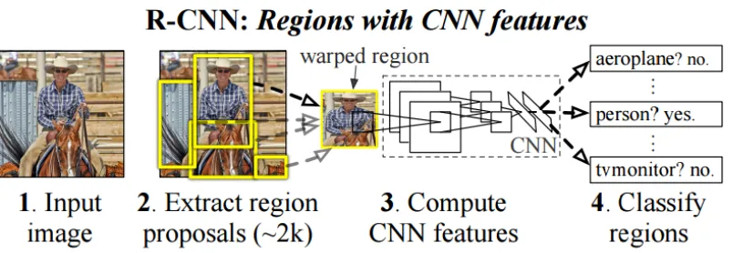
environ-ment. DeepPed is a pedestrian detector algorithm which is based on R-CNN [46]. The main

characteristic of this algorithm is combining rich features achieved by a convolutional neural

network with region candidates that are likely to be pedestrians. The structure of R-CNN can

be seen in the figure 3.1.

Figure 3.1: R-CNN structure 3.1

In DeepPed, a detection algorithm called Locally Decorralated Channel Features (LDCF)

[48], is used which proposes a large set of regions with a confidence value for each region

indicating increase the probability of each region to be a pedestrian. The output of DeepPed

is a set of bounding box positions as well as their corresponding frame numbers which can be

used for tracking.

3.2 Visual Tracking

The process of locating objects in a video is considered as visual tracking. The object may be

(43)

In many methods of object tracking, objects are initialized manually, or even number of objects

in the video is defined. However, in the presented method, there is no need for any initialization,

and algorithm can figure it out itself. The tracking step in this work is mostly based on the

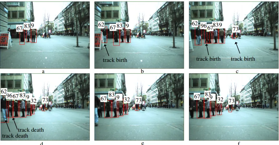
method presented by Pirsiavashi[6]. In their method, the goal is to (a) find out the number of

tracks appear in the sequences and (b) defining the start and end of tracks. Figure 3.2 shows

some samples of start and end points in the tracks.

Figure 3.2: This figure shows tracked pedestrians with specified label numbers as well as births and deaths of tracks of individual pedestrians.

In the Pirsiavash work [6], a set of frames in containing bounding boxes detected by a

part-based HOG pedestrian detector [41] is assumed as the input. The authors presented a globally

optimal multi-object tracking algorithm using a low-level tracker and a graph-based algorithm.

Their work is based on the min-cost flow algorithm presented in an analysis of an integer linear

programming (ILP) formulation in [43], popular in recent literature. In linear programming,

tracking problem is modelled as a multiple-path searching problem and optimizes the detected

tracks in terms of finding a consistent track for all the objects, and the locations that objects are

(44)

tracks number, and the birth and death state of the tracks. They presented a method to find the

global solution using a greedy algorithm in which tracks are computed by finding the shortest

path in a flow network. I have decided to choose this method, since they have used fast and

simple algorithms which make it suitable for my goal.

3.3 Post Stage Processing

In order to improve the performance of the tracking results, a post stage processing step after

all detection, and tracking steps is proposed. At this level, results consist of both completed

tracks as well as broken tracks. The goal in a tracking algorithm is to have smooth tracks

containing bounding boxes with the same IDs. Broken tracks are an important issue at this stage

leading to a reduction in tracking performance. Broken tracks are short tracks with different

IDs containing a few number of bounding boxes. These broken tracks can be joined to the best

matches among the other tracks to have smoother tracks and decrease the number of broken

tracks. For this purpose, in a set of temporal sequence of frames as the pedestrians move, ends

of each track are considered as well as the beginning of all the new tracks started in the next

frame. Then, Euclidean distance is used to find the closest detected track starting in the next

frame to the ended track in the current frame. In order to make it more precise, a threshold was

defined to consider only those bounding boxes which are in the specific threshold area. It is

worth mentioning that same threshold values are used in the second experiment on the video

recorded at Western..

This approach reduces the number of broken tracks as long as the detection part has a high

accuracy in pedestrian detection. However in my case, DeepPed misses some pedestrians in

one, two or more than two frames, and this causes broken tracks due to the fact that I am using

a different dataset rather than the one that DeepPed was trained with. Simply using Euclidian

distance in not enough to distinguish between bounding boxes and find the one which is the

(45)

the algorithm to attach tracks to their continuation, and it simply finds the closest bounding

box. By only using Euclidian distance for measurement, information about other factors like

appearance of targets, motion direction of targets, and size of targets cannot be achieved.

Figure 3.3: Limitation of simply using euclidian distance to join the broken tracks.

Figure 3.3 shows a case where only using Euclidian distance leads to a wrong result. The

purple bounding box shows the right location of the person in the red bounding box in the

next frame. However, as can be seen in figure 3.3, the blue bounding box is closer to the

red bounding box. Therefore, the blue bounding box mistakenly will be considered as the

(46)

the second-order features from each bounding box is proposed to define whether the bounding

boxes in each frame are the continuation of the track in the previous frame. In other words,

contrast of the current bounding box is computed using equation 3.1 and compared with the

contrast value of other candidates.

Contrast =X

I1,I2

|I1−I2|2logp(I1,I2) (3.1)

This helps to compare pedestrians in each track and find the best match based on their

ap-pearance. Then, a threshold is defined for this part to improve the accuracy. The value of the

threshold is defined by trial and error. However, it is worth mentioning that the same values

of the thresholds are used in both experiments, on ETHZ and the dataset recorded by myself.

It shows that these values are robust enough that they can be used on new datasets containing

pedestrians.

However, using only these features is not accurate enough and leads to incorrect detection of

the desired bounding box, in cases that a bounding box is found in the desired threshold range

of second order features while it is totally far from the target. To solve this issue, a mixture of

second order features and Euclidean distance from the centre of each bounding box was used.

The flowchart of the proposed Post Stage Processing is shown in figure 3.4. Moreover, finally,

the number of false positive tracks are narrowed down by considering a threshold to exclude

those tracks containing less than five tracked bounding boxes.

3.4 Algorithm and Software Development Steps

Software environment consisted of MATLAB 2013a running on Ubuntu 14.04 on a desktop

which features a Core-i7 3.7 GHz Intel processor, 32 GB RAM , and Geforce GTX 760 GPU.

For DeepPed algorithm installation, Caffe, which is a Deep Learning framework, was installed.

(47)

(BVLC). At the first step, Caffe needs a number of prerequisites which should be installed.

These include CUDA v7+ (required for GPU mode), BLAS v3.6.0, Boost v1.55, OpenCV

v3.0, and IO libraries: lmdb, leveldb. Then Caffe v0.999 package was installed. Since DeepPed

is based on R-CNN, the R-CNN package was installed as well. Then, DeepPed package was

installed to do the detection phase. After installing DeepPed, MATLAB implementation of the

tracking algorithm v1.0 was installed. Then DeepPed was fed with all the frame sequences in

the ETHZ dataset in order to detect pedestrians. The output of DeepPed was a set of bounding

box positions as well as their corresponding frame numbers which were used for tracking.

Then, tracking algorithm was performed on the new data and the tracking results were recorded

as a video stream at the end. After all these steps, a Post Stage Processing was implemented

to improve the accuracy (Matlab function PostStageFunction is used to perform the proposed

Post Stage Processing). It started by finding the end of all the tracks in all of the frames using

function TracksSmoother3framesFunc. Then the next frame was checked for the newly started

tracks since there was a probability that one of these newly started tracks to be the continuance

of the lost track. Therefore, they were compared to the lost track in order to find the best match.

Function trackFrame1 finds the best matched tarck in the next frame. To find the best possible

match, first, candidates which were close to the lost tracks were considered using Euclidian

distance. Then, among these candidates, the most similar pedestrian to the lost pedestrian in the

track was selected based on the similarity of their contrast attribute. In the case of finding the

best match, tracks were joined by assigning the same labels. If the best match was not found,

two next frame were checked to find the best possible candidate using function trackFrame2.

And again, if none of the newly started tracks in the two next frame were matched with the lost

track, based on the same Euclidian Distance and contrast conditions, the three next frame were

checked for the tracks started in this frame. Function trackFrame3 finds the best possible track

in the three next frame. This process is illustrated in the flowchart 3.4. All the code for the post

(48)

3.5 Dataset

Many datasets have been presented for multi-object tracking using stationary cameras, namely

CAVIAR project and PETS2009 datasets [49, 50]. Doing experiments on a dataset with moving

cameras is more challenging compared to the stationary ones. In this experiments, ETHZ

dataset [51] is used containing both left and right view of a crowded sidewalk which is recorded

by cameras attached to a moving stroller. Only the left view of this dataset is used in this work.

It consists of four videos each containing about 1000 frames, exported from the video at 14

frames per second. Figure 3.5 shows a sample frame in ETHZ dataset. All the bounding boxes

in the dataset are annotated, however, there are no annotations for the track labels. In order to

be able to evaluate results of the presented method with the others results, track ID annotations

which are defined manually and presented by Milan [52] are used.

I also created a dataset to see the performance of my method on a different input video

as well. In order to create this dataset, a camera is fixed in a hallway and recorded about 4

minutes of video, captured from students walking in the hallway. I asked about six students to

help with recording this video. It was important to have multiple individuals to be visible in the

frames since the suggested algorithm in this thesis works best in tracking multiple pedestrians

as shown in figure 3.6. In addition, in this dataset, it is tried to include occlusion as well as

distance in this dataset. By distance, it means that this video is recorded in a long hallway to

evaluate the proposed method in facing pedestrians which are very small due to their distance

(49)

3.6 Evaluation

Many methods have been presented in recent years for multiple object tracking, however, there

is no specific agreement on the way to evaluate and compare all these methods, and lack of

common metrics for evaluation of multiple object tracking algorithms makes it difficult to

compare results with the existing algorithms easily. In addition, literature on such evaluation

methods is rather sparse. Due to these issues, several methods for multiple object tracking

present their results without a quantitative evaluation [53, 54, 55].

Method presented in this work is evaluated by CLEAR-metrics presented by Bernardin et al.

[56].

• Multi-Object Tracking Precision (MOTP)

MOTP is the total error which simply computes the average of distancedi

t between true

objects tracked in the ground truthGi

t and hypothesized tracked objects D i

t, andct, the

number of track matches made in frame t. It shows the precision of the tracking algorithm

in estimating objects positions without considering the other factors including keeping

consistent trajectories (3.2).

MOT P=

P

i,tdti

P

tct

,where dti =

Gi T T Di T Gi T S Di T (3.2)

• Multi-Object Tracking Accuracy (MOTA)

This method evaluates the multiple object tracking algorithms in terms of accuracy, in

which false positives f pt, missed objectsmt, and ID switches are taken to the account.

MOT A =1− P

(f pt+mt+mmet)

P

gt

(3.3)

This formulation is derived from three miss rate error, false positive ratio, and

(50)

m=

P

tmt

P

tgt

(3.4)

f p=

P

t f pt

P

tgt

(3.5)

mme=

P

tmmet

P

tgt

(3.6)

In order to evaluate the presented method, results are compared to the results achieved by

the method presented by Pirsiavash [6]. It is tried to consider similar conditions, like using

same dataset as well as the same ground truth, for both methods to have a trustable evaluation

(51)

(52)

(53)

Figure 3.6: Sample image from my dataset, showing multiple pedestrians.

(54)

Results

The proposed method is evaluated on the ETHZ as well as a video recorded by myself.

• Detection

As described in section 3.1, the pre-trained deep neural network, DeepPed [10] is used

for the detection step. Comparing the suggested detection phase results with the

annota-tions in the original video sequence as well as detection method used in Pirsiavash et al.

method [6] shows that DeepPed in many cases is more precise in detecting pedestrians,

even the pedestrians that are not annotated in the in the original video sequence.

Fol-lowing figures visually show these differences between results of the proposed algorithm

with both the original video sequence and the method used in Pirsiavash et al method

[6].

• Tracking

As can be seen in the results in table 4.1, two factors, True Positive Ratio (TPR) as well as

False Negative Ratio (FNR) have better results compared to the Pirsiavash et al. method

[6]. The Total True Positive Ratio(TPR), False Positive Ratio (FPR), False Negative

Ratio (FNR), and True Negative Ratio (TNR) are computed based on the equations 4.1,

4.2, 4.3, and 4.4 respectively.

(55)

Figure 4.1: (a) represents a specific frame in the tracking results of the proposed method in this thesis. (b) is the same frame which shows the result of tracking method presented by Pirsiavash et al. [6], and (c) shows bounding boxes annotated in the same frame of the original video sequence.

Table 4.1: This table shows the actual True Positive (TP), False Positive (FP), False Nega-tive (FN), and True NegaNega-tive (TN) values of the final tracking results in both Pirsiavash et al. method [6], as well as the proposed method.

TP FP FN TN

Presented Method 4982 1285 2509 6361 Pirsiavash et al. [6] 4870 276 2653 7370

T PR = T P

(T P+FN) (4.1)

FPR= FP

(FP+T N) (4.2)

FNR= FN

(FN+T P) (4.3)

T NR= T N

(FP+T N) (4.4)

Proposed method is evaluated using CLassification of Events, Activities and Relationships

(CLEAR) metrics [56], since these metrics are very presice in multi-target tracking evaluation,