ISSN 2286-4822 www.euacademic.org
Impact Factor: 0.485 (GIF) DRJI Value: 5.9 (B+)
Application of Spatial Calculating Analysis Model
for Land Use Conversion in Colombo Urban Fringe
W. H. T. GUNAWARDHANA
K.G.P.K. WEERAKOON Department of Estate Management and Valuation University of Sri Jayewardenepura Sri Lanka
Abstract:
Key words: Land conversion, Urban land use, Urban fringe, Spatial Calculating Model
1. Introduction
The history of urban growth and urbanization reveals that urban areas belong to the most dynamic land cover types on earth. It forces to socio and economic development (Thapa & Murayama 2011) that leads to the land use and land cover change in the urban-rural fringe. Regardless of the regional economic importance, urban growth, particularly the expansion of urban growth towards the periphery of urban areas has an impact on the ecosystem (Hu et al. 2007; Thapa & Murayama 2010). It is evident that such trend of urban growth has an impact on natural resources and on land cover dynamics at large. (Thapa & Murayama 2010)
According to that land conversion in urban fringe area is a continuous process and it is of timely importance to analyze such a land conversion prior to making a decision to mitigate the above problems. Manual calculation of existing changes does not provide an exact picture of those changes. To obtain a clear picture it is needed to be analyzed in a scientific way. Over the last decade, GIS has grown dramatically and its sophisticated analysis tools provide a better insight for different kind of spatial analysis (Chang & Masser 2003). Most researches applied GIS for identifying land use changes. In 2008, Xinchang et al. developed a spatial calculation model for identifying land use changes in the urban fringe area.
environmentally sensitive marshy lands have been filled by private developers. In some areas, nearly 50% of agricultural lands have been converted into urban uses (Ariyawansa 2008). Further, rapid increasing land prices and uncontrolled land markets stimulate poor land owners to sell their lands to private developers which is relatively advantageous with increasing land price than their existing land uses.
These rapid land use changes create some positive as well as negative effects to the society and environment. Different social, economical, political and environmental factors are causes for that. However, urban fringe areas are converted into urban uses at an alarming rate. This process threatens the sustainable development and its impact is unable to be measured. Hence, the land use changing pattern, intensity of changes and its consequence cannot be adequately measured due to lack of scientific methodology. So, it is very important to have a scientific, systematic and reliable technique to evaluate land conversion pattern of urban fringe area for decision making (Chang & Masser 2003). This study aims to develop some methodological approach for that.
2. Objectives of the Study
The General objective of this study is to develop a model to analyze and calculate land use changes using a scientific methodology during specific periods. For fulfilling this main objective, following specific objectives were developed.
To analyze the land use changes during the 13 years period.
3. Review of Literature
3.1 Land use
Land use is a business between man and natural environment. Hence, Briassoulis (2008) stated that the land use change is the result of a complex web of interactions between bio-physical and socio-economic forces over space and time. The magnitude of land use change varies with the time period being examined as well as with the geographical area. Moreover, assessments of these changes depend on the source, the definitions of land use types, the spatial groupings and the data sets used (XinChang et al. 2008). However land uses pattern changes are different from area to area. Pattern of rural areas’ land use changes totally different from urban land use change. Because land use types are different from area to area (Majeed 1996). For example while most rural areas land conversions are from forest lands to agriculture lands, urban agricultural lands being converted to residential, industrial uses etc. In any situation land use changes are very difficult to critically identify, because of its complex and dynamic nature (XinChang et al. 2008).
Growth of urban areas depends on both economic and non-economic factors (Harvey 2004). Economic factors are the nature of existing economic opportunities in a nation determined by the size and character of the future urban population, level of income, consumption need and land use etc. Non-economic factors are significantly interrelated with economic factors and vice versa; those are population changes, advanced in technology and policy changes etc. (Harvey 2004). Ultimately those two factors cause urban growth and simultaneously results in changing the existing land use pattern.
Deriving those changes is a complex process due to its complexity. Modeling of land use changes (as a function of its biophysical and socio-economic driving forces) provides insights into the land use changes and its effects (Weerakoon et al. 2008).
3.2 Land use change Models
Models are a formal representation of reality and also sometimes it represents theory of a system of interest (Briassoulis 2008). The representation of reality is expressed through the use of symbols and formulas (XinChang et al. 2008). Models of land use change can play an instrumental role in impact assessment of past or future activities in the environmental and/or the socio-economic spheres. Models of biophysical and/or human processes operate in a temporal context, a spatial context or both. When models incorporate human processes, the human decision making dimension becomes important. In reviewing and comparing land use change models along these dimensions, two distinct and important attributes must be considered: model scale and model complexity (Lambin 1994).
models distinguished like spatial interaction models (Spatially explicit land use models), statistical and econometric models, optimization models and integrated models. All these models can be identified as numerical models or conceptual models.
3.3 Numerical model for Land use changes.
Numerical models are one of the best methods that can be used to calculate land use changes. According to Bruce and Maurice (1993), Land-use changes during a certain period can be shown by calculating the average changing ratio of land-use model in the researched region. The principle of this theory is based on general mathematical calculation for finding some changes over time. For an example, calculation of Population growth rate, Death rate etc.
The mathematical expression for measuring land use change can be formulated as follows;
CRi = (TA (i, t2) - TA (i, t1)/TA (i, t1)/ (t2-t1)*100%
Where, CR is changing Rate, TA is Total Area, i is Land use type and t is time (year).
For instance when applying above expression for land use change of paddy during 1990 – 2000, it is as follows;
CRPaddy = (TA (Paddy, 2000) - TA Paddy, 1990)/TA (Paddy, 1990)/ (2000-1990)*100%
The main advantages of the calculating model are shortness and simplicity and we can use it without complicated professional analysis. It is used in both professional and non-professional reports and academic papers.
But the disadvantage is obvious as well.
1) This model ignores the fixity and distinctiveness of land-use spatial position, and cannot reflect the spatial process and interrelated attributes of changing land-use dynamic.
with spatial locations and attributes different, but acreage completely the same: On one hand, barren unused land is reclaimed far from the city; on the other hand, a field of high quality is converted into land for civil construction near the city. The two changing processes counteract each other and cannot reflect the actual condition when we analyze the dynamic changing of the region.
2) This model cannot calculate and compare the active degree of land-use changes, that is to say, it cannot distinguish the “hot” or “sensible" district, as it has no spatial characters.
3.4 Spatial Calculating Analysis Model
categories as follows:
I. Unchanged part- Same land use pattern exists during
case study period. This result in keeping the same extent of subject use as in the beginning.
II. Converted part-Some specific land use has changed
into another use by the end of case study period. That conversion of use is considered as the converted part. This results in reducing the subject use extent and increase another use or uses.
III. Increased part- The accumulated area for subject land
use pattern during the case study period. For example, Agricultural area might be increased by clearing the forest area. Then, it can be seen an increased area of agricultural land (Xinhang et al. 2008). Further study illustrated that situation in the following figure 1. As a whole, land use changes are represented by either converted part or increased part. At the same time, there is a close relationship between these two. Because converted part results in increasing another use and vice versa.
Xinchang et al. (2008) state results obtained from spatial calculation model are used to find out why the situation can take place by combining social and economic situations. The result indicates the calculating analysis model of spatial information and can derive a more accurate procedure of spatial transference and increase all kinds of land from a microcosmic angle. By this model and technology it is easy to conduct the research of land use spatio-temporal structure evolution more systematically and more deeply, and can obtain a satisfactory result. And also in the case of application of these models GIS can be used as a tool.
4. Methodology
changes in urban fringe area using GIS (Geographical Information System). On this basis GIS plays a major role to analyze existing situation compared with the past situation. Further, field survey data collection (Discussion with villagers) is used to correct doubtful areas of existing data. Hence, this study consists of the following areas.
Study area consists of several GN divisions. And also land use changes differ from each GN division. Hence all GN divisions are selected to study. Therefore, Selected Sample is the total area of Homagama Pradeshiya Sabha (HPS).
General objective of the research is to calculate the land use changing rates for each use during 1981 to 2004. According to the literature review, basically it requires collecting secondary data and in case of the need, primary data for verifying the secondary data. Therefore, based on availability of secondary data, it has selected land use data in 1981 and 2004, where 1981 data has to be moderated so that it is compatible with 2004 data structure. Because in 1981 HPS area was different from 2004 PS limits. Study is mainly based on field survey for identifying land use changes and boundary differences.
Though both data sets are past in 1981 and 2004, those are different in extent and boundaries. And also 2004 data are in digital format and in 1981 data are abstracted from a paper map. Therefore, 1981 data has to be converted into digital format using GIS and doubtful areas need to be checked. Because, some Paddy land which appeared in 1981 has changed into Rubber land. Generally, Paddy lands are not used for Rubber cultivation. Likewise, general overview of accuracy of the data should be rechecked and updated by using a field survey. 1:2000 land use map prepared by the survey department of Sri Lanka was use as a base map for analysis.
4.1 Development of Spatial Calculation Model
Analysis model is a modification of numerical model for measuring the land use changes. Hence, disadvantages of using a numerical model can be minimized. Because it concerns not only the state of beginning and end of a particular use but also the variation of such uses throughout the study period.
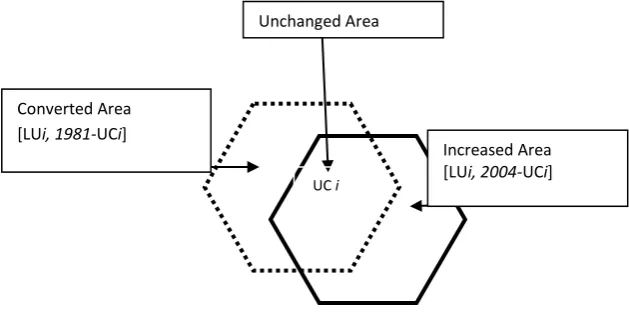
The spatial calculating analysis model is based on GIS overlay. It compartmentalizes the case study area land (Homagama PS Area) into three spatial parts: like unchanged, converted and increased areas. Following figure 4.1 illustrates the concepts of Converted, Unchanged and Increased areas, where LUi means the selected land use category. For example Agriculture, Built up areas etc.
Figure 4.1 Land use classification according Spatial Calculating analysis Model
Source: Developed based on spatial calculation model, XinChang et al, (2008)
By this model it is possible to evaluate the numerical model and dynamic degree model for existing calculating changing speed of land use. Furthermore the result rise reviving the calculating analysis model of spatial information in order to predict the dynamic changing level of all sorts of land. More concretely speaking, the model is mainly to know the changing area and changing speed (increased or decreased) of different land classifications to clearly show the spatial distribution of
Unchanged Area
Increased Area [LUi, 2004-UCi] Converted Area
[LUi, 1981-UCi]
changing urban lands. The result will benefit the planning and management of land-use of HPS area in the future.
I. Unchanged part-Here, it can be seen that a particular
use remains unchanged during the case study period. This results in keeping the same extent of subject use as in the beginning. For example, unchanged Agricultural land area during 1981-2004. GIS is used as a tool to select this unchanged area. Accordingly, each similar land use categories from 1981 and 2004 are taken and overlapped to select the common area of each and it is called the unchanged area of each category during 1981 to 2004, because these common areas are constant during the study period.
II. Converted part- Some specific land use has changed
into another use by the end of the case study period (1981-2004). For example, Agricultural land in 1981 has converted intoresidential use by 2004. That conversion of use is considered as converted part area of Agriculture use. This results in reducing the subject use extent and increase another use or uses.
4.2 Calculation of dynamic land use change rate for converted area
Converted area means the area that has changed into another use during the study period. For example 977.76 ha of Coconut land has changed into another type of use by 2004. Hence, the intensity of such a change can be measured by the following formula.
CRi = (TA (i, 1981)-UCi)/TA (i, 1981)/ (2004-1981)*100%
In that model CR is converting rate per year, i is a particular land use type, UC is unchanged area of relevant land use type and TA is total area of that land use type.
III. Increased part- The accumulated area for subject land
Agricultural area might be increased by clearing the forest area. Then it can be seen an increased area of agricultural land. Similarly, increased area is accumulated or adjoined area of selected land use category into another use during the research period. For an example, some Paddy area in 1981 has been converted into Residential use by 2004. That area is called as increased area of Residential use etc.
As a whole, land use changes are represented by either converted part or increased part. At the same time, there is a close relationship between these two. Because converted part results in increasing another use and vice versa.
4.3 Calculation of dynamic land use change rate for increased area
Dynamic land use changes the rate of increased area of a particular use, which measures the intensity of increase of a particular land use type. This is also calculated using following formula and result is in a percentage.
IRi= (TA (i, 2004)-UCi)/TA (i, 1981)/ (2004-1981)*100%
Here, IRi means the increasing rate percentage of a particular land use pattern. All other variables are similar to converted rate calculation formula.
4.4 Aggregate model for land use change analysis
To get a reasonable conclusion about land use changing speed of a selected use, it is important to consider both conversion and increasing parts. Therefore, Total changing speed or aggregate land use change percentage is calculated as follows;
ARi= (TA (i, 1981)-UCi)/TA (i, 1981)/ (2004-1981)*100% + (TA (i, 2004)-UCi)/TA (i, 1981)/
(2004- 1981)*100%
5. Data Analysis
5.1Case study area
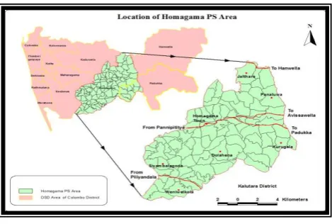
Homagama Pradeshiya Sabha (HPS) is situated in the Western Province of Sri Lanka within the Colombo district. It is located 21 Km away from the City of Colombo along the High level road. The high growth in the City of Colombo during the past decades has made an impact on Homagama to be developed as a service center. Location of residential clusters, the Industrial parks of Katuwana, Panagoda and Meegoda, Diyagama International Sports Stadium, Main interchange of Southern Highway, Nano Technology Park, Information technology park, Godagama economic development center are the main service centers attracted to the growth of this area. In the Colombo core area plan, Homagama has been categorized as a fourth order township. Further, Godagama, Habarakada, Meegoda and Polgasowita are important sub-centers in the area. Homagama is also linked and has interrelationship with the surrounding
service center of Athurugiriya, Kaduwela, Malabe,
Maharagama, Kottawa, Piliyandala, Horana, Padukka, Ingiriya and Hanwella.
Figure 1: Location of case study area
This area is predominantly an agricultural area and it consists of a low residential density of 14 persons per Ha. During the last inter censual period, population growth rate has been increased up to 2.92% per annum. This growth rate is higher when compared with the other local authorities in Colombo district.
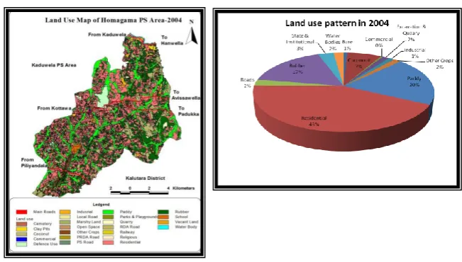
5.2 Existing Land Use Pattern
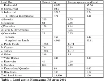
According to Homagama Development Plan, the land extent of Homagama Pradeshiya Sabha area is 13,820 ha. Out of the total land extent 48% (6572 ha.) is under residential use. Agricultural use is 36% (4949 ha.) The agricultural land use is decreasing with the growth of population. However, agricultural sector is dominant in the local economy. The existing land use pattern is shown in the following table 1 and figure 1.
Land Use Extent (Ha) Percentage as a total land
1. Residential 6,572 47.56
2. Commercial 92.5 0.67
3. Industrial 379.5 2.74
4. State & Institutional 471 3.41
a)Security 220 1.59
b)Religious 64 0.46
c)Education 158 1.14
d)Parks & Play grounds 7 0.05
e)Cemeteries 22 0.15
5.Roads 756 5.47
6. Agriculture Lands 4,949 35.81
a. Paddy Fields 1,996 14.74
b. Coconut 744 5.38
c. Rubber 1,960 14.18
d. Other 249 1.8
7.Water Bodies 344 2.49
a. Reservoirs 40 0.28
b. Marshes 304 2.19
8. Excavations/ Quarries 93 0.67
9. Bare lands 163 1.17
Total Land Extent 13,820 100
Table 1 Land use in Homagama PS Area-2007
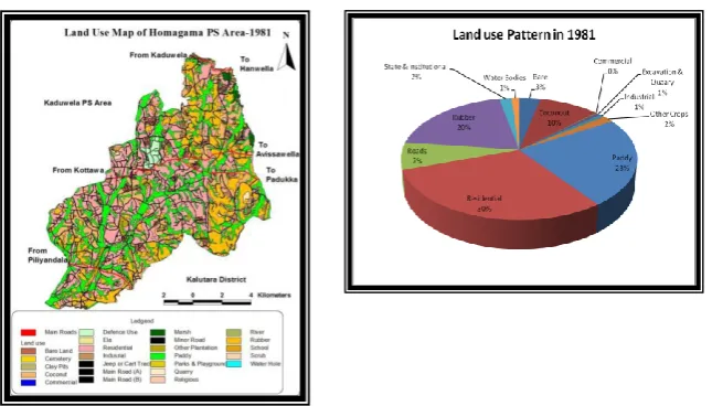
In 2007, HPS area was updated and boundaries were changed. So, 2007 land use map cannot be compared with the 1981 map. Therefore 1981 and 2004 maps were selected for application of spatial calculation model. The model illustrated the land use changes of a 13 years period. But land use categories are different in those two years; hence before applying the model it should be converted to common land use categories. According to that land use categories on two different years can be classified as follows in figure 2.
Figure 2: Landuse Map Homagama
Figure 3: Land use pattern of Homagama PS Area in 2004.
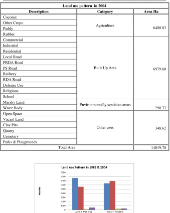
Land use pattern in1981
Description Area Ha Category Area Ha
Coconut 1345.42
Agriculture 7682.13
Other Plantation 261.54
Paddy 3287.27
Rubber 2787.90
Commercial 24.26
Built up Area 5587.63
Industrial 110.96
Residential 4185.39
Jeep or Cart Track 370.31
Main Road (A) 50.34
Main Road (B) 43.48
Minor Road 552.15
Defense Use 214.93
Religious 8.96
School 26.87
Ela 30.18
Environmentally sensitive areas 166.86
Marsh 106.74
River 27.76
Water Hole 2.18
Bare Land 470.92
Other uses 583.21
Clay Pits 16.93
Quarry 60.03
Scrub 18.05
Cemetery 15.27
Parks & Playgrounds 2.00
Land use pattern in 2004
Description Category Area Ha
Coconut
Agriculture
6400.83 Other Crops
Paddy Rubber Commercial
Built Up Area
6979.60
Industrial
Residential Local Road PRDA Road PS Road Railway RDA Road Defense Use Religious School Marshy Land
Environmentally sensitive areas
290.73 Water Body
Open Space
Other uses
348.62
Vacant Land
Clay Pits Quarry Cemetery
Parks & Playgrounds
Total Area 14019.78
Figure. 4: Changes of four major land use categories during 1981-2004
up to 45.54% of the total area by 2004. Secondly, Built up area consists of 5587.63 Ha or 39.85% of total area in 1981 and it has increased up to 49.78% by the year 2004. Hence, it is obvious that the trend is to convert agricultural land into built up areas like residential, commercial and industrial etc.
In addition to those, environmentally sensitive areas and other uses like bare land, scrubs etc are 1.19% and 4.16% respectively in 198. But by 2004 aforesaid other uses have reduced and environmentally sensitive lands have increased. Construction of new irrigation systems and declaration of irrigation reservation areas caused to increase the areas which are environmentally sensitive by 2004.
As in the above figures, it is only possible to determine the changes of each category. For example agriculture uses are being converted into built up areas etc. But it doesn’t give a clear index to determine the conversion trend accurately. As described in the literature review numerical models are not reliable and accurate. Therefore “Spatial Calculating Analysis Model” can use be used as follows;
6. Application
Data analysis is basically done by using GIS and MS Excel. Here, when analyzing data, GIS is used as an analytical tool, data processing tool and data presentation mode. Therefore, it is possible to obtain reliable data so that it can be used to prepare maps, charts etc.
6.1 Data Modification using GIS
And also in 1981 paper map doesn’t indicate the declared area for Defense use. But actually that area should appear in 1981 data too. So such modifications are done prior to data analysis.
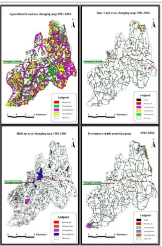
6.2 Data analyze using GIS
At first it needs to identify separate themes for each land use category from both 1981 and 2004 data sets. For instance, Agriculture uses themes in 1981 and 2004 etc. There are four different themes for each land use category so that it is able to compare one another.
Those are
Agriculture use
Built up areas
Environmentally sensitive areas
Other uses
6.3 Comparison of land use changes 1981-2004 in HPS Area
When taken the whole built up area into consideration, an important category of the land use change is residential. Other land uses in built up area are not significant.
Total Land use changing rates during 1981-2004
When considering all the above information land use changing rates for each category can be calculated using Spatial Calculation Model. Hence it is easy to identify not only the total conversion rates or intensity of land use changes but also Converting rates and increasing rates for each land use category. And also based on aggregate land use changing rates (AR), it is possible to predict the future trend of each land use changes in Hectare. Therefore, both extent and changing rate need to be considered to get a comprehensive idea of changes.
Further, this result can be analyzed according to converting rate and increasing rate. In that scenario 146Ha of agriculture land is to be converted into another use by year 2005. Accordingly, Figure 3 indicates the land use changing pattern of major four categories Agriculture, Built up Areas, Environmentally sensitive area and other uses. However land use changing pattern of main four categories (Figure 3) doesn’t give a clear idea about its use. Hence, Table 3 indicates the detailed analysis of each land use with Converting rates and increased rates and ultimately aggregate land use changing rates (AR) for each land use category. Therefore it is easy to identify and predict the most endangered Agriculture use etc. for example paddy land is more sensitive to change-66 Ha per annum. Accordingly, changing pattern of each use can be predicted using AR rates.
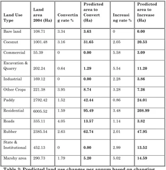
Following table suggests the predicted land use changes in the future. Therefore, it is easy to identify the highly converting uses, highly increasing uses etc. So, these results can be used to prepare plans, policies, and regulations to make comprehensive and sustainable development of Homagama PS area.
Land Use Type
Land area 2004 (Ha)
Convertin g rate %
Predicted area to Convert (Ha)
Increasi ng rate %
Predicted area to Increase (Ha)
Bare land 108.71 3.34 3.63 0 0.00
Coconut 1001.48 3.16 31.65 2.05 20.53
Commercial 55.39 0 0.00 5.58 3.09
Excavation &
Quarry 202.24 0.64 1.29 5.54 11.20
Industrial 169.12 0 0.00 2.28 3.86
Other Crops 221.38 3.95 8.74 3.28 7.26
Paddy 2792.42 1.52 42.44 0.86 24.01
Residential 6005.52 1.59 95.49 3.48 208.99
Roads 335.11 4.05 13.57 1.14 3.82
Rubber 2385.54 2.63 62.74 2.01 47.95
State &
Institutional 452.13 0 0.00 2.99 13.52
Marshy area 290.73 1.79 5.20 5.02 14.59
Table 3: Predicted land use changes per annum based on changing rates
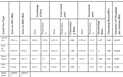
Table 4: Land use changing rates based on Spatial Calculation Analysis Model 1981-2004
According to the above table 4.3, Agriculture land use changing rate is only about 3.86% per annum. Which is the lowest changing rate compared with other uses. And also highest changing rate of the water bodies are 6.81% per annum. But the impact of these rates depends on the total area of each use. Therefore that impact on each land can be identified in “Intensity of Changing per Annum (Ha)” column in table 4.3.
L and U se T yp e Ar ea in 19 81 (H a) Ar ea in 20 04 (H a) Un cha ng e d Pa rt Conv er te d p ar t Incr ea se d p ar t Chang ing R a te (AR )% Int en si ty of C han gi n g p er An nu m (H a) A re a T ota l A re a
% Are
a T ota l A re a % Conv er ti n g R a te A re a T ota l A re a % Incr ea si n g R a te Agricul
ture 7682.12 6400.83 3630.2 25.89 4051.91 28.9 2.29 2770.59 19.76 1.57 3.86 247.07
Built up
Area 5587.63 6979.6 3123.9 22.28 2481.01 17.7 1.92 3873.05 27.77 3 4.92 343.40
Water
Bodies 166.86 290.73 98.14 0.7 68.72 0.49 1.79 192.59 1.37 5.02 6.81 19.80
Other
uses 583.26 348.62 189.77 1.35 234.65 0.87 2.93 0 0.86 1.18 4.12 14.36
L and U se T yp
e Un
cha ng ed P ar t Conv er te d p ar t Incr ea se d p ar t Chang ing R a te (AR )% Int en si ty of chan gi ng H a p .a Ar ea T ot al Ar ea % Ar ea T ot al Ar ea % Co n v ert in g R a te Ar ea T ot al Ar ea % In cre a si n g R a te
Bare 108.7 0.78 108.7 0.78 3.34 0 0 0 3.34 3.63
Coconut 367.64 2.62 977.76 6.97 3.16 633.81 4.52 2.05 5.21 52.18
Commercial 24.26 0.17 0 0 0 31.14 0.22 5.58 5.58 3.09
Excavation
& Quarry 81.07 0.58 13.95 0.1 0.64 121.18 0.86 5.54 6.18 12.50
Industrial 110.96 0.79 0 0 0 58.16 0.41 2.28 2.28 3.86
Other Crops 23.92 0.17 237.62 1.69 3.95 197.47 1.41 3.28 7.23 16.01
Paddy 2139.91 15.26 1147.36 8.18 1.52 652.51 4.65 0.86 2.38 66.46
Residential 2651.9 18.92 1533.48 10.94 1.59 3353.3 23.92 3.48 5.08 305.08
Roads 68.75 0.49 947.53 6.76 4.05 266.35 1.9 1.14 5.19 17.39
Rubber 1098.73 7.84 1689.17 12.05 2.63 1286.8 9.18 2.01 4.64 110.69
State &
Institutional 268.03 1.91 0 0 0 184.1 1.31 2.99 2.99 13.52
Marshy area 98.14 0.7 68.72 0.49 1.79 192.59 1.37 5.02 6.81 19.80
Table 5: Separate Land use changing rates based on Spatial Calculation Analysis Model 1981-2004
7. Conclusion
converted actively. At the same time, the model can calculate the dynamic changing degree of all kinds of land use categories. Based on the spatial calculating model, combining with the regional characters in HPS area in the past twenty three years 1981-2004, the following conclusions can be made;
The spatial changing of land use and urbanization are synchronous processes, and the urbanization agrees with the principle of the spatial distribution. Most obviously agricultural lands tend to convert to Residential and Commercial uses. Hence, in HPS area both Residential and Commercial land uses have increased by 5.58% and 3.48% per annum respectively. Where the most significant scenario is Commercial land use in 1981 has not converted in to another use during the past twenty three years. Hence, Converting rate of Commercial use is 0%.
Paddy, Coconut and Rubber are the main agricultural uses in Homagama PS area. However, the trend is all such crops being converted into other uses like Residential, Commercial etc. their converting rates are 1.52%, 3.16% and 2.63% per annum respectively for Paddy, Coconut and Rubber. Meanwhile those uses are being increased by 0.86%, 2.05% and 2.01% per annum. Net result is again to decrease such uses. Hence, self-sufficiency of the area is being diminished. Specially, rise of paddy and coconut prices are seriously harmful for the living standard of the poor.
Land use changing rate of other crops is 7.23% per annum in which Converting rate is 3.95% per annum while increasing rate is 3.28% per annum. Hence, the ultimate result is to decrease the land use for other crops. This badly affects on environmental as well as economical sustainability.
decrease of greenery. In short, the utilization of land for construction and the decrease of the greenery in the suburb will arise numerous ecological and environmental problems. Therefore it is important to reinforce the regulation of land use control.
According to the analysis, different actions should be taken to manage land use areas during the planning and management of the land in the future. In Homagama area
where land use is much dynamic, town planners, local
authorities and property developers need to enhance the land-use efficiency to make the best land-use of land when land-land-use
development, sustainable development, ecologic and
environmental protection are considered.
This model can be used to predicate land use changes in the urban fringe. Its advanced numerical calculations suggest improvement for future research.
BIBLIOGRAPHY:
Allen, J. S. et al. 1999. “A GIS-based analysis and prediction of parcel land-use changing a coastal tourism destination
area.” Presented at the 1999 World Congress on Coastal
and Marine Tourism. Vancouver, British Columbia, Canada.
Allen, J. and K. Lu. 2003. “Report Modeling and Prediction of Future Urban Growth in the Charleston Region of South Carolina: a GIS-based Integrated Approach.” Resilience Alliance, South Carolina.
Ariyawansa, R. G. 2008. Property Market in Colombo, Evolution
and Success. Author Publication
Baker, W. L. 1989. “A review of models of landscape change.” Land sc. Ecol. 2(2): 111–133.
Briassoulis, H. 2008. “Analysis of Land Use Change:
http://www.rri.wvu.edu./webbook/Birassoulis (accessed on 05.10.2009)
Bruce, P. and Y. Maurice. 1993. “Rural/urban land conversion I: Estimating the direct and indirect impacts.” Urban Geography 14(4):323―347.
Chang, J. and I. Masser. 2003. “Urban Growth Modelling, A case study of Wuhan City PR China.” Landscape and Urban Planning 62(4): 199-217.
Development plan, Homagama 2004-2018. “Conditional report
and Regional recommendation.” Urban Development
Authority 1: 3-15.
Harvey, J. 2004. Urban Land Economics. 6th edition. London:
Macmillan press Ltd.
Hussain, M. et al. 1996. “Assessing Applicability of GIS as a Development Management Tool at Local Level: A Case Study of the City District Government.” Lahore-Pakistan.
Heywood, I. et al. 2005. An introduction to Geographical information system. Pearson Education (Singapore) Pvt. Ltd
Hu, Z. et al. 2007. “Modelling Urban Growth in Atlanta using
Logistic Regression.” Computers Environment and
Urban Systems 31(6): 667-688.
Lambin, E. F. 1994. “Modeling deforestation processes: a review.” TREES Series B, Research Report No. 1, European Commission, EUR 15744 EN.
Majeed, M. 1996. “Analysis of urbanization trend in the greater Colombo area from 1956-1994 using air photos.” in http://www.gisdevelopment.net/application/urban/ove rview (Asaccessed on 11.12.2009)
Ojima, D.D et al. 1994. “The global impact of land use change.” Bio Science 44 (5): 300–304.
reference to Costa Rica. PhD thesis. WAU, Wageningen 151-175.
Thapa, R.B. and Y. Murayama. 2010. “Drivers of Urban Growth in the Kathmandu Valley, Nepal; examining the
efficiency of Analytic Hierarchy Process.” Applied
Geography 30(1): 70-83.
Thapa, R.B. and Y. Murayama. 2011. “Urban Growth Modelling of Kathmandu Metropolitan Region, Nepal.” Computers Environment and Urban Systems 35(1): 25-34.
Udayasena, S. D. and N. T. S. Wijesekera. 2008. “Sri Lanka GIS Modeling with Rapidly Changing Data sets an Application of Model Builder to Assess Public Accessibility in Colombo City.” The Institution of Engineers XXXXI(5): 59-67.
United Nations. 2012. “World Urbanization Prospects: The 2011 Revision United Nations (Population Division of the Department of Economic and Social Affairs)” New York. ESA/P/WP/224
Weerakoon, K. G. P. K. et al. 2008. “A Study on changing land use pattern using GIS, Special reference to Colombo Urban area: Case study in Borelesgamuwa.” ACRS- Conference.
Yikalo, H. et al. 1997. “Urban Land Cover Change Detection: a case study of Asmara.” Eritrea.
XinChang et al. 2008. “Spatial calculating analysis model research of land-use change in urban fringe district.” Science in China Press 51: 186-194.