ISSN 2286-4822 www.euacademic.org
Impact Factor: 3.1 (UIF) DRJI Value: 5.9 (B+)
Wind Energy Potential for Karachi (Pakistan) and
Estimation of Weibull Distribution function
parameters
S. ZEESHAN ABBAS1 IMRAN SIDDIQUI KAMRAN-UL-HAQ ANSAR A. QIDWAI
Department of Physics University of Karachi, Karachi Pakistan
Abstract:
The daily wind speed data measured at 00:00 hours and 12:00 hours, respectively, over a period of 10 years (2002-2011) is obtained from Karachi Meteorological office. A detailed analysis of the measured data is presented and wind energy potential for Karachi is estimated. Measured data is fitted to a Weibull probability distribution function. Weibull shape and scale parameters are computed using six different statistical methods, i.e. Method of Least Squares (MLE), Maximum Likelihood Method (MLM), Modified Maximum Likelihood Method (MMLM), Method of Moments (MoM), Empirical Method (EM) and Energy Pattern Factor Method (EPFM). Various error analysis techniques are employed and it is concluded that the MLM, MMLM, MoM and EM performed better, whereas MLE and EPFM are comparatively lagging in performance. Weibull probability density function (PDF) and cumulative distribution function (CDF) are also determined. In order to consolidate the results Monte Carlo simulations are also performed.
Key words: wind speed data, Karachi Meteorological office, wind energy potential, Weibull distribution function parameters.
1. Introduction
The major contribution of world's energy requirement today comes from burning huge quantities of fossil fuels and which consequently releases large quantities unwanted waste in the atmosphere. This is one of the factors for abnormal weather conditions observed in various parts around the world. The number of adverse effects of using fossil fuel, such as acid rain, polluted fog (urban smog), localized haze, more frequent tornados in certain parts of the globe etc, has forced scientists all around the world to use clean and reliable renewable energy resources. These include wind, solar radiation, biomass, and geothermal energy. Wind energy is one of the renewable energy sources, i.e. it is sustainable and can be harnessed commercially. Using renewable energy sources, such as wind energy, reduces the consumption of fossil fuel and which in turn leads to an effective reduction of environmental pollution. Therefore by installing a wind engineering project, the cost of electrical power generation can be reduced to a significant level. Nevertheless, for an effective planning and realization of a wind power engineering project requires a detailed understanding of wind characteristics.
function parameters
to the cube of wind speed therefore at higher altitudes more energy can be extracted.
A suitable statistical model for wind speed distribution is required for constructing a better and reliable wind energy conversion system. Weibull distribution function, named after Waloddi Weibull [2], is widely used function to model wind speed data. In most of the commercially available wind energy estimation computer programs, for instance Wind Atlas Analysis and Application Program [3], Weibull distribution function is used and is characterised by two parameters, known as shape and scale parameters. In a plot of wind speed data distribution the Weibull scale parameter gives the control over the abscissa of the plot, i.e. it gives the range of the distribution. The Weibull shape parameter controls the width of the data distribution, i.e. larger the shape parameter narrower the distribution and higher is its peak value. Thus shape parameter gives flexibility to the Weibull distribution to model variety of data.
maximum likelihood method, modified maximum likelihood method, empirical method and energy pattern factor method. Jowder [18] analyzed the wind power density at anemometer heights of 10, 30, and 60 m using the empirical and graphical methods in the Kingdom of Bahrain. They estimated Weibull shape and scale parameters at these heights and compared their results. It was reported that the empirical method perform better as compared to graphical method in predicting average wind speed and power density. Dorvlo [19] investigated the wind data for four stations in Oman. Based on Kolmogorov– Smirnov statistic, he concluded that the Chi-square method provides better estimations for Weibull parameters as compared to the moment and graphical methods. The numerical methods mentioned are applicable provided the wind speed data follow the Weibull probability function.
Monte Carlo simulations can be used to check the accuracy of the numerical methods. Ghosh [20] wrote a program in FORTRAN to generate random samples following Weibull function using specific shape and scale parameters. Genc et al. [21] and Kantar et al. [22] calculated Weibull parameters using some numerical techniques and compared their results with the data generated through Monte Carlo simulations. However, through out their calculations the scale parameters they used were all below 1.5 m/s which is lower than the cut-in speed for most of the commercially available wind generators. Furthermore, for the estimation of the parameters they used sample sizes of c.a. 100 and are much less than the number of hours in a month, i.e. 720 hours. Such a small sample size is not applicable for the yearly or long-term assessment of wind energy.
function parameters
energy potential in Karachi. Various statistical methods are employed for estimation of Weibull parameters. These methods include Method of Least Squares (MLE), Maximum Likelihood Method (MLM), Modified Maximum Likelihood Method (MMLM), Method of Moments (MoM), Empirical Method (EM) and Energy Pattern Factor Method (EPFM). The accuracy of the six methods for estimating Weibull parameters has been discussed. The actual wind speed data is analysed and Weibull parameters are calculated using the aforementioned statistical methods. Furthermore the performance of these methods is investigated using Monte Carlo simulation by generating wind speed data for given shape and scale parameters.
2. Theoretical Background
To calculate wind energy potential, the measured wind speed distribution is modelled to a theoretical distribution function. Weibull distribution is one such theoretical model for modelling wind speed data. It is characterized by a velocity function of two parameters (k, c) [23]. Weibull distribution is described by the probability density function f(v) and cumulative distribution function F(v) given by:
1 k
k
c
v
exp
c
v
c
k
f(v)
(1)
k
c
v
exp
1
F(v)
power density Pobs based on wind speed data can be estimated using equation 5, i.e.,
k 1 1 cΓ vm (3) k k Γ 2 c ρ A
Ed a 3
(4)
A
v
ρ
2
1
P
obs
a 3(5) In addition to the above wind power density and wind energy density can also be calculated using the formulas developed by Weibull distribution analysis [26], i.e.,
k k Γ 2 c ρ A
Pm a 3 3
(6) T k k Γ 2 c ρ A
Edm a 3
3 (7)
where ρa is the standard air density at sea level with a mean
temperature of 20 C and 1 atmosphere, that is, 1.225 kg/m3 and A is blade sweep area. The air density depends on altitude, pressure and temperature. T is the specific time period for which the wind energy density is calculated. () is the Gamma function given by
01
exp(
)
)
(
x
t
xt
dt
(8)
function parameters
2.1 Method of Least Squares
Least square method is extensively used for estimating Weibull distribution parameters in engineering and mathematical problems. In the present study this method is used for estimating the Weibull shape and scale parameters using wind speed series data. In order to use this method the time-series wind speed data must be sorted into bin. Weibull shape parameter k is estimated using the following equation [3, 24]
1 N 1 i 2 N 1 i i 2 i N 1 i i N 1 i i N 1 i i
i
X
X
Y
N
X
X
Y
N
k
(9) where
i
i
ln
ln
1
P
Y
(10)
max,i iln
v
X
(11)The n measured wind speeds are classified into N intervals whose cumulative relative frequencies are contained in a vector P with components Pi. vmax,i are the maximum measured wind speed values within each N intervals. The scale parameter c is estimated using the following equation,
k a exp c (12)
where a is estimated through the following equation, 1 N 1 i 2 N 1 i i 2 i N 1 i i i N 1 i i N 1 i 2 i
i
X
X
X
Y
N
X
X
2.2 Maximum Likelihood Method (MLM)
Maximum likelihood method was formulated by Stevens et al. [27] and is used for estimating Weibull shape (k) and scale (c) parameters. The likelihood function indicates how well a distribution describes the observed data V = v1, v2, ...., vn. The best fit is obtained provided the model parameters maximize the log-likelihood function. In this condition the derivative of the respective model parameters become zero. The Shape and scale parameters are determined using the following equations
1 n 1 i i n 1 i k i n 1 i i k i n ) ln(v v ) ln(v v k
(14) 1/k n 1 i k iv
n
1
c
(15)
where n is the number of data points with wind speed greater than zero and vi is the wind speed in the ith interval.
2.3 Modified Maximum Likelihood Method (MMLM)
In modified maximum likelihood method, the wind speed data is first converted into frequency distribution format and the equations for shape and scale parameters modified. Using the modified form of equations [28], the shape and scale parameters
are determined using following equations
function parameters
1/k i n
1 i
k i
P(v
)
v
v
f
c
)
0
(
1
(17)
where vi is the central value of wind speed in the ith class, P(vi)
is the frequency of wind speeds in the ith class, and n is the number of classes.
2.4 Method of Moments (MoM)
In the method of moments [29], the measured mean wind speed
vmean and standard deviation of the wind speed data are first calculated. These two statistical measures are then equated to the corresponding Weibull parameters. After solving the formulated system of two equations, the estimate of shape and scale parameters are obtained
1/k)
(1
c
v
mean
(18)
2
1/21/k)
(1
Γ
2/k)
Γ(1
c
σ
(19)where
n
1 i
i
mean v
n 1 v
(20)
1/2 n
1 i
2 mean i
v
)
(v
1
-n
1
σ
(21)
where k and c are the respective Weibull shape and scale parameters.
2.5 Empirical Method (EM)
described in section 2.4. Weibull shape parameter can be estimated by
1.086 mean
v
σ
k
(22)
and the scale parameter is estimated using the following equation
1/k)
Γ(1
v
c
mean
(23)
2.6 Energy Pattern Factor Method (EPFM)
Energy pattern factor method [31, 32] is a simple method of estimating Weibull parameters. Energy pattern factor is defined as
3 mean
mean 3 pf
)
(v
)
(v
E
(24)
where (v3)mean is the mean of wind speed cubes and (vmean)3 is the cube of wind speed data. The shape parameter is obtained by the following equation
2 pf
E
3.69
k
1
(25)
The scale parameter is obtained from equation (23).
2.7. Random Number Generator
function parameters
distribution function for the continuous variable varies uniformly in the range [0, 1]. Therefore a random variable, characterizing Weibull distribution with the given shape (k) and scale (c) parameters, are obtained by solving equation 2 for wind speed v as below
1/k n
R
1
1
ln
c
v
(26)where Rn is a random variable in the range [0,1].
2.8. Statistical Error Analysis and Goodness of Fit
In order to examine the viability and accuracy of six methods of estimation and to test the goodness of fit of the measured data to the Weibull function, following tests are performed: RMSE (Root Mean Square Error), 2, and R2 (analysis of variance or efficiency of the method). These test are defined as
1/2 N 1 i 2 i i
x
)
(y
N
1
RM SE
(27)
N
n
)
x
(y
χ
N 1 i 2 i i 2
(28)
N 1 i 2 i i N 1 i N 1 i 2 i i 2 i i 2)
z
(y
)
x
(y
)
z
(y
R
(29) where N is the number of observations, yi is the observed frequency for the bin i, xi is the expected frequency for bin i and is calculated using Weibull distribution, zi is the mean of yi.of the fit of the model to the measured data. Lower value of RMSE indicates a better fit. In comparison to RMSE, the R-Squared test gives the relative measure of the fit of the model to the measured data. A value of R-Square closer to 1 indicates that a greater proportion of variation in data is being explained by the model.
2 is a widely used statistical test for comparing the actual measured data with the data generated by the model. In this test the goodness of fit to the statistical model is investigated with the help of a statistical hypothesis known as a null hypothesis. The null hypothesis implies that there is no significant difference between the expected and observed result. Based on the computed probability or p-value, the null hypothesis is either accepted or rejected.
The general distribution of measured wind speed data can be visualised by a histogram. Histogram is particularly useful in comparing the distribution of the wind speed variations with the modelled Weibull distribution. Since the shape of the histogram depends on the bin size, therefore the choice of bin size is critical. The following empirical expression [35] is used to determine the best bin size (B):
3.3ln(n)
1
v
B
max
(30)
where vmax is the maximum wind speed in the data set and n is the number of data points in the set.
3. Results and Discussion
function parameters
distribution function, Weibull parameters were estimated using six statistical methods, i.e., MLE, MLM, MMLM, MoM, EM, and EPFM. Tables 1 and 2 give mean monthly wind speeds for Karachi at 0000 hours and 1200 hours. Table 3 lists calculated mean wind speed, the standard deviation, skewness and Kurtosis at 0000 hours and 1200 hours, respectively. Table 4 lists the statistical results of the six numerical methods of estimation of Weibull shape and scale parameters. Columns 2-5 list the calculated Weibull parameters, i.e., shape parameter k, scale parameter c, Weibull mean wind speed, Weibull energy density. Columns 6-8 list values of three statistical tests for each of the six estimation methods. Tables 5-8 give a comparative account between actual and measured wind parameters where k and c are measured using the four methods of estimation, i.e. MLM, MMLM, MoM and EM. Columns 2 and 3 list the estimated mean monthly k and c values, columns 4 and 5 list the actual or observed mean monthly velocity and standard deviation, columns 6 and 7 list the measured Weibull mean wind speed and columns 8 and 9 list wind power densities using actual wind speed and measured k and c values. Columns 2 to 9 list values of wind speed measured daily at 0000 hours and whereas columns 10 to 17 list similar measurements but wind speed measured at 1200 hours daily. Tables 9-11list the relative errors between the actual weibull parameters and Weibull parameters estimated using Monte Carlo simulation of wind speed data after repeating 100 times, each containing 100, 1000 and 10000 data points.
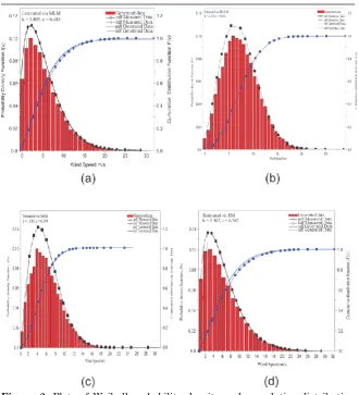
generated data having 7000 random variables. The histograms are overlapped by Weibull probability distribution function (pdf) and cumulative probability distribution function (cdf) calculated with specific shape and scale parameters for the actual wind speed data as well as for the generated data. These figures show a good agreement between the histograms, pdf and cdf of the actual time series data and of generated data where Weibull shape and scale parameters calculated using 4 statistical methods, i.e., MLM, MMLM, MoM and EM.
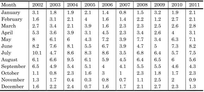
Table 1. Mean monthly wind speed (m/s) for Karachi at 0000 hours
Month 2002 2003 2004 2005 2006 2007 2008 2009 2010 2011
January 3.1 1.8 1.9 2.1 1.4 0.8 1.5 3.2 1.9 2.1
February 1.6 3.1 2.1 4 1.6 1.4 2.2 1.2 2.7 2.1
March 2.7 3.4 2.1 3.9 1.6 2.3 2.3 2.5 2.6 2.8
April 5.3 3.6 3.9 3.1 4.5 2.3 3.4 2.6 4 3.1
May 8 6.1 6 4.3 7.2 3.9 7.7 3.4 6.3 7.1
June 8.2 7.6 8.1 5.5 6.7 3.9 4.7 5 7.3 8.2
July 10.1 4.7 8.6 8.3 8.6 3.5 6.8 6.4 5.7 7.5
August 6.1 6.6 9.5 6.1 5.9 4.5 6.4 6.5 6 5.6
September 6.5 4.9 5.4 5.1 4 4.1 5.5 5.5 4.6 4.3
October 1.1 0.8 2.3 1.6 3 1 2.3 1.8 1.7 2.3
November 1.3 1.7 0.4 0.3 0.8 0.7 1.1 2.5 2 0.9
December 1.6 2.2 2.4 0.7 1.6 1.7 2.1 2.7 2.3 1.3
Table 2. Mean monthly wind speed (m/s) for Karachi at 1200 hours
Month 2002 2003 2004 2005 2006 2007 2008 2009 2010 2011
January 6 7.1 6.3 4.6 4.5 4 4.5 7.4 5 5.4
February 6.9 8.3 7.4 6.9 6 7.5 7.6 7.3 6.8 6.6
March 8.6 9.4 7.8 7.9 7.8 6.8 8.2 7.8 7.7 6.5
April 10.9 9.1 10.2 9.2 8.9 7.5 10.3 8.9 8.3 8
May 12.6 11.2 11.7 10.3 10.4 10.2 12.6 9.9 9.8 11.7
June 13.1 10.5 12.2 9.9 10.8 10.3 8.8 9.7 9.3 11.7
July 13.9 7.9 12.5 10.9 11.4 8.6 11 9.4 8.8 10.8
August 9.7 9.6 11.9 10.3 8.5 9.5 9.2 9.3 7.2 8.5
September 11 7.3 9.4 8.1 6.4 8 8.7 9 6.5 7.4
October 5.6 6.2 6.7 5.5 7.9 5.8 6.5 6.1 6.2 6.3
November 5.8 4.7 3.8 4.4 4 6.2 4.9 5 4.9 5.4
function parameters
Figure-1: Comparision of actual wind speed data with Weibull pdfs each with particular shape and scale parameters estimated by using four different numerical methods.
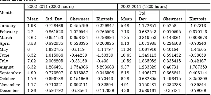
Table 3: Mean wind speed, wind speed standard deviation, skewness and Kurtosis
Month
2002-2011 (0000 hours) 2002-2011 (1200 hours)
Mean Std. Dev. Skewness Kurtosis Mean Std.
Figure 2: Plots of Weibull probability density and cumulative distribution function (a) Maximum likelihood method (b) Modified maximum likelihood method (c) Method of Moment (d) Empirical method
Table 4: Statistical Analysis
Numerical Method
Weibull Parameter Statistical Tests
k c (m/s) vm (m/s) Ed W/m2 RMSE 2 R2
MLE 0.475 1.260 2.755 1590.851 0.846 0.716 0.995
MLM 1.403 6.445 5.816 370.048 0.154 0.023 0.996
MMLM 2.258 8.852 7.763 499.228 0.347 0.120 0.996
MoM 1.818 6.559 5.773 254.253 0.323 0.104 0.996
EM 1.362 6.367 5.773 379.955 0.157 0.024 0.996
EPFM 1.366 218.263 197.828 1.521 x
107
function parameters
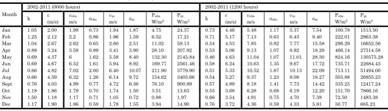
Table 5: Comparison between actual and estimated values of wind parameters for measured mean monthly k and c parameters using maximum likelihood method (MLM)
Month
2002-2011 (0000 hours) 2002-2011 (1200 hours) k c
(m/s)
vobs
m/s σobs
vm
m/s σm Pobs
W/m2
Pm
W/m2 k
c (m/s)
vobs
m/s σobs
vm
m/s σm Pobs
W/m2
Pm
W/m2
Jan 1.98 3.59 1.98 0.73 3.15 1.70 4.754 37.65 2.13 6.78 5.48 1.17 5.95 3.02 100.797 236.67 Feb 1.70 4.30 2.2 0.86 3.80 2.34 6.522 78.36 2.27 8.05 7.13 0.63 7.06 3.39 222.011 374.12 Mar 1.90 4.54 2.62 0.65 3.99 2.23 11.016 79.85 3.32 8.80 7.85 0.82 7.82 2.73 296.289 398.45 Apr 2.04 5.10 3.58 0.89 4.47 2.35 28.103 104.63 3.54 10.11 9.13 1.07 9.01 2.98 466.142 592.35 May 2.39 7.18 6 1.62 6.30 2.89 132.300 254.55 4.74 12.02 11.04 1.07 10.89 2.86 824.163 945.55 Jun 2.52 7.71 6.52 1.61 6.78 2.98 169.765 304.76 3.35 11.60 10.63 1.35 10.31 3.57 735.709 908.63 Jul 2.62 8.35 7.02 2.00 7.35 3.12 211.893 377.86 3.84 11.67 10.52 1.87 10.45 3.24 713.105 893.49 Aug 2.39 7.47 6.32 1.26 6.56 3.01 154.617 287.53 3.47 10.49 9.37 1.23 9.34 3.14 503.877 664.92 Sept 2.12 6.17 4.99 0.77 5.41 2.75 76.104 178.71 3.22 9.12 8.18 1.41 8.09 2.89 335.248 447.50 Oct 2.09 3.97 1.79 0.70 3.49 1.79 3.513 48.33 3.09 7.03 6.28 0.68 6.22 2.31 151.700 208.47 Nov 1.97 3.06 1.17 0.71 2.69 1.46 0.981 23.56 2.47 5.74 4.91 0.75 5.04 2.25 72.502 127.10 Dec 1.87 3.79 1.86 0.59 3.33 1.89 3.941 47.38 2.04 5.55 4.36 0.59 4.87 2.57 50.765 135.50
Table 6: Comparison between actual and estimated values of wind parameters for measured mean monthly k and c parameters using modified maximum likelihood method (MMLM)
Month
2002-2011 (0000 hours) 2002-2011 (1200 hours) k c (m/s) vobsm/s σobs vmm/s σm PW/mobs2
Pm
W/m2 k
c (m/s)
vobs
m/s σobs vmm/s σm PW/mobs2
Pm
W/m2
Jan 2.34 3.05 1.98 0.73 2.68 1.25 4.754 19.88 2.65 6.31 5.48 1.17 5.55 2.34 100.797 161.95 Feb 2.52 3.78 2.2 0.86 3.33 1.46 6.522 36.00 2.96 7.90 7.13 0.63 6.98 2.68 222.011 301.06 Mar 3.06 4.22 2.62 0.65 3.73 1.39 11.016 45.07 4.18 8.42 7.85 0.82 7.58 2.20 296.289 330.60 Apr 2.46 4.75 3.58 0.89 4.17 1.87 28.103 72.40 4.94 9.71 9.13 1.07 8.82 2.24 466.142 496.95 May 2.84 6.89 6 1.62 6.08 2.41 132.300 203.11 5.86 11.60 11.04 1.07 10.64 2.38 824.163 838.92 Jun 3.22 7.27 6.52 1.61 6.45 2.31 169.765 227.03 4.24 11.14 10.63 1.35 10.03 2.87 735.709 764.16 Jul 3.04 7.85 7.02 2.00 6.94 2.60 211.893 291.60 4.89 11.20 10.52 1.87 10.16 2.60 713.105 761.87 Aug 2.99 7.19 6.32 1.26 6.36 2.42 154.617 225.76 4.55 10.05 9.37 1.23 9.08 2.46 503.877 554.61 Sept 2.61 5.54 4.99 0.77 4.87 2.08 76.104 110.54 4.29 8.81 8.18 1.41 7.94 2.25 335.248 376.52 Oct 2.54 3.38 1.79 0.70 2.97 1.30 3.513 25.48 3.75 6.56 6.28 0.68 5.87 1.86 151.700 159.82 Nov 1.73 2.25 1.17 0.71 1.99 1.21 0.981 11.03 3.39 5.36 4.91 0.75 4.77 1.64 72.502 89.58 Dec 2.93 3.49 1.86 0.59 3.08 1.19 3.941 26.08 2.62 5.44 4.36 0.59 4.79 2.03 50.765 104.38
Table 7: Comparison between actual and estimated values of wind parameters for measured mean monthly k and c parameters using method of moments (MoM)
Month
2002-2011 (0000 hours) 2002-2011 (1200 hours) k c (m/s) vobsm/s σobs vmm/s σm PW/mobs2
Pm
W/m2 k
c (m/s)
vobs
m/s σobs vmm/s σm PW/mobs2
Pm
W/m2
Table 8: Comparison between actual and estimated values of wind parameters for measured mean monthly k and c parameters using empirical method (EM)
Month
2002-2011 (0000 hours) 2002-2011 (1200 hours) k c (m/s) vobsm/s σobs vmm/s σm PW/mobs2
Pm
W/m2 k
c (m/s)
vobs
m/s σobs vmm/s σm PW/mobs2
Pm
W/m2
Jan 0.98 1.91 1.98 0.73 1.91 1.97 4.754 27.67 1.72 6.15 5.48 1.17 5.43 3.31 100.797 225.95 Feb 0.74 1.62 2.2 0.86 1.92 2.65 6.522 65.07 1.82 7.33 7.13 0.63 6.45 3.75 222.011 354.98 Mar 0.93 2.50 2.62 0.65 2.56 2.78 11.016 76.03 3.14 8.86 7.85 0.82 7.85 2.87 296.289 414.79 Apr 1.22 3.72 3.58 0.89 3.45 2.88 28.103 99.39 3.16 10.09 9.13 1.07 8.94 3.25 466.142 611.44 May 2.06 6.74 6 1.62 5.91 3.09 132.300 240.08 4.96 12.17 11.04 1.07 11.06 2.80 824.163 977.79 Jun 2.03 7.11 6.52 1.61 6.24 3.30 169.765 285.39 2.96 11.46 10.63 1.35 10.12 3.89 735.709 917.11 Jul 2.34 7.90 7.02 2.00 6.93 3.24 211.893 344.96 3.82 11.73 10.52 1.87 10.50 3.26 713.105 908.00 Aug 2.12 7.16 6.32 1.26 6.28 3.20 154.617 279.54 3.20 10.53 9.37 1.23 9.33 3.35 503.877 690.07 Sept 1.61 5.41 4.99 0.77 4.80 3.09 76.104 169.07 2.78 8.97 8.18 1.41 7.91 3.19 335.248 453.09 Oct 0.77 1.54 1.79 0.70 1.78 2.35 3.513 45.46 2.99 7.08 6.28 0.68 6.26 2.38 151.700 215.03 Nov 0.67 0.87 1.17 0.71 1.14 1.76 0.981 19.82 2.06 5.40 4.91 0.75 4.74 2.47 72.502 123.07 Dec 0.85 1.68 1.86 0.59 1.81 2.16 3.941 34.79 1.57 4.88 4.36 0.59 4.34 2.88 50.765 130.34
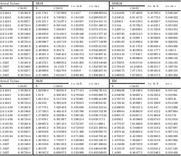
Table 9: Relative errors (r.e.) for Weibull parameters (k and c) between actual and simulated data, 100 data points repeated 100 times using Monte Carlo.
Actual Values MLM
r.e. in k r.e. in c MMLM r.e. in k r.e. in c
K c (m/s) k c (m/s) k c (m/s)
2.24245 7.503619 2.611781 7.727896 0.1647 0.029889304 3.224495 7.874636 0.437934 0.049445 2.24245 8.503468 2.611418 8.748925 0.164538 0.028865557 3.224021 8.914375 0.437723 0.048322 2.24245 6.559257 2.612311 6.712974 0.164937 0.023435113 3.26565 6.841593 0.456287 0.043044 2.24245 6.367244 2.609937 6.591046 0.163878 0.035148813 3.2344 6.707923 0.442351 0.053505 2.611459 7.503619 2.689686 7.558001 0.029955 0.007247554 3.429514 7.686365 0.313256 0.024354 2.611459 8.503468 2.688356 8.514843 0.029446 0.001337743 3.436795 8.695123 0.316044 0.022539 2.611459 6.559257 2.694336 6.606199 0.031736 0.007156511 3.419146 6.729811 0.309286 0.026002 2.611459 6.367244 2.695967 6.416749 0.032361 0.007774896 3.408163 6.538092 0.30508 0.026832 1.818194 7.503619 2.489208 8.130331 0.369055 0.083521363 2.921081 8.211702 0.606584 0.094366 1.818194 8.503468 2.483928 9.30472 0.366151 0.094226567 2.930523 9.405939 0.611777 0.10613 1.818194 6.559257 2.482514 7.048452 0.365373 0.074580741 2.981245 7.179457 0.639674 0.094553 1.818194 6.367244 2.486759 6.855543 0.367708 0.076689113 2.97089 6.998606 0.633978 0.099158 1.3627 7.503619 2.263721 8.868932 0.661203 0.181954068 2.570201 8.945704 0.886109 0.192185 1.3627 8.503468 2.269059 10.15617 0.66512 0.194356758 2.578443 10.20206 0.892157 0.199752 1.3627 6.559257 2.269986 7.822706 0.6658 0.192620734 2.568575 7.871795 0.884916 0.200105 1.3627 6.367244 2.274899 7.612847 0.669405 0.19562655 2.566203 7.676235 0.883175 0.205582 Actual Values MoM
r.e. in k r.e. in c EM r.e. in k r.e. c
k c (m/s) k c (m/s) k c (m/s)
function parameters
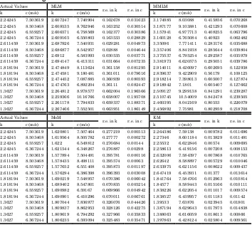
Table 10: Relative errors (r.e.) for Weibull parameters (k and c) between actual and simulated data, 1000 data points repeated 100 times using Monte Carlo.
Actual Values MLM
r.e. in k r.e. in c MMLM r.e. in k r.e. in c
k c (m/s) k c (m/s) k c (m/s)
2.24245 7.503619 2.607247 7.740904 0.162678 0.031623 3.174985 8.03088 0.415856 0.070268 2.24245 8.503468 2.608535 8.762946 0.163252 0.030514 3.187177 9.103881 0.421293 0.070608 2.24245 6.559257 2.606571 6.758569 0.162377 0.030386 3.157941 6.977713 0.408255 0.063796 2.24245 6.367244 2.609165 6.550803 0.163533 0.028829 3.160128 6.765084 0.40923 0.062482 2.611459 7.503619 2.687926 7.540931 0.029281 0.004973 3.35096 7.771411 0.283176 0.035688 2.611459 8.503468 2.686877 8.542957 0.02888 0.004644 3.357406 8.841938 0.285644 0.039804 2.611459 6.559257 2.6912 6.583993 0.030535 0.003771 3.375537 6.795254 0.292587 0.035979 2.611459 6.367244 2.694147 6.413311 0.031664 0.007235 3.381973 6.620575 0.295051 0.039786 1.818194 7.503619 2.474849 8.113624 0.361158 0.081295 2.914011 8.426097 0.602695 0.122938 1.818194 8.503468 2.474581 9.180481 0.361011 0.079616 2.839637 9.422909 0.56179 0.108125 1.818194 6.559257 2.474452 7.087885 0.360939 0.080593 2.918214 7.398013 0.605007 0.127874 1.818194 6.367244 2.474763 6.892204 0.36111 0.082447 2.918942 7.1801 0.605407 0.127662 1.3627 7.503619 2.264812 8.978577 0.662004 0.196566 2.509127 9.299138 0.841291 0.239287 1.3627 8.503468 2.259366 10.16766 0.658007 0.195708 2.510745 10.54009 0.842478 0.239505 1.3627 6.559257 2.261178 7.794833 0.659337 0.188371 2.460395 8.042169 0.80553 0.226079 1.3627 6.367244 2.267466 7.552501 0.663951 0.186149 2.456892 7.75981 0.802959 0.218708
Actual Values MoM
r.e. in k r.e. in c EM r.e. in k r.e. in c
k c (m/s) k c (m/s) k c (m/s)
2.24245 7.503619 1.620801 7.507464 0.277219 0.000513 2.264386 7.59138 0.009782 0.011696 2.24245 8.503468 1.619564 8.505782 0.27777 0.000272 2.27346 8.601184 0.013829 0.011491 2.24245 6.559257 1.622 6.549812 0.276684 0.00144 2.25532 6.622846 0.00574 0.009695 2.24245 6.367244 1.621544 6.348267 0.276887 0.00298 2.258613 6.419156 0.007208 0.008153 2.611459 7.503619 1.577894 7.504491 0.395781 0.000116 2.632006 7.584397 0.007868 0.010765 2.611459 8.503468 1.578435 8.498111 0.395574 0.00063 2.62642 8.588897 0.005729 0.010046 2.611459 6.559257 1.577652 6.551408 0.395873 0.001197 2.633975 6.621156 0.008622 0.009437 2.611459 6.367244 1.576294 6.386398 0.396393 0.003008 2.647419 6.453931 0.01377 0.013614 1.818194 7.503619 1.690219 7.548957 0.070386 0.006042 1.841764 7.584766 0.012963 0.010814 1.818194 8.503468 1.689402 8.547801 0.070835 0.005214 1.84577 8.589443 0.015166 0.010111 1.818194 6.559257 1.690982 6.59167 0.069966 0.004942 1.838226 6.622054 0.011017 0.009574 1.818194 6.367244 1.690901 6.410296 0.070011 0.006761 1.838527 6.439957 0.011183 0.01142 1.3627 7.503619 1.807044 7.836977 0.326076 0.044426 1.39533 7.63876 0.023945 0.01801 1.3627 8.503468 1.809837 8.862953 0.328126 0.042275 1.387194 8.629643 0.017975 0.014838 1.3627 6.559257 1.809619 6.794292 0.327966 0.035833 1.388063 6.616059 0.018613 0.00866 1.3627 6.367244 1.806235 6.593094 0.325483 0.035471 1.397863 6.428124 0.025804 0.009561
Table 11: Relative errors (r.e.) for Weibull parameters (k and c) between actual and simulated data, 10000 data points repeated 100 times using Monte Carlo.
Actual Values MLM
r.e. in k r.e. in c MMLM r.e. in k r.e. in c
k c (m/s) k c (m/s) k c (m/s)
2.611459 6.367244 2.689218 6.396995 0.029776 0.004672 3.358803 6.646466 0.286179 0.043853 1.818194 7.503619 2.47443 8.109489 0.360927 0.080744 2.855737 8.434634 0.570645 0.124076 1.818194 8.503468 2.473158 9.182419 0.360228 0.079844 2.855558 9.551758 0.570546 0.123278 1.818194 6.559257 2.476066 7.089611 0.361827 0.080856 2.855833 7.37261 0.570697 0.124001 1.818194 6.367244 2.476345 6.877256 0.361981 0.080099 2.855377 7.15179 0.570447 0.123216 1.3627 7.503619 2.257541 8.963197 0.656668 0.194517 2.437924 9.231691 0.78904 0.230299 1.3627 8.503468 2.257345 10.15133 0.656524 0.193787 2.438641 10.45648 0.789566 0.229672 1.3627 6.559257 2.258127 7.831833 0.657097 0.194012 2.437938 8.064243 0.78905 0.229445 1.3627 6.367244 2.257738 7.600787 0.656813 0.193733 2.436084 7.825456 0.787689 0.229018
Actual Values MoM
r.e. in k r.e. in c EM r.e. in k r.e. in c
k c (m/s) k c (m/s) k c (m/s)
2.24245 7.503619 1.620515 7.500672 0.277346 0.000393 2.265451 7.584887 0.010257 0.010831 2.24245 8.503468 1.620522 8.500671 0.277343 0.000329 2.265296 8.596144 0.010188 0.010899 2.24245 6.559257 1.621024 6.55471 0.277119 0.000693 2.261605 6.628227 0.008542 0.010515 2.24245 6.367244 1.620972 6.356754 0.277142 0.001648 2.261946 6.428073 0.008694 0.009553 2.611459 7.503619 1.57874 7.497464 0.395457 0.00082 2.622355 7.577897 0.004172 0.009899 2.611459 8.503468 1.578553 8.499585 0.395528 0.000457 2.624223 8.590679 0.004888 0.010256 2.611459 6.559257 1.578791 6.554773 0.395437 0.000684 2.621822 6.625115 0.003968 0.01004 2.611459 6.367244 1.578737 6.36083 0.395458 0.001007 2.62233 6.429078 0.004163 0.009711 1.818194 7.503619 1.689957 7.54617 0.07053 0.005671 1.842286 7.582641 0.013251 0.010531 1.818194 8.503468 1.690048 8.544944 0.07048 0.004878 1.841836 8.58612 0.013003 0.00972 1.818194 6.559257 1.68992 6.596077 0.07055 0.005613 1.842481 6.627991 0.013358 0.010479 1.818194 6.367244 1.690016 6.397864 0.070497 0.004809 1.842003 6.428722 0.013095 0.009655 1.3627 7.503619 1.810884 7.806965 0.328894 0.040427 1.383487 7.59918 0.015254 0.012735 1.3627 8.503468 1.810966 8.841407 0.328954 0.039741 1.383365 8.60575 0.015165 0.012028 1.3627 6.559257 1.811117 6.8196 0.329065 0.039691 1.382936 6.637436 0.01485 0.011919 1.3627 6.367244 1.811272 6.618481 0.329179 0.039458 1.382478 6.441339 0.014514 0.011637
function parameters
using the theoretical model. From the statistical analysis the values of RMSE, 2 and R2 are consistent for the estimation methods MLM, MMLM, MoM and EM. For MLE both RMSE and 2-test give comparatively large values, i.e. 0.846 and 0.716, respectively, indicating a less probable fit. Although for EPFM both RMSE and 2-test gives small values, i.e., 0.153 and 0.023, respectively but the mean Weibull speed is much higher than monthly mean measured wind speeds. Inspection of table 5 to 8 indicate that the estimated mean monthly wind speeds are in good agreement with the actual mean monthly wind speeds.
4. Conclusions
5. Acknowledgement
The authors are thankful to the Karachi Metrological Office for providing the measured wind speed data for the analysis. The authors are also thankful to Prof. Dabir Hassan Rizvi for his critical comments. This study was financially supported by the University of Karachi through the Dean Faculty Science grant.
REFERENCES
Smil, V. 2006. “Energy at the crossroads.” Paper presented at OECD Global Science Forum, 17-18 May 2006, Paris. [1] Weibull, W. 1951. "A statistical distribution function of wide
applicability." J. Appl. Mech.-Trans. ASME 18 (3): 293– 297. [2]
Carta, J.A., Ramirez, P., and Velazquez, S. 2009. “A review of wind speed probability distributions used in wind energy analysis case studies in the Canary Islands.” Renewable
and Sustainable Energy Reviews 13: 933–955. [3]
Sopian, K., Othman, M. Y. H., and Wirsat, A. 1995. “Data Bank, the wind energy potential of Malaysia.”
Renewable Energy 6(8): 1005-1016. [4]
Garcia, A., Torres, J. L., Prieto, E., and Francisco, A. D. 1998. “Fitting wind speed distributions: A case study.” Solar energy 62(2): 139-l 44. [5]
Sulaiman, M.Y., Akaak, A.M., Wahab, M.A., Zakaria, A., Sulaiman, Z. A., and Suradi, J. 2002. “Wind Characteristics of Oman.” Energy 27: 35-46. [6]
Seguro, J. V. and Lambert, T. W. 2000. “Modern Estimation of parameters of the Weibull wind speed distribution for wind energy analysis.” Journal of Wind Engineering and
Industrial aerodynamics 85: 75-84. [7]
function parameters
for electricity in a land aquafarm in Taiwan.” Renew
Energy 31:877–92. [8]
Zhou, W, Yang, H.X., and Fang, Z.H. 2006. “Wind power potential and characteristic analysis of the Pearl River Delta region, China.” Renew Energy 31:739–53. [9] Akpinar, E.K. and Akpinar, S. 2004. “Determination of the
wind energy potential for Maden-Elazig, Turkey.”
Energy Convers Manage 45:2901–14. [10]
Celik, A.N. 2003. “A statistical analysis of wind power density based on the Weibull and Rayleigh models at the southern region of Turkey.” Renew Energy 29:593–604. [11]
Ucar, A. and Balo, F. 2009. “Investigation of wind characteristics and assessment of wind generation potentiality in Uludag-Bursa, Turkey.” Appl Energy
86:333–9. [12]
Chang, T.J., Wu, Y.T., Hsu, H.Y., Chu, C.R., Liao, C.M. 2003. “Assessment of wind characteristics and wind turbine characteristics in Taiwan.” Renew Energy 28:851–71. [13]
Kwon, S.D. 2010. “Uncertainty analysis of wind energy potential assessment.” Appl Energy 87: 856–65. [14] Thiaw, L., Sow, G., Fall, S.S., Kasse, M., Sylla, E., Thioye, S.
2010. “A neural network based approach for wind resource and wind generators production assessment.”
Appl Energy 87: 1744–8. [15]
Seguro, J.V. and Lambert, T.W. 2000. “Modern estimation of the parameters of the Weibull wind speed distribution for wind energy analysis.” J Wind Eng Ind Aerod 85:75– 84. [16]
Akdag, S.A. and Dinler, A. 2009. “A new method to estimate Weibull parameters for wind energy applications.”
Energy Convers Manage 50:1761–6. [17]
Energy 86:538–45. [18]
Dorvlo, A.S.S. 2002. “Estimating wind speed distribution.”
Energy Convers Manage 43:2311–8. [19]
Ghosh, A. 1999. “A FORTRAN program for fitting Weibull distribution and generating samples.” Comput Geosci
25:729–38. [20]
Genc, A, Erisoglu, M, Pekgor, A, Oturanc, G, Hepbasli, A, and Ulgen K. 2005. “Estimation of wind power potential using Weibull distribution.” Energy Sources 27:809–22. [21]
Kantar, YM, Senoglu, B. 2008. “A comparative study for the location and scale parameters of the Weibull distribution with given shape parameter.” ComputGeosci 34:1900–9. [22]
Lun, Isaac Y. F. and Lam, Joseph C. 2000. "A Study of Weibull Parameters Using Long-Term Wind Observations",
Renewable Energy. 20(2), pp 145-153. [23]
Justus, CG, Hargraves, WR, Mikhail, A, and Graber, D. 1978. “Methods for estimating wind speed frequency distributions.” Journal of Applied Meteorology 17:350-3. [24]
Barthelmie, R.J. and S.C. Pryor. 2003. “Can satellite sampling of offshore wind speeds realistically represent wind speed distribution.” Journal of Applied Meteorology 42: 83-94. [25]
Keyhani, A, Ghasemi-Varnamkhasti, M, Khanali, M, and Abbaszadeh, R. 2010. “An assessment of wind energy potential as a power generation source in the capital of Iran, Tehran.” Energy 35(1):188e201. [26]
Stevens, M.J. and P.T. Smulders. 1979. “The estimation of the parameters of the Weibull wind speed distribution for wind energy utilization purposes.” Wind Engineering
3(2): 132-145. [27]
function parameters
for Wind Energy Analysis." Journal of Wind Engineering
and Industrial Aerodynamics. 85(1): 75-84. [28]
Pearson, K. 1936. “Method of moments and method of maximum likelihood.” Biometrika 28: 34-59. [29]
Bridgman, Percy W., Gerald Holton. "Empirical method." In AccessScience@McGraw-Hill. [30]
Akdag, SA and Dinler, A. 2009. “A new method to estimate Weibull parameters for wind energy applications.”
Energy Convers Manage 50:1761-6. [31]
Raichle, BW and Carson WR. 2009. “Wind resource assessment of the Southern Appalachian Ridges in the Southeastern United States.” Renew Sust Energy Rev 13:1104-10. [32] Wichmann, B. A. and I. D. Hill. 1982. “Algorithm AS 183: An
Efficient and Portable Pseudo-Random Number
Generator.”Applied Statistics 31(2): 188-190. [33]
Hahn, G.J. and Shapiro, S.S. 1967. Statistical Models in
Engineering. New York: John Wiley and Sons. [34]