The International Comparison Project as a Source of Private Consumption Data for a Global Input-Output Model

(1)

Telephone: from overseas: (03) 9905 2398, (03) 9905 5112 61 3 9905 2398 or 61 3 9905 5112

Fax: (03) 9905 2426 from overseas: 61 3 9905 2426

e-mail [email protected]

The International Comparison

Project as a Source of Private

Consumption Data for a Global

Input-Output Model

by

G. A. M

EAGHER

Centre of Policy Studies

Monash University

Preliminary Working Paper No. IP-62 Dec 1993

ISSN 1031 9034

ISBN0 642 10337 2

The Centre of Policy Studies and Impact Project is a research centre at Monash University devoted to quantitative analysis of issues relevant to Australian economic policy.

C

ENTRE

of

P

OLICY

S

TUDIES

and

the

I

MPACT

(2)

i

In 1989 a major project entitled "Strategies for Environmentally Sound Economic Decelopment" was inaugurated under the sponsorship of the United Nations. This project is designed to identify ways of alleviating pressures on the global environment and, at the same time, raise the standard of living of the poorest countries. The central component of its analytical framework is a dynamic global input-output model (GIOM) that describes trade between 15 regions in about 50 commodities, taking as its starting point the well known 1977 World Input-Output Model of Leontief, Carter and Petri.

The purpose of the present paper is twofold. Firstly, it describes a contribution to the compilation of a database for the GIOM. In particular, it draws on data collected by the United Nations' International Comparison Project (ICP) to provide estimates of private consumption expenditure for 1980, the base period for the model. Secondly, it uses these estimates as a case study to examine the implications of using different price systems for each country, rather than a common set of prices, to determine expenditures on composite commodities. In preparing data for multisectoral global models, it is common practice to collect expenditure data evaluated in local (national) prices and convert to world prices using published exchange rates. The analysis of this paper suggests that, when commodities produced in different countries are treated as perfect substitutes in the model, the practice may seriously compromise the model's results.

(3)

ii

1 Introduction 1

2 Estimates of GDP Based on Domestic Prices 2

2.1 The ICP Data 2

2.2 Conversion of the ICP Data to the

GIOM Commodity Classification 4

2.3 Conversion of the ICP Data to the

GIOM Regional Classification 6

3 Estimates of GDP Based on International and

Regional Prices 11

4 Interpretation and Assessment of GDP Estimates 16

5 Concluding Remarks 21

(4)

iii

1 The GIOM Expenditure Classification 5

2 Judgmental Allocation Rules Employed in the

Commodity Classification Conversion 7

3 The GIOM Classification of Regions 8

4 Gross Domestic Product, MEDS Data, 1980,

Newly-industrializing Latin America 8

5 Gross Domestic Product, Weighted ICP Data,

1980, Domestic Prices, $US 10

1980, International Prices, $I 13

1980, Regional Prices, $R 15

8 Deviations Between Expenditures Measured in

(5)

by G.A. Meagher*

Centre of Policy Studies Monash University

1. Introduction

In the mid-1970's, the United Nations sponsored the development of an input-output model of the world economy (Leontief et al., 1977) designed to investigate the interrelationships between environmental and other economic policies proposed for the remainder of the 20th century. The Leontief model can be regarded as the forerunner of a string of other global multisectoral models, including the computable general equilibrium (CGE) models of Whalley (1985), Deardorf and Stern (1986), Mercenier and Waelbroeck (1986), Burniaux et al. (1989) and Zeitsch et al. (1991). More directly, it provided the starting point for the recent work, also sponsored by the United Nations, of Duchin et al. (1992, 1994) on strategies for environmentally sound economic development. The central component of their analytical framework is a dynamic global input-output model (GIOM) specified in the first instance as a revised version of the Leontief model.

A common feature of all these models is that they incorporate international trade in composite commodities produced in different countries. Hence the construction of their databases involves the use of price systems whereby expenditures on unlike components are added together to obtain expenditures on the specified composites. For want of an alternative, it is usual to employ each country's own price system to determine composite expenditures in local currency. These expenditures are then converted to a common currency using published exchange rates.

*_{The author is indebted to Faye Duchin and Brian Parmenter for comments on previous}

(6)

The purpose of the present paper is twofold. Firstly, it describes a contribution to the compilation of a database for the GIOM of Duchin et al. In particular, it draws on data collected by the United Nations' International Comparison Project (ICP) to provide estimates of private consumption expenditure for 1980, the base period for the model. Secondly, it uses these estimates as a case study to examine the implications of using different price systems for each country, rather than a common set of prices, to determine expenditures on composite commodities. While the estimates themselves may be too outdated to be of direct use for other purposes, the procedures employed in their construction and the issues raised by the differences between them are of continuing importance.

The balance of the paper is organized as follows. Section 2 describes the ICP database and the methodology for converting it to the commodity classification of the GIOM. It then employs data from the United Nations' Macroeconomic Data System (MEDS) to convert the ICP data to the GIOM regional classification. The consumption estimates resulting from these procedures incorporate the domestic prices of the ICP countries converted to US dollars using published exchange rates. In Section 3, two alternative estimates are described, one based on a set of average world prices computed as part of the ICP and the other based on sets of average prices for the GIOM regions. In Section 4, the various estimates are interpreted and assessed. Section 5 contains some brief concluding remarks.

2. Estimates of GDP Based on Domestic Prices

2.1 The ICP Data

The International Comparison Project has been producing estimates of purchasing power parities (PPPs) and of real gross domestic product (GDP) and its components for the last 20 years. The project has proceeded through five phases corresponding to the reference years 1970, 1973, 1975, 1980 and 1985, respectively.1_{The consumption estimates reported in this paper are derived from}

1_{A comprehensive report on Phase III, together with references to earlier work, is}

(7)

unpublished Phase IV data supplied by the ICP Section of the United Nations Statistical Office.2

The data was supplied in the form of five tables which will be referred to as Tables IV.1 to IV.5. The first contains estimates Ein of expenditure of type i in country n for 60 countries and 151 expenditure types (or "basic headings"). If the expenditures Ein are summed over expenditure types, one obtains the GDP of country n. The expenditures in Table IV.1 are expressed in domestic currencies, but they can be converted to US dollars using exchange rates included in Table IV.4 (see below).

Table IV.2 contains the price ratios or purchasing power parities

P ^

in = Pin / Pi,US (i=1,...,151; n=1...,60)

where P_in is the price of expenditure type or "commodity" i in country n. When an element of Table IV.1 is divided by the corresponding element of Table IV.2, one obtains the expenditure

Q^_in = P_i,US Q_in

where Q_in is the amount of commodity i purchased in country n. Note that

E_in = P^_in Q^_in = P_in Q_in .

Table IV.3 contains per capita expenditures EI_in / N_n , where N_n is the population of country n and the expenditures EI_in are expressed in terms of a set PI_i of world prices whose derivation is discussed in Section 3. Table IV.4 contains values of the exchange rate R_n with respect to the US dollar, the population N_n and a so-called "supercountry weight" W_n for each country. The final table of the database, Table IV.5, contains the information required to aggregate to the

2_{Some Phase IV results appear in two reports published by the United Nations in 1986}

(8)

commodity classification used in the reports published by the United Nations (1986 and 1987). Table IV.5 is not used for any purpose in this study.

2.2 Conversion of the ICP Data to the GIOM Commodity Classification

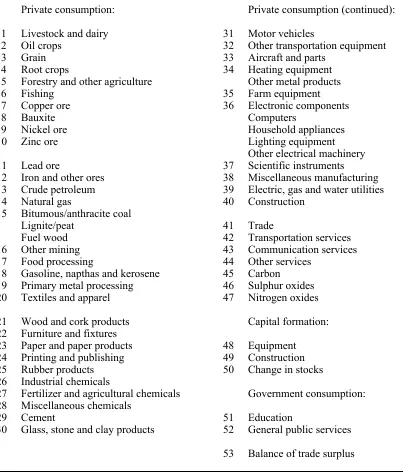
The GIOM classification of commodities consists of the first 47 categories of the expenditure classification set out in Table 1. Each of the commodity groups 1 to 44 is an aggregation of commodities defined at the 6-digit level of the International Standard Industrial Classification (ISIC).3_{Commodities 45 to 47 are not defined in}

ISIC, but are included in the GIOM to facilitate aspects of environmental modelling. These 47 categories are designed to cover all uses of commodities in the GIOM, i.e., intermediate usage, capital formation, private consumption, government consumption and international trade. However, bearing in mind the requirements of mobilizing the ICP data and the focus of the present study on private consumption, it is convenient to define separate categories for uses other than private consumption, i.e., to include the expenditure categories 48 to 53. This treatment means that many of the standard GIOM commodities (namely, all those that are not directly consumed by the private sector) do not appear in the analysis that follows.

The task of converting the ICP data to the GIOM commodity classification, then, consists of assigning each of the 151 ICP basic headings to one or more of the 53 expenditure types in Table 1. The procedure involves three steps, the first of which is to assign ISIC categories to the basic headings. The assignment was based on a comparison of verbal descriptions of the basic headings published by EUROSTAT (1983) with verbal descriptions of the ISIC categories contained in two United National publications (1971a and 1971b). The ICP tables themselves also contain verbal descriptions of the basic headings but they are often too terse to be useful for the current purpose.

Once the basic headings have been associated with ISIC categories, they can be assigned to GIOM expenditure types using the appropriate classification conversion (see footnote 3). This assignment constitutes step two of the conversion procedure.

3_{The conversion between GIOM and ISIC commodities has been published in various}

(9)

Table 1. The GIOM Expenditure Classification

No. Description No. Description

Private consumption: Private consumption (continued):

1 Livestock and dairy 31 Motor vehicles

2 Oil crops 32 Other transportation equipment 3 Grain 33 Aircraft and parts

4 Root crops 34 Heating equipment 5 Forestry and other agriculture Other metal products 6 Fishing 35 Farm equipment 7 Copper ore 36 Electronic components

8 Bauxite Computers

9 Nickel ore Household appliances 10 Zinc ore Lighting equipment

Other electrical machinery 11 Lead ore 37 Scientific instruments

12 Iron and other ores 38 Miscellaneous manufacturing 13 Crude petroleum 39 Electric, gas and water utilities 14 Natural gas 40 Construction

15 Bitumous/anthracite coal

Lignite/peat 41 Trade

Fuel wood 42 Transportation services 16 Other mining 43 Communication services 17 Food processing 44 Other services

18 Gasoline, napthas and kerosene 45 Carbon 19 Primary metal processing 46 Sulphur oxides 20 Textiles and apparel 47 Nitrogen oxides

21 Wood and cork products Capital formation: 22 Furniture and fixtures

23 Paper and paper products 48 Equipment 24 Printing and publishing 49 Construction 25 Rubber products 50 Change in stocks 26 Industrial chemicals

27 Fertilizer and agricultural chemicals Government consumption: 28 Miscellaneous chemicals

29 Cement 51 Education

30 Glass, stone and clay products 52 General public services

(10)

Unfortunately, the procedure described thus far does not always result in a clear correspondence between ICP basic headings and GIOM expenditure types. In a number of cases, the basic heading corresponds to more than one GIOM category and a further allocation is required. Occasionally, the basic heading is so broadly defined that the corresponding GIOM categories are not obvious; basic heading 107, for example, is described as Musical instruments, boats and other major

durable goods. The third step in the conversion procedure, therefore, is to resolve

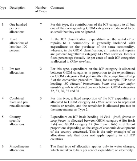
these ambiguities on the basis of informed judgment. In this case, the author's judgment was informed by discussions with Professor Alan Heston at the University of Pennsylvania (one of the originators of the ICP) and with Professor Faye Duchin and her team at New York University (who are responsible for the development of GIOM), as well as by his own experience in multi-sectoral modelling. The allocations performed at step 3 are summarized in Table 2.

The outcome of the three-step procedure is a table (not reported here) containing the expenditures Ein / Rn (i.e., the expenditures of Table IV.1 converted to US dollars), where the commodity index i now runs over the 53 expenditure types of Table 1 rather than the 151 types of Table IV.1.

2.3 Conversion of the ICP Data to the GIOM Regional Classification

The GIOM regional classification groups 189 countries into the 15 regions set out in Table 3.4_{The conversion of the expenditure data derived in section 2.2 from}

the 60 country ICP classification to the GIOM's 15 regions is based on information from the United Nation's MEDS database. Specifically, the MEDS database contains estimates of GDP in 1980 for 135 market economies which can be aggregated to obtain corresponding estimates for the GIOM regions. There are two things to note about this aggregation. First, the MEDS database contains no data for the centrally-planned economies of regions 6, 7 and 8. Second, even among the market economies, not all the countries belonging to the GIOM regions are included in MEDS. However, in the latter case, the countries omitted are quite small and the coverage in terms of regional GDP is high.

4_{The assignment of countries to regions in the GIOM has been published in various}

(11)

Table 2. Judgemental Allocation Rules Employed in the Commodity Classification Conversion

Type Description Number Comment of Cases

1 One hundred per cent allocations

7 For this type, the contributions of the ICP category to all but one of the corresponding GIOM categories are deemed to be so small that they can be ignored.

2 Fixed

allocations of less than 100 percent

6 In the ICP classification, expenditure on the rental of or repairs to a commodity is generally included with expenditure on the purchase of the same commodity, whereas, in the GIOM classification, all rentals and repairs are gathered togrether in category 44 Other services. Hence a fixed percentage (usually 10 per cent) of such ICP categories is allocated to Other services.

3 Pro rata

allocations 2 For this type, expenditure on the ICP category is allocatedbetween GIOM categories in proportion to the expenditures on GIOM categories that pertain after the completion of step 2 of the conversion procedure. Thus, for example, ICP basic heading 107 Musical instruments, boats and other major durable goods is allocated pro rata between GIOM categories 32, 33, 36, 37 and 38.

4 Combined fixed and pro rata allocations

3 For this type, a fixed proportion of the ICP expenditure is allocated to GIOM category 44 Other services to represent rentals or repairs, and the remainder is allocated pro rata in the same manner as Type 2.

5 Country specific allocations

1 Expenditure on ICP basic heading 14 Fish - fresh, frozen or deep frozen is allocated between GIOM category 6 (for fresh fish) and GIOM category 17 (for frozen fish) in different proportions depending on the stage of economic development of the country concerned. This is the only example of an allocation rule that does not apply equally in all ICP countries.

6 Miscellaneous

(12)

Table 3. The GIOM Classification of Regions

Region Code Description Number of Countries

1 NAH High-income North America 5 2 LAM Newly-industrializing Latin America 5 3 LAL Low-income Latin America 40 4 WEH High-income Western Europe 23 5 WEM Medium-income Western Europe 8

6 EEM Eastern Europe 7

7 RUH Soviet Union 1

8 CPA Centrally-planned Asia 3

9 JAP Japan 1

10 ASL Other Asia 23

11 OIL Major oil producers 15 12 AAF Other Middle-East and Northern Africa 16 13 SSA Sub-Saharan Africa 37

14 SAF Southern Africa 2

15 OCH Oceania 3

All regions 189

Table 4. Gross Domestic Product, MEDS Data, 1980, $USx106_{, Region LAM}

No. Country MEDS Code ICP Code GDP

1 Argentina 3 44 154011

2 Brazil 13 46 238490

3 Chile 23 47 27949

4 Mexico 79 194762

5 Venezuela 129 59 59171

(13)

To achieve the regional conversion, each ICP country is assigned a "supercountry weight", W*_n. Then the expenditure on commodity i in region m is determined as a weighted sum of the corresponding expenditures in the ICP countries belonging to region m. The method is illustrated for the second GIOM region, Newly-industrializing Latin America (LAM), which contains the five countries shown in Table 4. Four of these countries , i.e., all except Mexico, are ICP countries so expenditure on commodity i in region LAM is given by

E_i,44 W*₄₄ + E_i,46 W*₄₆ + E_i,47 W*₄₇ + E_i,59 W*₅₉ .

The supercountry weight is the same for each ICP country in the region and is given by the ratio of the regional GDP to the sum of the GDPs of all the ICP countries belonging to the region5_{, i.e.,}

W₄₄* = W*₄₆= W*₄₇ = W*₅₉

= 674383 / 47962= 1.406 .

Values of the supercountry weights are calculated in this manner for all the ICP countries except the centrally planned economies of Hungary and Poland which are not included in the MEDS database.

Table 5 contains estimates of GDP and its components in the desired categories of the GIOM. Only 10 of the 15 regions appear in the table, reflecting the fact that regions RUH (Soviet Union), CPA (Centrally-Planned Asia), SAF (Southern Africa) and OCH (Oceania) do not contain any ICP countries. The region EEM (Eastern Europe) contains two ICP countries - Hungary and Poland - but, as already mentioned, no supercountry weights are available for these countries from the databases considered in the present study.

5_{Note that while the ICP nomenclature has been adopted with regard to supercountry}

weights, the W*_n_{calculated here are not the same as the Wn included in Table IV.4 which}

(14)

Table 5. Gross Domestic Product, Weighted ICP Data, 1980, Domestic Prices, $US x 107 GIOM Region Expenditure Category 1 NAH 2 LAM 3 LAL 4 WEH 5 WEM 9 JAP 10 ASL 11 OIL 12 AAF 13 SSA Private consumption

1 Livestock & dairy 566 353 112 717 321 210 198 183 38 23 4 Root crops 353 540 167 732 236 82 630 2471 42 107 5 Forestry & other agric. 2282 2246 613 4421 1089 1425 2551 1334 298 222 6 Fishing 185 142 49 351 303 304 651 760 26 94 15 Solid fuels 430 112 38 633 74 69 915 149 79 76 17 Processed food 27223 15683 2784 40149 7708 12827 15413 13316 2564 2282 18 Gasoline, etc. 10523 1565 233 8585 1130 1653 464 203 144 100 20 Textiles & apparel 14965 4033 801 19373 3108 5214 3213 2148 592 604 22 Furniture & fixtures 2721 747 82 5563 802 281 179 221 106 67 24 Printng & publishng 1715 224 41 2836 324 888 116 268 56 37 25 Rubber products 1209 801 74 1073 67 431 37 21 15 13 26 Industrial chemicals 813 335 83 304 148 116 34 59 42 13 28 Miscellaneous chemicals 6074 2040 317 9247 1339 1533 771 438 173 171 30 Glass products, etc. 221 81 15 885 46 111 67 114 22 5 31 Motor vehicles 6995 228 31 7129 704 537 103 195 75 79 32 Other transport equipment 1995 359 52 668 57 140 171 132 46 33 34 Heating equipment, etc. 80 110 22 468 18 143 113 116 5 4 36 Electrical goods 7707 977 180 8050 858 2255 1024 631 231 100 37 Scientifc instruments 1978 509 127 2272 147 211 150 307 43 44 38 Misc. manufacturing 1790 1793 442 2380 172 643 372 123 47 28 39 Utilities 5538 405 123 5636 356 1058 334 249 96 34 40 Construction 2242 355 131 2230 150 232 450 440 291 74 41 Transportation services 3447 610 347 5260 866 2390 1539 492 259 312 42 Communication services 3366 830 100 2560 196 563 115 162 47 20 44 Other services 79916 11161 2104 69426 7846 27298 5341 4341 1707 858 Capital accumulation

48 Equipment 24014 5873 1087 27811 3412 11098 4954 3457 926 800 49 Construction 30339 9924 1321 39981 5705 22164 6635 8182 1441 1026 50 Change in stocks -889 524 166 4020 1091 701 1626 412 83 204 Government consumption

(15)

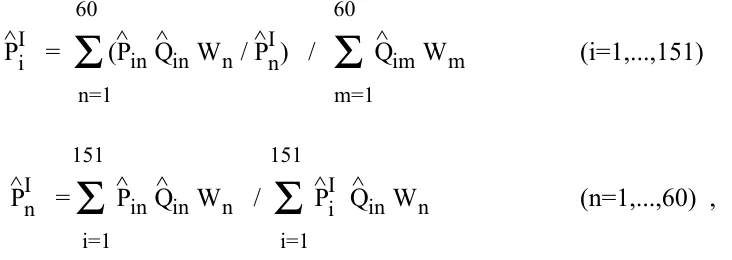
3. Estimates of GDP Based on International and Regional Prices

Table IV.3 of the ICP database, when adjusted for population size, yields expenditures

EI_in = P^I_in Q^_in = P_inI Q_in

for 151 basic headings and 60 countries. The set of average international price ratios

P^I_i = P_iI / _Pi,US

is obtained by solving the set of equations6

P ^I

i =

Σ

n=1 60

(P^_in Q^_in W_n / P^I_n) /

Σ

m=1 60

Q^_im W_m (i=1,...,151)

P^I_n =

Σ

i=1 151

P^_in Q^_in W_n /

Σ

i=1 151

P^I_i Q^_in W_n (n=1,...,60) ,

where all country-specific variables other than P^I_n have been defined in section 2. It follows that

P^I_n = P_nI ,

where

PI_n =

Σ

i=1 151

P_in Q_in /

Σ

i=1 151

PI_i Q_in

6_{Although the equations presented here represent the essence of the ICP calculation, some}

(16)

is the purchasing power parity of the currency of country n. The set of equations is solved for P^I_i (i=1,...,151) and P^I_n (n=1,..,60) for given values of the P^_in , Q^_in and W_n.

This system is an adaptation of the Geary/Khamis system7_{and can be}

interpreted as follows. According to the first set equations, the international price of the ith commodity is the quantity-weighted average of purchasing-power-adjusted prices of the ith commodity in the 60 countries (or, more correctly, supercountries). The second set of equations maintains that the purchasing power of a country's currency is equal to the ratio of the cost of its total bill of goods at national prices to the cost at world prices. One equation in the system is redundant in the sense that it can be derived from the others, and the system is closed by imposing the normalization rule

Σ

i=1 151

P^I_i Q^_i,US =

Σ

i=1 151

P^_i,US Q^_i,US .

Prices derived in this manner have a number of desirable properties including base-country invariance, transitivity, matrix consistency and transactions equality.8

Table 6 contains estimates of GDP valued at world prices and expressed in world currency ($I). It is derived from the expenditures EI_in in much the same way as Table 5 is derived from the expenditures E_in. As all expenditures EI_in are already measured in international dollars, no exchange rate conversion is required in this case.

Just as the adapted Geary/Khamis system can be employed to generate a set of average world prices, it can be applied region by region to generate sets of average regional prices. In particular, for GIOM region m, say, the equations

7_{See Geary (1958) and Khamis (1967, 1970 and 1972).}

(17)

Table 6. Gross Domestic Product, Weighted ICP Data, 1980, International Prices, $I x 107 GIOM Region Expenditure Category 1 NAH 2 LAM 3 LAL 4 WEH 5 WEM 9 JAP 10 ASL 11 OIL 12 AAF 13 SSA Private consumption

(18)

P ^R

i =

Σ

nεN(m)

(P^_in Q^_in / P^R_n) /

Σ

lεN(m)

Q^_i_l (i=1,...,151) P

^R

n =

Σ

i=1 151

P^_in Q^_in /

Σ

i=1 151

P^R_i Q^_in ( nεN(m) )

can be solved to yield the regional prices P^R_i and currency PPPs P^R_n. Here N(m) is the set of sequence numbers for countries belonging to region m. Unlike the system for computing the world prices P^I_i , these equations do not include supercountry weights. Thus, for the regional prices calculated in this study, non-ICP countries within the region are not associated with a particular ICP country. As before, one equation in the system is redundant and the normalization rule

Σ

i=1 151

P^R_i Q^_i,US =

Σ

i=1 151

P^_i,US Q^_i,US

is imposed. Eleven sets of regional prices P^R_i (i=1,...,151) can be computed in this manner, one for each of the eleven GIOM regions which contain at least one ICP country.

When an element E_in of Table IV.1 is divided by the corresponding element

P ^

in of Table IV.2, the quantity Q^in is obtained. Hence a matrix ERin of expenditures based on average regional prices and expressed in regional dollars ($R) can be generated by multiplying the Q^_in by the average price P^R_i of commodity i in the region to which country n belongs. Once the matrix ER_in is assembled, estimates of GDP valued at regional prices can be derived in the usual manner. These estimates are reported in Table 7.

(19)

Table 7. Gross Domestic Product, Weighted ICP Data, 1980, Regional Prices, $R x 107 GIOM Region Expenditure Category 1 NAH 2 LAM 3 LAL 4 WEH 5 WEM 9 JAP 10 ASL 11 OIL 12 AAF 13 SSA Private consumption

(20)

Thus, if the exchange rates between the US, international and regional currencies are taken to be determined by purchasing power parity, the rates are all unity and Tables 5, 6 and 7 are effectively expressed in a common currency.

4. Interpretation and Assessment of the GDP Estimates

In the GIOM, an international commodity balance or market clearing constraint is imposed for each traded commodity. That is, the model does not differentiate between traded commodities of a particular type (e.g., Textile and

apparel) produced in different regions. Hence, for a traded commodity, the model's

database should include estimates of private consumption in each region measured in a common physical unit. This requirement usually presents two kinds of difficulty.

Firstly, even within a region, a GIOM commodity (such as Textiles and apparel) typically represents a collection of unlike items (such as shirts and shoes) which cannot simply be added together. The usual solution is to define the unit of measurement to be the fraction of total consumption of Textiles and apparel in the region in the base period that could have been purchased with one dollar. Thus, the physical unit of Textiles and apparel becomes a bundle of unlike items combined in the same proportions as they were in base period consumption. For a multiregion model, however, there is no presumption that the base period proportions will be the same in each region, or even that the same items will always be represented in the bundles. That is, the physical unit of Textiles and apparel will not generally be the same in all regions. This problem can be alleviated, but not eliminated, by increasing the level of disaggregation employed in the model. Whatever level is finally implemented, residual differences in the composition of the base period bundle across regions will always remain and one can only abstract from their implications.

The other kind of difficulty arises because the relative prices of commodities differ between regions in the base period. Thus, even if the base period bundle of

Textiles and apparel combines its constituent items in the same proportions in all

(21)

embodied in the estimates of Table 5 (which are based on the domestic prices of each country), but not in the estimates of Table 6 (which are base on a common set of world prices).

Table 6, then, shows 1980 expenditures on various commodities measured in world prices and expressed in world currency. But it also shows the physical purchases of those commodities, the physical unit being the amount that could have been purchased for one international dollar in the base period. Thus, for example, the private sector in High-income North America (region NAH) consumed 17460 x 107 units of Textiles and apparel in 1980, more than 22 times the amount (766 x 107) consumed in Sub-Saharan Africa (region SSA). With this convention, the base period international price of a commodity expressed in world currency is always one dollar.

Now, assuming that US currency, world currency and all regional currencies exchange according to purchasing power parity, Table 7 can be interpreted equally well as being expressed in international dollars or in regional dollars. In that case, Table 7 determines the base period regional prices of commodities corresponding to the system of physical units established in Table 6. For example, the regional base period price in world currency of Textiles and apparel in High-income North

America is

15052 / 17460 = 0.86 dollars,

whereas the corresponding price in Sub-Saharan Africa is

541 / 766 == 0.71 dollars.

i.e., the regional prices are similar in the base period.

(22)

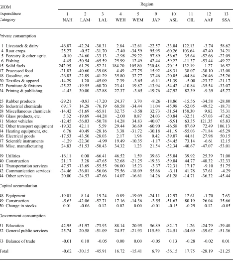
The practical importance of mobilizing the ICP data to determine estimates of private consumption for the GIOM can be guaged from Table 8. This table shows the deviations

D_in = 100 ( E_in -  E_inI  ) /  EI_in

of the absolute values of the expenditures E_in (from Table 5) from the absolute values of the corresponding expenditures EI_in (from Table 6), expressed as percentages of the latter. In other words, the table shows the "errors" that occur when expenditures in physical units are derived via the standard approach (represented by Table 5) rather than the ICP approach (represented by Table 6). The deviations can only be regarded as very large for many expenditure categories.9

Moreover, the pattern of the deviations across categories and across regions is quite erratic. The relevant comparison here is between the magnitudes of the deviations and the magnitudes of the policy (or otherwise) -induced changes in expenditure that models like the GIOM are designed to analyse. Clearly, for many policies of interest, the former magnitudes will often be at least as large as the latter, posing a serious methodological weakness for the standard approach to data preparation.

While expenditures on interregionally traded commodities should be evaluated in terms of a common set of prices in preparing the GIOM database, the same requirement does not hold for commodities that are traded only within a region. For the latter type, the commodity balance constraint is region specific, and the commodity Other services produced and consumed in region NAH, say, is treated as a different commodity to Other services produced and consumed in region SSA. Thus it does not matter whether expenditure in region NAH on Other services is

9_{Note, however, that the deviations are not so large as to be inconsistent with other}

experience from the International Comparison Project. Kravis and Lipsey (1990, p.1), for example, offer the following assessment:

(23)

Table 8. Expenditure Deviations Din , Per Cent GIOM Region Expenditure Category 1 NAH 2 LAM 3 LAL 4 WEH 5 WEM 9 JAP 10 ASL 11 OIL 12 AAF 13 SSA Private consumption

1 Livestock & dairy -46.87 -42.24 -30.31 2.84 -12.61 -22.57 -33.04 122.13 -3.74 58.62 4 Root crops 25.27 -0.57 -31.70 -7.40 -34.59 95.95 -60.26 103.64 47.40 34.21 5 Forestry & other agric. -0.10 -24.60 -33.13 -2.98 -29.22 97.89 -56.62 35.64 -52.66 -22.09 6 Fishing 4.45 -50.54 -65.59 25.99 12.49 42.44 -59.22 -11.37 -53.44 -49.22 15 Solid fuels 242.95 61.29 -52.21 184.20 105.80 230.48 -70.15 132.19 1.27 16.52 17 Processed food -21.83 -40.60 -39.08 4.49 -27.75 15.92 -48.31 38.07 -30.10 -13.08 18 Gasoline, etc. -26.83 -22.89 -41.29 35.80 32.77 37.46 -20.05 -64.84 -26.46 -25.26 20 Textiles & apparel -14.29 1.20 -45.09 7.39 -3.65 -6.11 -51.39 -5.00 -23.37 -21.17 22 Furniture & fixtures -25.22 -19.55 -60.70 23.41 19.87 -13.94 -54.42 -10.84 -35.54 -33.07 24 Printng & publishng -1.43 30.00 -37.88 27.37 -3.65 -19.76 -47.92 82.39 -9.39 45.77 25 Rubber products -29.21 -0.83 -17.20 24.37 3.70 -8.26 -18.86 -15.56 -34.58 -28.80 26 Industrial chemicals 69.17 14.28 -76.19 68.58 -34.44 11.04 -45.98 -52.05 -49.52 -18.71 28 Miscellaneous chemicals -14.42 -51.69 -65.81 32.75 -3.58 32.73 -31.54 158.30 9.82 75.31 30 Glass products, etc. 5.32 -19.69 -44.28 -2.00 0.87 24.03 -50.84 -32.51 -57.03 -47.62 31 Motor vehicles -12.45 -56.03 -50.78 14.28 34.83 -40.07 -5.91 63.35 121.35 65.83 32 Other transport equipment -19.32 42.11 5.59 29.44 36.69 -60.90 -46.58 87.69 72.49 106.13 34 Heating equipment, etc. 6.76 40.49 -28.16 3.38 -31.72 -30.18 -41.19 -55.03 -71.84 -65.29 36 Electrical goods -17.53 -43.50 -28.03 2.17 1.98 0.42 -39.07 44.81 27.98 50.15 37 Scientifc instruments -1.29 -22.36 -4.99 19.49 -10.35 -1.17 -54.45 73.14 -6.61 12.15 38 Misc. manufacturing 24.83 -51.53 -50.43 34.32 1.23 21.54 -52.34 -40.67 -47.07 -53.01 39 Utilities -16.11 0.00 -66.41 46.52 1.59 39.63 -55.04 39.92 25.39 71.00 40 Construction 21.17 3.28 -47.65 32.68 -21.25 -19.33 -59.04 44.77 -48.32 -32.33 41 Transportation services 47.57 -13.69 -55.55 96.00 15.23 -3.37 -72.31 17.17 -9.10 51.75 42 Communication services -24.46 -36.01 -56.06 75.56 -18.09 55.66 -3.11 41.78 37.61 -4.29 44 Other services 20.00 -24.53 -47.66 14.07 -16.61 14.26 -61.28 -14.71 -36.32 -45.44 Capital accumulation

48 Equipment -19.01 8.14 19.24 0.89 -19.09 -24.11 -12.97 12.61 -1.70 7.63 49 Construction -5.63 -42.06 -52.71 17.16 -14.36 -3.55 -51.63 80.19 26.04 35.66 50 Change in stocks 0.01 -0.06 0.12 0.02 0.00 -0.01 -0.15 -0.29 0.12 -0.05 Government consumption

(24)

taken to be 66599 x 107 units with a world price of one dollar and a regional price (in world currency) of

80260 / 66599 = 1.21 dollars,

or to be 80260 x 107 units with a regional price of one dollar and a world price of

66599 / 80260 = 0.83 dollars.

In other words, for commodities that are not traded between regions, private consumption in physical units can be determined equally well from Table 6 or Table 7.

In CGE models, commodities of the same type produced in different regions are generally treated as different commodities whether they are traded between regions or not; i.e., markets generally clear separately for all commodities produced in different regions. Hence there is no requirement that they be measured in common physical units. However, as the CGE approach assumes that agents can always tell the difference between varieties of a commodity such as Textiles and apparel

produced in different regions, it imposes its own formidable reqirements for data in the form of bi-lateral trade flow matrices.

(25)

5. Concluding Remarks

This paper has presented a method for obtaining various estimates of GDP and its components for 1980. The estimates conform as far as possible to the sectoral and regional classifications of the global input-output model (GIOM) of Duchin et al., and are based on three different sets of relative prices: domestic relative prices for 60 ICP countries (Table 5), a set of average world prices (Table 6) and 11 sets of average regional prices (Tables 7).

(26)

References

Burniaux, J-M, F.Delorme, I.Lienert, J.P.Martin and P.Hoeller (1989), "WALRAS - A Multisector, Multicountry Applied General Equilibrium Model for Quantifying the Economy Wide Effects of Agricultural Policies", OECD Economic Studies, 13 (Winter), 69-102.

Deardorf, A.V. and R.M.Stern (1986), The Michigan Model of World Production and Trade, MIT Press, Cambridge, Massachusetts.

Duchin, F., G.Lange and T.Johnsen (1992), "Strategies for Environmentally Sound Development: An Input-Output Analysis", Final Report to the United Nations, Institute of Economic Analysis, New York University, New York.

Duchin, F., G.Lange and T.Johnsen (1994), Ecological Economics, Technological Change and the Future of the Environment (forthcoming).

EUROSTAT (1983), Comparison in Real Values of the Aggregates of ESA, 1980, EUROSTAT, Luxembourg.

Hill, T.P. (1982), Multilateral Measurement of Purchasing Power and Real GDP, EUROSTAT, Luxembourg.

Kravis, I.B., A.Heston and R.Summers (1982), World Product and Income: International Comparisons of Real Gross Product, Johns Hopkins University Press, Baltimore.

Kravis, I.B. and R.E.Lipsey (1990), "The International Comparison Program: Current Status and Problems", Working Paper No.3304, National Bureau of Economic Research, Cambridge, Mass.

Leontief, W., A.Carter and P.Petri (1977), The Future of the World Economy, Oxford University Press, New York.

Mercenier, J. and J.L.Waelbroeck (1986), "Effect of a 50 per cent Cut in the Varuna Model", in T.N.Srinivasan and J.Whalley (eds.), General Equilibrium Trade Policy Modelling, MIT Press, Cambridge, Massachusetts.

Meagher, G.A. (1991), "The International Comparison Project as a Source of Data for a Global Input-Output Model", Working Paper No.01-91, Institute for Economic Analysis, New York University, New York.

United Nations (1971a), Indexes to the International Standard Industrial Classification of All Economic Activities, Statistical Papers, Series M, No.4, Rev.2, Add.1, United Nations, New York.

United Nations (1971b), Recommendations for the 1973 World Programme of Industrial Statistics, Part II: List of Selected Products and Materials, Statistical Papers, Series M, No.54 (Part II), United Nations, New York.

United Nations (1986), World Comparisons of Purchasing Power and Real Product for 1980, Phase IV of the International Comparison Project, Part One: Summary Results for 60 Countries, United Nations, New York.

United Nations (1987), World Comparisons of Purchasing Power and Real Product for 1980, Phase IV of the International Comparison Project, Part Two: Detailed Results for 60 Countries, United Nations, New York.

(27)