Comparison of the innovative method for linear
viscoelasticity problems with standard ansys
tools using simple tasks
Mikhail Pavlov1,*, Aleksander Svetashkov1 , and Vladimir Barashkov2
1Tomsk Polytechnic University, 634050 Tomsk, Russia
2Tomsk State University of Architecture and Building , 634003 Tomsk, Russia
Abstract. A description of the original method for solving problems of linear viscoelasticity, based on the separation of spatial and temporal variables and the reduction of this problem to an elastic problem, is presented in the paper. We compared the solutions given by this method, as well as those obtained using standard ANSYS tools, with known analytical solutions. The results show the effectiveness of the new method.
1 Introduction
A large number of works devoted to the inclusion of the viscoelastic properties of structural materials, including some informative monographs [1–7] and others, exist. At the same time, despite the substantial theoretical study of the issue, the number of problems for which an exact analytical solution was obtained remains small. This is primarily due to the high complexity of such tasks. Moreover, most applied problems of the linear theory of elasticity also do not have an exact analytical solution. For viscoelastic problems, a number of approximate methods have been developed; methods based on the Laplace transform [6, 8] are the most well-known. On the other hand, advances in computing have made it preferable to use discrete numerical methods for both linear elasticity problems and various non-linear problems, including consideration for viscoelastic properties. At the same time, the development of new numerical algorithms and even the use of existing ones are associated with a large amount of work on writing and debugging the program code implementing one or another algorithm for solving the problem. In this regard, in practical work, specialized software systems, such as ANSYS, Nastran, ABAQUS (commercial), Elmer, CalculiX (freely distributed), etc., have become very common. As a rule, the following approach is applied to solving the problems of viscoelasticity in such software. The properties of a viscoelastic material are determined by using the functions of bulk and shear creep, represented in the form of line segments Prony’s ranks (the sum of exponents). The viscoelastic solution is obtained by integrating the elastic solution obtained for the initial moment of time. Specific computational algorithms may differ, but in the most common systems, integration is replaced by calculation using recurrent formulas, for which a step must be set by time [9-11]. The substantiation of some such formulas is contained in
[12-14]. The universality of this approach is its advantage; however, the accuracy of the solutions obtained with its help directly depends on the size of the time step, and, accordingly, the computing resources spent. Methods for solving problems of viscoelasticity that are convenient for use in conjunction with existing engineering analysis software also exist besides those indicated. These are the methods having a replacement, a viscoelastic problem for an elastic one, whose solution (stresses, strains, displacements) is equivalent to solving the original problem. Such methods are described, for example, in [15-22]. This type of method developed by the authors is used in this work. Demonstration of the advantages of this method by comparing the solutions given by them and standard ANSYS tools with analytical solutions of the simplest problems is the goal of the work.
2 Problem description
When writing equations, we will use the generally accepted position of summation over repeated indices. A comma in the indices of any value means differentiation by the variable indicated after the comma. The physical relationships for a linear-viscoelastic body are written as
* 2 * 2 * 3
ij K G ij G ij
, (1)
where σij – stress tensor components, εij – deformation tensor components, indexes i, j –
take values from1 to 3, θ = εijδij – volumetric deformation, K*, G* – operators of bulk and
shear relaxation.
* 0 0 t KK K t d
, (2)
* 0
0
t
ij ij G
G G t d
. (3)
In its turn, ΠK, ΠG – are the nuclei of the operators of volume and shear relaxation,
respectively, t – the time counted from the initial moment for the problem being solved. Equilibrium equations in displacements for a linear-viscoelastic body in the absence of mass forces have the form
* 2 * θ, * θ, 0
3 i i i
K G G u
, (4)
where ui – components of displacement, Δ – Laplace operator.
0
1, 2, 3, 1, 2, 3 , 1, 2, ,
i im im
u x x x t u x x x H t m n , (7)
Γ1 – section of the border, where loads are set, Γ 2 – section of the border, where
displacements are set. In its turn, Sik0, uim0 – components of boundary loads and
displacements, depending only on spatial variables, Hik, Him – some time functions.
Using the analytical method of separation of variables, instead of the boundary problem of the linear theory of viscoelasticity defined by (1), (4), (5), we solve the boundary problem of the theory of elasticity with the governing equations
0 2
2 3
ij k tc g tc ij g tc ij
. (8)
Equilibrium equations in displacements
2
, , 0
3
c c i c i i
k t g t g t u
. (9)
In the transition to the linear elasticity problem, the boundary conditions (5) remain unchanged. Here
* 1 ,
* 1c c
H H
k t g t
K H GH
, (10)
where H, is one of the functions of time included in (6), (7), K*-1, G*-1 – inverse K* and G*
operators.
The justification of the analytical calculations used in the formulation of relations for
kc(t), gc(t), is not given here due to the limited scope of the publication.
2 Comparison of solutions obtained by different methods
To illustrate the effectiveness of the method under discussion, we consider solutions to a number of model problems. We compare the results of the solutions with the well-known analytical solutions, as well as with the solutions obtained using the ANSYS software package of applied finite element analysis. The choice of a particular package is connected, firstly, with its dominant position in the field of engineering calculations, and, secondly, with the availability of a convenient tool for defining user functions — the internal programming language APDL (ANSYS Parametric Design Language).
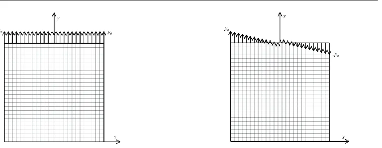
As a simple example, we consider the problem of stretching and bending a viscoelastic plate. For each of the problems, the finite element model, which is used to obtain the elastic solution in the framework of the new method, as well as to solve the viscoelastic problem using standard ANSYS tools, has been prepared.
Fig. 1. Finite element meshes and loading schemes
The mechanical properties of the plate are determined by setting the operators G*, and
K*. For ease of obtaining an analytical solution, we set the volume properties to be constant.
* 0
K H K H, (11)
where K0 – bulk modulus. The kernel of operator of shear relaxation we assume an
exponential
* 0
0
t t
G HG H t e H d
, (12)where G0 –instantaneous value of shear modulus, λ, γ –kernel parameters. The choice of the
type of kernel is determined, on the one hand, by considerations of simplicity of calculations, and, on the other hand, by the fact that in the most common software engineering analysis complexes the viscoelastic properties of materials are set by using line segments of Prony’s series (sum of exponentials).
In the case of uniaxial stretching, the plate works like a rod. The expression that determines the elongation of a viscoelastic rod, in this case has the form [23]
* 1 0 F
u yE
A
. (13)
where y – section coordinate (in accordance with the coordinate system shown in Fig.1),
u – section displacement, F0 – constant component of tensile load, A – cross sectional area,
E* – relaxation operator.
Under the action of the load corresponding to right side Fig.1, the plate is in a state of pure bending. The bending moment M0 is related to the value F0 by the ratio
2
0 0
6
l
where J – the beam moment of inertia. In this case
* 1
0 0 0
1
3 9
t
t H t
E H H t e H d
G K
. (16)For the numerical implementation, the values of the model parameters presented in
Table 1 are taken.
Table 1. The numerical model parameters
Parameter Value
Plate dimensions 1×1 m
Instantaneous shear modulus G0 6·108 Pa;
bulk modulus K0 14·108 Pa
Kernel parameter λ 0,2
Kernel parameter γ 0,01
Load intensity F0 1 N/m
Since analytical solutions (13), (15) are obtained using creep kernels, and when setting the viscoelastic properties of a material in ANSYS, creep functions are used, it is necessary to ensure the correspondence of these functions and kernels. For the case of a non-relaxing volume, such a correspondence exists when the shear relaxation function contains only one term, and the following relations hold
1 1
G
, (17)
1
G
. (18)
Here τ1G, α1G – shear relaxation function parameters specified in ANSYS.
To eliminate the influence of edge effects, a comparison of the results of numerical calculations was carried out for the central node of the finite element mesh.
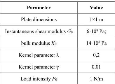
Fig. 2. The relative discrepancy of solutions of the problem of stretching, obtained by different methods with respect to the analytical method
Fig. 3. The relative discrepancy of solutions of the problem of bending, obtained by different methods
with respect to the analytical method
As can be seen from Fig.2, Fig.3 the error given by standard means can already reach 7 % in the simplest case, while the error of the new method is about 10-10 %, which is
practically zero.
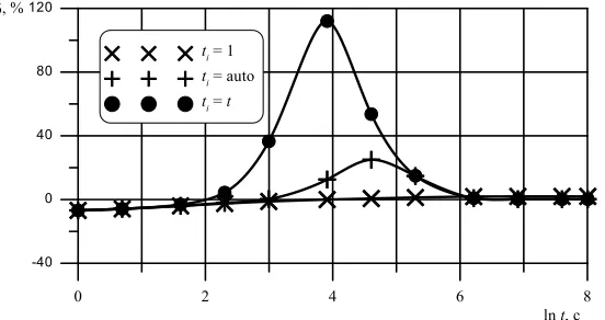
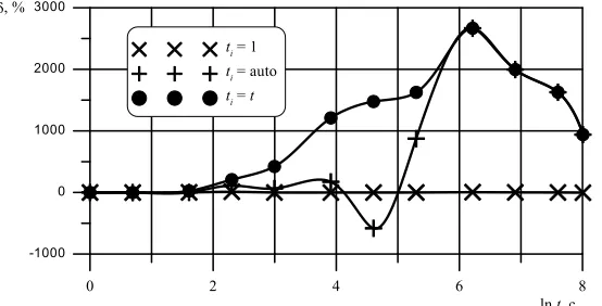
As already mentioned, when using standard ANSYS tools, the accuracy of the solution obtained depends on the choice of the time step ti, used to integrate the elastic solution. The
accuracy comparison for the three cases is shown in Fig. 4, Fig. 5: 1) step ti is equal to 1 s,
Fig. 4. The errors of solutions to the stretching problem obtained by different methods with respect to the analytical method for different integration steps
Fig. 5. The errors of solutions to the bending problem obtained by different methods with respect to
the analytical method for different integration steps
Fig. 6. CPU time for different steps of integration and using the new method
As can be seen from Fig.2 – Fig.5 for the case of quasistatic loading as t → ∞, the accuracy given by standard ANSYS tools increases. The results of the comparison of the errors of the problem of stretching the plate for the case of a load variation according to the harmonic law (H(t) = sin t) are shown in Fig.7 – Fig.8. For the task of bending, the graphics have a similar appearance.
Fig. 7. Relative discrepancy between solutions of the stretching problem obtained by different
The results cited in Fig.7 – Fig.8 show that with more complex than quasi-static loading, choosing too large an integration step using standard ANSYS tools can lead to completely unreliable solution results, especially for tasks with large time intervals. In its turn, the accuracy and resource intensity of the method proposed by the authors does not depend on the length of the time interval.
3 Conclusion
The comparisons made suggest that the approach developed by the authors for solving problems of viscoelasticity has the following advantages. Firstly, it is ease of use compared with the methods based on the Laplace transform and the Volterra method. Secondly, the accuracy of the new method does not depend on the computing resources used, which is an advantage relative to the algorithms for integrating the elastic solution using recurrent formulas.
References
1. J. D. Ferry, Viscoelastic properties of polymers (Wiley, 1980)
2. S. Doubal. J. Doubal, Theory of viscoelasticity handbook (Delter, 2014)
3. A. D. Drozdov, Mechanics of Viscoelastic Solids (Wiley, 1998)
4. F. Mainardi, Fractional Calculus and Waves in Linear Viscoelasticity (Imperial College Press, 2010)
5. Y. N. Rabotnov (in Russian – Elementi nasledstvennoi teorii mechaniki tverdih tel) (Nauka, 1977)
6. A. A. Il’iushin, B. E. Pobedrya (in Russian – Osnovi matematicheskoy teorii termovyazkouprugosti) (Nauka, 1970)
7. M. A. Koltunov, V. P. Mayboroda, V. G. Zubchaninov (in Russian – Prochnostnie rascheti izdelyi iz polymernih materialov), (Mashinostroenie, Moskow, 1983)
8. Schapery R. A. Journal of Composite Materials. 1(3). 228-267, (1967)
9. ANSYS Mechanical APDL Theory Reference (ANSYS Inc, 2013)
10. Simcenter Nastran 2019.2 Advanced Nonlinear Theory and Modeling Guide (Siemens Product Lifecycle Management Software Inc., 2019)
11. ABAQUS Theory Manual (Dassault Systems, 2019)
12. R. L. Taylor, K. S. Pister, G. L. Goudreas, International Journal for Numerical Methods in Engineering. 2, 45-59, (1970)
13. J. C. Simo, Computer Methods In Applied Mechanics and Engineering, 60, (2). 153-173, (1987)
14. G. A. Holzapfel, Nonlinear Solid Mechanics. A Continuum Approach for Engineering (Wiley, 2001)
15. A. A. Adamov, V. P. Matveenko, N. A. Trufanov, [et. al.] (In Russian – Metodi prikladnoy vyazkouprugosti). (UrO RAN, 2003)
16. V. V. Moskvitin, (In Russian – Soprotivlenie vyazko-uprugih materialov primenitelno k zaryadam raketnih dvigateley na tverdom toplive) (Nauka, 1972)
17. A. Svetashkov, N. Kupriyanov, K. Manabaev, Acta Mechanica, 229, (6), 2539-2559, (2018)
19. A. A. Svetashkov [et al.] Key Engineering Materials : Scientific Journal. High Technology: Research and Applications (HTRA 2016), 743, 217-222, (2017)
20. A. A. Svetashkov, A. A. Vakurov, IOP Conference Series: Materials Science and Engineering. Mechanical Engineering, Automation and Control Systems (MEACS2015), 124, 012099 (2016)
21. A. A. Svetashkov, Mechanics of Composite Materials, 36, (1), 37-44, (2000) 22. A. A. Svetashkov, S. M. Pavlov, Russian Physics Journal, 36, (4), 400-406, (1993)