Energy Taxes and Greenhouse Gas Emissions in Australia

Full text

(1)CENTRE of POLICY STUDIESand the IMPACT PROJECT. Eleventh Floor Menzies Building Monash University Wellington Road CLAYTON Vic 3800 AUSTRALIA Telephone: (03) 9905 2398, (03) 9905 5112. from overseas: 61 3 9905 2398 61 3 9905 5112. Fax number: (03) 9905 2426 e-mail Web site:. 61 3 9905 5486 impact@vaxc.cc.monash.edu.au http://www.monash.edu.au/policy. Energy Taxes and Greenhouse Gas Emissions in Australia by. R. A. McDOUGALL Centre of Policy Studies Monash University. General Paper No. G-104 December 1993. Reprinted December 1999 ISSN 1031 9034. ISBN 0 642 10345 3. The Centre of Policy Studies (COPS) is a research centre at Monash University devoted to quantitative analysis of issues relevant to Australian economic policy. The views expressed herein do not necessarily represent those of any sponsor or government..

(2) ABSTRACT. A feature of recent policy discussion both in Australia and overseas has been a heightened interest in energy taxes and fuel taxes of various kinds. These taxes have been advocated on various grounds, notably their role in discouraging greenhouse gas emissions. At the same time, at least in Australia, greenhouse policy discussion has been redirected more towards small-scale sector-specific interventions, and away from economy-wide measures such as a carbon tax. In this context it becomes of interest to ask, how effective might an energy tax be in reducing carbon emissions? Here we use the term energy tax to mean fossil fuel taxes excluding carbon taxes. A carbon tax is levied on carbon dioxide emissions or some closely related basis, while an energy tax is levied on some other basis such as energy content. The paper presents simulation results designed to address these questions. The simulations are performed using the ORANI model of the Australian economy, in a version containing several energy-specific enhancements. These include greater detail on energy production and use in the database, and a wider range of substitution possibilities in energy production and use in the theoretical structure. The database enhancements include extensive disaggregation of the two largest parts of the energy sector, fossil fuels and electricity. The theoretical developments cover substitution between energy and capital, between different sources of energy, between different techniques of generating electricity, and between different modes of transport. We find that a broad-based energy tax would be comparable in effectiveness to a carbon tax in reducing greenhouse gas emissions. This is because like the carbon tax it would bear heavily on the cheaper fossil fuels and would induce emission abatement through fuel switching. Taxes such as a petroleum products tax which excluded the cheaper fossil fuels would be much less effective.. i.

(3) Contents Abstract. i. 1.. Background. 2. 2.. Model. 3. 2.1 Enhancements for long-run comparative statics. 4. 2.2 Enhancements for energy sector analysis. 7. 3.. Simulations. 10. 4.. Conclusions. 18. References. 19. Appendix 1:. Changes to the ORANI theoretical structure for ORANI-E. 21. Appendix 2:. Database changes for ORANI-E. 33. ii.

(4) Tables and Figures Table 1:. Ad valorem tax rates on fossil fuels. 12. Table 2:. Estimated effects of energy, carbon and petroleum products taxes on fossil fuel energy use and carbon dioxide emissions. 13. Estimated effects of energy, carbon and petroleum products taxes on selected macro variables. 13. Estimated effects of energy, carbon and petroleum products taxes on activity, by broad sector. 15. Estimated effects of energy, carbon and petroleum products taxes on activity in selected industries. 16. Estimated effects of energy, carbon and petroleum products taxes on employment, by occupation. 17. Table A2.1:. Mineral supply elasticities. 33. Table A2.2:. Emission intensities. 33. Table A2.3:. Electricity supply: cost summary, by disaggregated industry. 34. Electricity supply: fuel use summary, by disaggregated industry. 34. Table 3: Table 4: Table 5: Table 6:. Table A2.4:. Figure 1:. Nesting structure for energy end use. 9. Figure 2:. Nesting structure for electricity supply. 10. iii.

(5) ENERGY TAXES AND GREENHOUSE GAS EMISSIONS IN AUSTRALIA1 by R.A. McDougall A feature of recent policy discussion both in Australia and overseas has been a heightened interest in energy taxes and fuel taxes of various kinds. These taxes have been advocated on various grounds, but one argument commonly put for them is their supposed greenhouse friendliness. At the same time discussion in Australia on policy aimed specifically at greenhouse objectives has tended to focus more on small-scale sector-specific interventions, and less on economy-wide measures such as a carbon tax. Our focus in this paper is on the greenhouse effects of energy taxes. More specifically we are concerned with taxes levied on fossil fuels but calculated on some different basis than carbon content. A typical example is a tax on the energy content of fossil fuels. We aim to address a number of questions raised by current policy discussion. For one, when energy taxes are advocated as greenhouse-friendly measures, how greenhousefriendly in fact are they? In particular, how do they compare with a measure aimed specifically at greenhouse abatement, namely the carbon tax? Another question is how energy and carbon taxes differ in their non-greenhouse effects. Where greenhouse abatement is acknowledged as a policy goal but carbon taxes are not adopted, the reason may be that the non-greenhouse effects of the carbon tax are considered unacceptable. Such effects might include economy-wide welfare losses or severe adjustments to individual economic sectors. Are the non-greenhouse effects of an energy tax likely to prove more acceptable than those of a carbon tax? This paper uses a computable general equilibrium model to address these questions. The model is ORANI, a widely used model of the Australian economy, in a version extended for use in long-run energy policy analysis. With it we simulate several energy-related tax options Ñ a carbon tax, an energy tax covering all fossil fuels, and a tax restricted to refined petroleum products. 1. The research reported in this paper has been undertaken by the Centre of Policy Studies, as part of the MONASH project and the joint ABARE-CoPS project for system-wide analysis of least cost combinations of options to reduce greenhouse gas emissions. The MONASH project has been undertaken with financial assistance from the Commonwealth Government, through the Industry Commission. The greenhouse gas project has been undertaken with financial assistance from the Commonwealth Department of the Environment, Sport, and Territories, and the Victorian Environmental Protection Agency.. 1.

(6) Section 1 contains a brief qualitative discussion of energy taxes and greenhouse emissions. Section 2 describes ORANI model enhancements used in this study. Section 3 describes the design of the simulations and reports the simulation results, and the section 4 summarises and concludes.. 1. Background Energy taxes have recently gained favour with some governments and interest groups. The Clinton administration in the United States of America has proposed (unsuccessfully) a Ômodified Btu taxÕ; the Australian government has increased petrol excise; and the EC Commission has proposed a mixed energy-cum-carbon tax (Energy Economist May 1993 pp. 6-10, Dawkins and Willis 1993, Nicoletti and OlivieraMartins 1992). Various parties have given various reasons for raising energy taxes. The Australian Government has cited revenue raising and energy conservation in support of its petroleum excise increases, while press commentary has referred to greenhouse benefits (e.g. Wallace 1993). The US Department of Energy has cited revenue raising, reductions in greenhouse emissions, and reduced reliance on fuel imports in support of a Btu tax. The EC CommissionÕs plan was developed as part of a strategy for stabilising greenhouse emissions. In Australia and the USA the motive for the tax is fiscal, with environmental considerations affecting the choice of fossil fuels as a tax base. In the EC the stated motive is environmental, with non-environmental considerations perhaps influencing the choice of a combined carbon-energy tax rather than a straight carbon tax. At the same time in Australia support for a carbon tax appears to have waned. The National Greenhouse Response Strategy (Commonwealth of Australia 1992) favours information collection and narrowly focused Ôno-regretsÕ options over economy-wide measures. Of options for stronger greenhouse action those with greatest current political currency are perhaps subsidies for research into renewable energy technologies. Some non-economists concerned with environmental policy appear to regard the carbon tax instrument as blunt, crude and costly. Many economists on the other hand have promoted the carbon tax as a well targeted feasible instrument for greenhouse emission abatement (e.g. Pearce 1991). It is not an ideal instrument: it excludes greenhouse gases other than carbon dioxide, and sources and sinks of atmospheric carbon dioxide other than fossil fuel combustion. These exclusions however would facilitate its practical implementation while still leaving it better targeted against greenhouse emissions than an energy tax. A carbon tax would be better targeted against carbon dioxide emissions than an energy tax because it would discriminate better between fossil fuels. The ratio of carbon. 2.

(7) dioxide emissions to energy content (emission coefficient) varies across fuels, with coal having a higher emission coefficient and oil and gas lower coefficients. So compared to an energy tax, a carbon tax would fall relatively more heavily on coal and more lightly on oil and gas (table 1). Taxes on fossil fuels could reduce greenhouse emissions in several ways. They could reduce the overall level of economic activity. They could induce shifts in consumption from more energy-intensive to less energy-intensive products, and shifts in production from more energy-intensive to less energy-intensive processes. And they could induce fuel switching from more highly taxed to less highly taxed fuels. Carbon and energy taxes would differ in their fuel switching effects. Both kinds of tax would induce some switching, since both would increase coal prices relative to oil and gas. But since a carbon tax would change relative prices more, it would induce more switching than an energy tax. Previous studies suggest that fuel switching would be a major source of greenhouse abatement with a carbon tax. For instance a report by the ABARE for the Ecologically Sustainable Development Working Groups found that Ôthe most cost effective way to make large carbon dioxide emission reductions is by changing the fuel mix used in electricity generationÕ (Jones, Naughten, Peng and Watts 1991 p. 28). An energy tax would be less effective than a carbon tax in bringing about such a change. We expect then that an energy tax would be less effective than a carbon tax in reducing greenhouse gas emissions. Whether the difference in effectiveness would be great or trivial is less clear. Also less clear is the extent to which the sectoral and macroeconomic impacts of an energy tax would differ from those of a carbon tax. To answer these questions we need a quantitative analytical framework with both economy-wide coverage and energy-sector detail. Such a framework is provided by the extended ORANI model described in the following section.. 2. Model The vehicle for the analysis in this paper is ORANI-E, a general equilibrium model of the Australian economy incorporating a detailed representation of the Australian energy sector. ORANI-E is a version of the well-known ORANI model used widely in academia, government and business for Australian economic policy analysis (Dixon, Sutton, Parmenter and Vincent 1982, Powell and Snape 1993). Besides the standard ORANI structure, ORANI-E contains enhancements designed to support long-run comparative static analysis of energy-related issues. The model is implemented using the GEMPACK suite of model development software (Harrison and Pearson 1993a). We write down the theoretical structure in close-to-. 3.

(8) ordinary algebraic notation; we then use the GEMPACK program TABLO to translate this into FORTRAN code (Harrison and Pearson 1993b). Like standard ORANI, ORANI-E exhibits the neoclassical dichotomy between the price level on the one hand and relative prices and real activity on the other. At least one price must be set exogenously; if just one price is exogenous, it acts as numeraire. ORANI-E can be run in either comparative static or forecasting mode. For forecasting simulations it uses theoretical structure inherited from another version of the model, ORANI-F (Horridge, Parmenter and Pearson 1993). In forecasting mode the model results represent changes in economic variables through time. In comparative static mode they represent differences between a base case state and an alternative state of the economy at a given point in time. In comparative static mode, differences between the base case and the alternative state arise from different values applied to exogenous economic variables. The exogenous variables refer to values over some simulation period, and the endogenous variables to values at the end of the period. Thus the endogenous variables represent the response of the economy after some passage of time to the external shocks represented by the exogenous variables. By specifying which variables should be exogenous and which endogenous, a user of the model can tailor an economic environment to either a short or a long simulation period. So for instance in a short-run simulation industry capital stocks might be fixed exogenously, while for a long-run simulation rates of return might be fixed and capital stocks allowed to adjust to external shocks. To support long-run comparative static analysis ORANI-E contains extensive enhancements centered around the household and government sector budget constraints. These enhancements allow the aggregate capital stock to expand in response to changes in economic conditions but require the expansion to be financed by increased domestic saving or foreign capital inflow. Increases in foreign capital inflow lead over time to increases in net income payments abroad. Section 2.1 describes enhancements in ORANI-E designed to adapt it to long-run comparative static analysis. Section 2.2 describes energy-related enhancements. TABLO source code for modifications to the theoretical structure is provided in Appendix 1. 2.1. Enhancements for long-run comparative statics In this section we describe modifications to the model designed to adapt it to long-run comparative static analysis. These modifications include a long-run treatment of investment, a government budget constraint, accounting for liabilities incurred in expanding the national capital stock, the introduction of a consumption function, and. 4.

(9) use of after-tax rates of return on assets used in production. We also modify the database to recognize resource availability constraints on mining supply. Earlier versions of ORANI adapted to long-run comparative static analysis include the ÔHorridge closureÕ (Horridge 1985) and FH-ORANI (Dee 1989). ORANI-E borrows extensively from these, simplifying in some areas and elaborating in others. Investment ORANI-E inherits from standard ORANI a vector variable representing investment flows in each industry. In comparative static mode this variable refers to investment at the end of the simulation period. Following Horridge (1985) we require the rate of investment at the end of the simulation period to be proportional to the size of the capital stock at the end of the period. With this treatment the rate of growth in the capital stock at the end of the simulation period is not affected by shocks to the model, but conforms to some long-run trend. Shocks to the model do however affect the size of the capital stock at the end of the simulation period and the implied rate of growth in the capital stock through the period. Budget constraint We introduce into the model variables representing an average income tax rate, income tax revenue, and a measure of government budget imbalance. This enables us to impose in long run simulations a government budget constraint making the budget imbalance variable exogenous and the income tax rate endogenous. Liabilities incurred in expanding the national capital stock We recognize in ORANI-E not only the industry fixed capital stocks recognized in the standard model but also several other asset types. These are industry stocks of working capital, industry stocks of land, and household net debt. To explain the composition of household wealth would require the implementation of finance theory concepts involving a radical revision to the theoretical structure. For the present paper we provide instead a highly simplified treatment using strong simplifying assumptions. We treat the household sector as the owner of all capital and land employed in Australia. We assume that the only other item on the household sector balance sheet is household net debt. Then given capital and land values and household net wealth, we can determine household net debt as a residual. Capital and land values are determined elsewhere in the model consistently with asset rentals and rate of return relations described below. Household net wealth is determined by an accumulation equation (following McDougall 1993a) taking account of household saving levels through the simulation period.. 5.

(10) This treatment ensures that changes in stocks of domestic physical assets must be financed either from household sector savings or by incurring external debt. Consumption We introduce into the model a simple consumption function expressing consumption expenditure as the product of household disposable income and an average propensity to consume. Household disposable income is equal to household income times one minus the income tax rate. Household income is equal to factor income less net interest payments, and factor income is equal to the sum of income from labour, fixed capital, working capital, and land. Household net interest payments are equal to the product of household net debt and the pre-tax rate of interest. After-tax rates of return Physical asset rentals and asset values are related by pre-tax rates of return. Pre-tax rates of return depend on after-tax rates of return and the income tax rate. In long-run asset market equilibrium the after-tax rate of return on each industryÕs physical assets is equal to to the after-tax rate of interest on household debt plus a risk premium. The after-tax rate of interest on household debt depends on the pre-tax interest rate and the income tax rate. The pre-tax interest rate is exogenous; we think of it as determined by an international interest parity condition. Fixed factor usage in mining We modify the database to recognize resource availability constraints on mineral supply. The modifications include a change in the treatment of mineral royalty payments and changes to factor substitution parameters in mining. Whereas the standard database includes mineral royalty payments in returns to capital, ORANI-E treats them as returns to land. With land a fixed factor in the long-run economic environment, this ensures that even in long-run simulations the supply of minerals is less than perfectly elastic. For mining as for other industries supply elasticities are not set explicitly in the database but depend on land shares in total costs and on factor substitution parameters (Dixon et al. 1982 p. 309). With standard settings for these parameters we obtain longrun mineral supply elasticities higher than for broad-acre agriculture but still appreciably less than infinite (Appendix 2 Table A2.1). 2.2. Enhancements for energy sector analysis In this section we describe enhancements in ORANI-E designed to support energy policy analysis. These modifications include provision for carbon and energy taxation,. 6.

(11) a more flexible theoretical structure for production, disaggregation of the fossil fuel and electricity sectors, and intermodal substitution in freight transport. Carbon taxation We introduce into the theoretical structure provision for taxes on emissions or other ÔbadsÕ associated with domestic usage of both commodities. These taxes are incorporated into the ad valorem commodity taxes included in the standard model; their contribution to ad valorem commodity tax rates depends on intensity coefficients measuring the ratio of bads content to market value for each commodity, and release coefficients measuring the completeness of release of the bads content in each type of usage. In the ORANI-E database used in this paper bads include carbon dioxide, fossil fuel energy content, and petroleum products energy content. This facilitates the modelling of carbon, fuel, and petroleum products taxes. Fossil fuels The commodity group Ôoil, gas and brown coalÕ in standard ORANI is disaggregated into six new commodities (Adams and Dixon 1992): Ñ crude oil, Ñ natural gas, Ñ liquefied petroleum gas, natural Ñ brown coal (lignite), Ñ brown coal (briquettes), and Ñ oil, gas, and brown coal not elsewhere classified. Electricity We disaggregate the electricity industry into seven new industries. Six of these represent electricity generation technologies, and the seventh represents end-use electricity supply. The electricity generation technologies are: Ñ steam turbine, Ñ hydroelectricity, Ñ gas turbine, Ñ combined cycle, Ñ other fuel burning, and Ñ other non-fuel-burning.. 7.

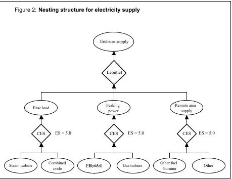
(12) In the database, reflecting conditions in the reference year 1986-87, the first four of these technologies are dominant. Data for the Ôother fuel burningÕ technology derive from existing internal combustion plant; data for Ôother non-fuel-burningÕ from existing wave power plant. We adjust the cost structure of the hydroelectricity industry to take account of supply constraints imposed by the scarcity of suitable unexploited sites for hydroelectricity generation. The method is similar that described above for the mining industry. We reassign some of the industryÕs costs from capital to land, and set the factor substitution parameters to ensure that the elasticity of supply of hydroelectricity is low. The electricity supply industry takes the output supplied by the various generation technologies and transmits and distributes it to end users. A summary of the electricity disaggregation is provided in Appendix 2. Flexibly nested production functions Following McDougall (1993b) we use a flexible nesting scheme for industry production functions. This greatly facilitates the introduction of substitution possibilities not included in standard ORANI. With the ORANI-E database in this paper we use the flexible nesting facility to model energy-capital substitution, inter-fuel substitution, and substitution between different electricity generation technologies. We divide the electricity generation technologies into three groups Ñ base load, peaking power, and remote area Ñ and allow for substitution within each group. The base load technologies are steam turbine and combined cycle, the peaking power technologies hydroelectricity and gas turbine, and the remote area technologies Ôother fuel burningÕ and Ôother non-fuel-burningÕ. Figure 1 shows the nesting structure for energy end use, and Figure 2 the structure for electricity supply. The nesting structure and the substitution elasticity settings follow the ORANI-Greenhouse model (Industry Commission 1991 Appendix G). The settings are 1.2 for the inter-fuel substitution elasticity, 0.5 for energy-capital substitution, and 0.8 for substitution between the energy-capital bundle and labour. For the substitution between electricity generation technologies we set a substitution elasticity of 5.0 within each group.. 8.

(13) Figure 1: Nesting structure for energy end use. Activity level. Leontief. Non-energy commodity 1. Factor-energy bundle. CES. CES. CES. Capital-energy bundle. CES. Capital. Capital-land bundle. Labour type M. CES. Other costs. ES various. Domestic product. ES = 0.35. Labour type 1. g c M ES. Non-energy commodity g - c. ES = 0.8. Labour. ES = 0.0. Energy carrier 1. Number of commodities Number of energy carriers Number of occupations Elasticity of substitution. 9. ES = 0.5. Energy. CES. ES = 1.28. Land. Imports. ES = 1.2. Energy carrier c.

(14) Figure 2: Nesting structure for electricity supply. End-use supply. Leontief. Peaking power. Base load. CES. Steam turbine. ES. ES = 5.0. Combined cycle. CES. Hydro ES = 5.0. Remote area supply. ES = 5.0. Gas turbine. CES. Other fuel burning. ES = 5.0. Other. Elasticity of substitution. Intermodal substitution We introduce intermodal substitution in margin usage of transport services. This allows the assignment of freight transport tasks between road, rail, sea and air transport to respond to relative freight costs. Intermodal substitution elasticity settings follow ORANI-Greenhouse; the elasticities are set at 2.0 for most commodities, but at lower numbers or zero where government regulation reserves some freight tasks for selected transport modes (Industry Commission 1991).. 3. Simulations The main simulation represents the introduction of an energy tax. The tax is levied on fossil fuels, on consumption rather than production (so that imported fuels are taxed, and exported fuels exempted), on the basis of the energy content of the fuels. The tax rate is set so as to collect revenue equivalent to 0.5 per cent of base-case GDP (in. 10.

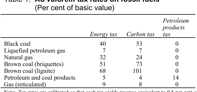
(15) current terms, about two billion dollars). The tax rate in current terms is around 70 cents per gigajoule. For comparison we also present results for two alternative energy-related taxes: a carbon tax and a tax on petroleum products. To assist comparison, each tax has been set so as to collect the same revenue as the energy tax, i.e. 0.5 per cent of base-case GDP. The tax rates are equivalent to around $10 per tonne of carbon dioxide for the carbon tax, and 14 per cent of basic value for the petroleum products tax. The petroleum products tax simulated here differs from the petroleum excise increases in the 1993-94 budget not only in representing a somewhat higher revenue collection but also in applying uniformly to all refined petroleum products. Accordingly the petroleum products tax simulation results are not necessarily indicative of the 1993-94 budget measure. We run the model in comparative static mode in a long-run economic environment. Features of the environment include: Ñ a fixed average propensity to consume out of household disposable income, Ñ a fixed proportion between real government consumption and real aggregate household consumption, Ñ a government budget constraint, met by adjusting the income tax rate, Ñ fixed labour employment, with flexible adjustment of wage rates, and Ñ fixed after-tax rates of return on fixed capital, working capital and land in each industry, with flexible adjustment of fixed capital stocks, working capital rental rates, and land prices, and Ñ a fixed nominal exchange rate serving as numeraire for the price system. The energy and carbon taxes do not affect all fuels equally, but bear most heavily on those fuels which are cheapest relative to their energy or carbon content. Tax rates expressed with respect to physical (energy or carbon) units are converted to a d valorem tax rates using emission intensities showing energy or carbon content per dollar of fuel. The cheapest fuels have the highest emission intensities and the highest ad valorem tax rates. Table 1 shows the ad valorem tax rates applied in the simulations. The underlying emission intensities may be found in Table A2.2 of Appendix 2.. 11.

(16) Table 1: Ad valorem tax rates on fossil fuels (Per cent of basic value). Energy tax Black coal Liquefied petroleum gas Natural gas Brown coal (briquettes) Brown coal (lignite) Petroleum and coal products Gas (reticulated). 40 7 32 51 68 5 9. Carbon tax 53 7 24 73 101 4 8. Petroleum products tax 0 0 0 0 0 14 0. Note: Tax rates are calibrated so that each tax yields revenue equivalent to 0.5 per cent of base-case GDP.. As table 1 shows, the variation in ad valorem tax rates across fossil fuels is quite similar for energy and carbon taxes. In either case brown coal is the most highly taxed fossil fuel, and petroleum and coal products and gas the least highly taxed. The range of variation in tax rates however is greater for the carbon tax than for the energy tax: for the energy tax, the rate on brown coal is thirteen times the rate on petroleum and coal products, while for the carbon tax it is twenty-four times. The range of variation in ad valorem tax rates is greater for the carbon tax than the energy tax, because the fuels with the highest energy intensities also have the highest emission coefficients. The petroleum products tax shows the opposite pattern to the energy and carbon taxes; the commodity group it applies to is that which the energy and carbon taxes tax least heavily. In examining the simulation results we look at the effectiveness of the taxes in reducing greenhouse emissions and at selected non-greenhouse effects. We focus especially on energy conservation, which would be a possible motive for an energy tax; aggregate household consumption, which serves as a welfare indicator;2 and contractions in activity levels in the most severely affected industries, which indicate sectoral adjustment pressures. Both the energy tax and the carbon tax lead to reductions in both carbon dioxide emissions and fossil fuel energy consumption (table 2). Both lead to greater percentage 2. Suppose that household utility depends only on household real consumption, government real consumption, and household real wealth. Our choice of economic environment ensures that household real consumption, government real consumption, and household real disposable income vary equiproportionally. In the absence of relative price changes, the household wealth accumulation equation establishes a direct relation between household real wealth and household real disposable income. Then household real wealth, household real disposable income, household real consumption, government real consumption and household utility all vary directly with each other; so any one of these can serve as a welfare indicator.. 12.

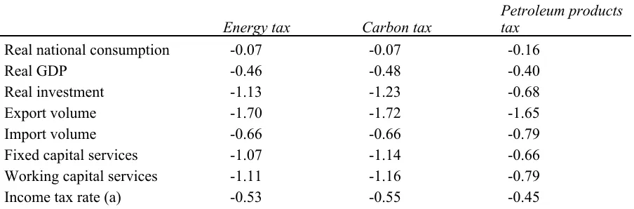
(17) reductions in carbon dioxide emission than in fossil fuel energy consumption. The carbon tax leads to greater reductions in both energy consumption and carbon dioxide emission than does the energy tax. But the difference is not great: the energy tax is about 70 per cent as effective as the carbon tax in reducing carbon dioxide emissions. The petroleum products tax however is much less effective Ñ about one thirtieth as effective as the carbon tax in reducing carbon dioxide emissions. Table 2: Estimated effects of energy, carbon and petroleum products taxes on fossil fuel energy use and carbon dioxide emissions (Percentage changes). Carbon dioxide emissions Fossil fuel energy use. Energy tax. Carbon tax. -13 -11. -17 -13. Petroleum products tax -0.6 -1.8. The energy and carbon taxes are quite similar in their macro effects, but the petroleum products tax differs considerably. Real national consumption falls by 0.07 per cent with the energy or carbon tax, but by 0.16 per cent with the petroleum products tax (table 3). The consumption falls reflect reductions in economic efficiency, measured in terms of market goods and services and disregarding any non-marketable environmental benefits. The higher costs associated with the petroleum products tax may reflect the high existing rates of petroleum excise; with petroleum products already highly taxed, further tax increases carry a steep efficiency penalty. Table 3: Estimated effects of energy, carbon and petroleum products taxes on selected macro variables (Percentage changes). Real national consumption Real GDP Real investment Export volume Import volume Fixed capital services Working capital services Income tax rate (a) (a). Energy tax -0.07 -0.46 -1.13 -1.70 -0.66 -1.07 -1.11 -0.53. Carbon tax -0.07 -0.48 -1.23 -1.72 -0.66 -1.14 -1.16 -0.55. Petroleum products tax -0.16 -0.40 -0.68 -1.65 -0.79 -0.66 -0.79 -0.45. Percentage point change. Against these costs should be set the non-market-measured benefits (if any) one attributes to the associated energy conservation and emission abatement (market measured benefits such as lower fuel bills are reflected in the income and consumption. 13.

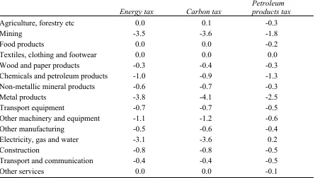
(18) results). Clearly from table 2 these benefits would be much greater with a carbon or energy tax than with a petroleum products tax. Unlike the costs shown above, which would be borne by Australians, any greenhouse abatement benefits would be enjoyed mainly outside Australia. The energy and carbon taxes would lead to falls in real GDP estimated at around 0.5 per cent. GDP falls largely because of a contraction in factor usage, specifically in usage of capital. This reflects structural change in the economy, away from more capital-intensive towards more labour-intensive industries. With constant labour employment, a reduction in the overall capital intensity of the economy implies a contraction in usage of capital. Fixed capital and working capital usage accordingly fall, each by around 1.1 per cent, with either the energy or the carbon tax. Capital usage also falls with the petroleum products tax, but less than with the energy and carbon taxes, by 0.7 per cent for fixed capital and 0.8 per cent for working capital. The fall in GDP with the petroleum products tax, at 0.4 per cent, is therefore less than with the energy or carbon taxes (0.5 per cent). The contraction in the capital stock reduces AustraliaÕs investment requirements; with little reduction in saving by Australians, this leads to a reduction in capital inflow from abroad. So foreign liabilities and income payments abroad both fall. The reduction in foreign income payments offsets the fall in factor income resulting from the contraction in the capital stock, with little net effect on household income. The falls in household income and consumption which are observed are driven mainly by efficiency losses. With the energy and carbon taxes the fall in real GDP is largely taken up on the expenditure side by falls in investment and exports (1.1, 1.7 per cent). Consumption also falls, but only by 0.1 per cent. The fall in investment reflects the contraction in the national capital stock. The fall in exports accomodates a reduction in income payments abroad, partly offset by a reduction in the surplus on capital account. With the carbon tax, there is less of a fall in investment (0.7 per cent), but a larger fall in consumption (0.2 per cent). The sectoral effects of the energy and carbon taxes are concentrated in the mining, metal products, and Ôelectricity, gas and waterÕ sectors. These show output contractions of around 3 to 4 per cent with both the energy and carbon taxes. Again the effects of the petroleum products tax are quite different: mining and metal products contract less, by 1.8 and 2.5 per cent, while electricity, gas and water actually expands slightly, by 0.2 per cent (table 4).. 14.

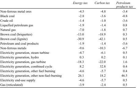
(19) Table 4: Estimated effects of energy, carbon and petroleum products taxes on activity, by broad sector (Percentage changes). Agriculture, forestry etc Mining Food products Textiles, clothing and footwear Wood and paper products Chemicals and petroleum products Non-metallic mineral products Metal products Transport equipment Other machinery and equipment Other manufacturing Electricity, gas and water Construction Transport and communication Other services. Energy tax 0.0 -3.5 0.0 0.0 -0.3 -1.0 -0.6 -3.8 -0.7 -1.1 -0.5 -3.1 -0.8 -0.4 0.0. Carbon tax 0.1 -3.6 0.0 0.0 -0.4 -0.9 -0.7 -4.1 -0.7 -1.2 -0.6 -3.6 -0.8 -0.4 0.0. Petroleum products tax -0.3 -1.8 -0.2 0.0 -0.3 -1.3 -0.3 -2.5 -0.5 -0.6 -0.4 0.2 -0.5 -0.5 -0.1. Looking at output changes at a more detailed level (table 5), the greatest reduction in output with the energy tax is in the brown coal industry (31 per cent). Brown coal is displaced by other less highly taxed fuels as an energy source for steam turbine power plant. Briquettes also suffer a severe output contraction (13 per cent) but other fossil fuels are much less affected. The loss of output in the metal products sector is concentrated in the energy-intensive and export-oriented non-ferrous metals industry. Electricity and reticulated gas output falls as the energy-intensive non-ferrous metals industry contracts and as end users adopt more fuel-economic methods. In the generation of base load power, the energy tax leads to switching away from steam turbine toward the more energy-efficient combined cycle technology. This switching leads to an expansion of 8 per cent in combined cycle generation. The initial level of combined cycle generation however is too low for the switching to have much effect on steam turbine generation. The 5 per cent fall in generation by this technology reflects mainly the overall decrease in base load power usage.. 15.

(20) Table 5: Estimated effects of energy, carbon and petroleum products taxes on activity in selected industries (Percentage changes). Non-ferrous metal ores Black coal Crude oil Liquefied petroleum gas Natural gas Brown coal (briquettes) Brown coal (lignite) Petroleum and coal products Non-ferrous metals Electricity generation, steam turbine Electricity generation, hydro Electricity generation, gas turbine Electricity generation, combined cycle Electricity generation, other fuel burning Electricity generation, other non-fuel-burning Electricity end-use supply Gas (reticulated). Energy tax. Carbon tax. -4.5 -2.8 -1.4 -1.9 -7.0 -13.0 -30.9 -1.9 -9.6 -4.7 0.3 -18.3 8.2 -4.6 26.1 -4.6 -3.9. -4.8 -3.6 -1.0 -1.4 -1.8 -18.9 -42.1 -1.4 -10.3 -6.1 0.2 -22.0 32.8 -5.7 18.2 -5.7 -2.4. Petroleum products tax -3.4 -0.8 -3.6 0.8 0.7 0.3 0.5 -5.6 -6.7 0.5 0.1 1.6 0.4 0.4 46.5 0.5 0.5. With the hydroelectricity generation level modelled as resource-determined, the reduction in peak load electricity generation falls entirely on gas turbine plant, which shows an output reduction of 18 per cent. In remote area electricity generation there is a strong increase in electricity generation from renewable energy sources (26 per cent), from a very low base. Output from Ôother fuel burningÕ plant falls 5 per cent, mainly because of the reduction in overall remote area power usage. The effects of the carbon tax on electricity generation are qualitatively similar to those of the energy tax, though it is more effective than the energy tax in promoting the substitution of combined cycle for steam turbine plant (with a 33 per cent increase in output from combined cycle plant), and less effective in promoting the substitution of Ôother non-fuel-burningÕ for Ôother fuel burningÕ plant. This is because the carbon tax falls more heavily than the energy tax on the coal used in steam turbine plant, but less heavily on the petroleum products used in Ôother fuel burningÕ. The carbon tax, being more heavily concentrated on the cheaper fuels than the energy tax, affects brown coal output more severely. Brown coal output falls by 42 per cent, as opposed to 30 per cent with the energy tax. Conversely natural gas usage falls only 2 per cent, as against 7 per cent with the energy tax. With the carbon tax, substitution. 16.

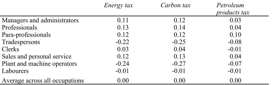
(21) of gas for coal in steam turbine plant is strong enough largely to offset the reduction in gas use in gas turbine plant. With the petroleum products tax a very different picture emerges. The only fossil fuel industries to suffer significant output reductions are the crude oil and petroleum products industries (3.6, 5.6 per cent). The non-ferrous metals industry, an intensive user not only of electricity but also of petroleum products, suffers an output decline of 7 per cent. Effects on electricity generation are generally small. End-use electricity consumption increases slightly (0.5 per cent) as electricity displaces petroleum products as a source of end-use energy. The electricity generation industry most greatly affected is Ôother non-fuel-burningÕ, which increases output by 44 per cent, being favoured by a rise in costs in the petroleum-products intensive Ôother fuel burningÕ electricity generation industry. The energy and carbon taxes lead to a slight skewing of labour employment away from blue-collar towards white-collar occupations (table 6). Employment of tradespersons and plant and machine operators falls (by around 0.2 to 0.3 per cent), while employment of managers and administrators, professionals and para-professionals rises slightly (by around 0.1 per cent). The employment effects of the petroleum products tax are generally smaller. The occupational employment results reflect changes in the industry structure of the economy; the industries that suffer from the energy and carbon taxes tend to have labour forces with a strong blue-collar component. Table 6: Estimated effects of energy, carbon and petroleum products taxes on employment, by occupation (Percentage changes) Energy tax Managers and administrators Professionals Para-professionals Tradespersons Clerks Sales and personal service Plant and machine operators Labourers Average across all occupations. Carbon tax. 0.11 0.13 0.12 -0.22 0.03 0.12 -0.24 -0.01 0.00. 0.12 0.14 0.12 -0.25 0.04 0.13 -0.27 -0.01 0.00. 17. Petroleum products tax 0.03 0.04 0.10 -0.08 -0.01 0.04 -0.07 -0.01 0.00.

(22) 4. Conclusions The main message from the exercise is that an energy tax could be a reasonably effective instrument for abating carbon dioxide emissions. While a carbon tax would be the theoretically ideal instrument for carbon dioxide abatement, any tax bearing heavily on the cheapest fossil fuels would be reasonably effective. An energy tax applying to all fossil fuels on an energy content basis would satisfy this requirement. Both in effectiveness in reducing greenhouse gas emissions and in non-greenhouse effects, there is not a great deal to choose between an energy tax and a carbon tax. For a given moderate level of tax revenue, an energy tax is not much less effective than an energy tax in reducing emissions. The reason is that the two taxes are quite similar in profile across fossil fuels; an energy tax is skewed against the cheaper fuels almost as heavily as a carbon tax. Looking at non-greenhouse effects, the costs of an energy tax and a carbon tax in terms of aggregate consumption are almost equal. The energy tax would involve somewhat less sectoral adjustment than a carbon tax, since it would bear less heavily on the brown coal industry; this is the other side of the coin to the somewhat lower effectiveness of the energy tax in reducing greenhouse gas emissions. By contrast a tax on petroleum products is both much less greenhouse effective and considerably more costly than either an energy or a carbon tax. At the level of tax revenue considered here it is about one sixth as effective as an energy tax in reducing greenhouse gas emissions, and one eighth as effective as a carbon tax. But the cost in terms of market goods and services is more than twice as high as with an energy or a carbon tax. The petroleum tax is levied on relatively expensive fuels, has relatively little impact on their price, and does little to encourage greater energy efficiency. Furthermore it does not encourage the substitution of low-emission for high emission fuels, which is one of the main sources of emission abatement with the energy and carbon taxes. It is similarly ineffective in promoting fuel conservation. The petroleum tax however does not have nearly such severe sectoral effects as the carbon and energy taxes. The emission abatement with the carbon and energy taxes involves strong substitution away from brown coal, and a severe contraction in brown coal mining. The petroleum tax has no such severe sectoral effects. The simulation results have several implications for policy discussion. They suggest that a comprehensive energy tax can reasonably be represented as ÔgreenhousefriendlyÕ, but a petroleum products tax cannot (this is consistent with the 1993-94 Australian budget papers, which proposed petroleum excise increases on nongreenhouse grounds). Similarly, if fuel conservation is taken to apply to all fossil fuels. 18.

(23) equally, then fuel conservation and greenhouse gas abatement would be almost equivalent goals, inasmuch as efficient measures to achieve either goal would typically serve both. But if fuel conservation is taken to entail primarily the conservation of oil and gas (a natural interpretation in Australia, with its large coal reserves) this equivalence disappears; efficient fuel conserving measures would have little effect on carbon dioxide emissions, and vice versa. Finally the results reinforce a point made by previous studies (e.g. IC 1991, Jones, Naughten et al. 1991) that strong greenhouse abatement action in Australia would be liable involve large reductions in usage of coal, especially brown coal. Dollar for dollar, savings in usage of more expensive fuels such as petroleum would have relatively little anti-greenhouse effect. The simulation results must as usual be qualified by a recognition of the great uncertainty in key behavioural parameters and the potential for further refinement in the structure of the model. Another qualification necessary in the present instance is that some of the main conclusions may be specific to the level of tax revenue on which the comparisons are based. For example, it may be that at a higher level of tax revenue, the relative costliness of the petroleum tax compared to the energy and carbon taxes may be reversed. On the other hand, for the level of tax revenue chosen, the general tendency of the conclusions largely reflects known price relationships between different fuels, and seems likely to be robust with respect to a wide range of model variations.. References Adams, P.D. and Dixon, P.B. 1992, Disaggregating Oil, Gas and Brown Coal, Monash University Centre of Policy Studies, mimeo. Australian Bureau of Statistics 1990a, Australian National Accounts, Input-Output Tables, 1986-87, Cat. No. 5209.0. Australian Bureau of Statistics 1990b, Australian National Accounts, Input-Output Tables, Commodity Details, 1986-87, Cat. No. 5215.0. Commonwealth of Australia 1992, National Greenhouse Response Strategy, AGPS, Canberra. Dawkins, J. and Willis, R. 1993, Budget Statements 1993-94, AGPS, Canberra. Dee, P.S. 1989, FH-ORANI: A Fiscal ORANI with Horridge Extension, University of Melbourne IMPACT Project Preliminary Working Paper No. OP-66. Dixon, P.B., Parmenter, B.R., Sutton, J., and Vincent, D.P. 1982, ORANI: A Multisectoral Model of the Australian Economy, North-Holland, Amsterdam.. 19.

(24) Electricity Supply Association of Australia Ltd 1993, Electricity Australia 1993, Electricity Supply Association of Australia Ltd, Sydney, Melbourne, and Canberra. Harrison, J. and Pearson, K. 1993a, An Introduction to GEMPACK, Monash University IMPACT Project GEMPACK Document No. GPD-1. Harrison, J. and Pearson, K. 1993b, UserÕs Guide to TABLO and TABLO-Generated Programs, Monash University IMPACT Project GEMPACK Document No. GPD-2. Horridge, M. 1985, Long-Run Closure of ORANI: First Implementation, University of Melbourne IMPACT Project Preliminary Working Paper No. OP-50. Horridge, J.M., Parmenter B.R. and Pearson K.R. 1993, ÔORANI-F: A General Equilibrium Model of the Australian EconomyÕ, Economic and Financial Computing Vol. 3 No. 2. Intelligent Energy Systems Pty Ltd 1991, Comparative Costs of Producing Energy from Renewable and Non-renewable Sources in Australia, report prepared for the Energy Production Working Group under the Ecologically Sustainable Development Programme. Industry Commission 1991, Costs and Benefits of Reducing Greenhouse Gas Emissions, Report No. 15, AGPS, Canberra. Jones, B., Bush, S., Kanakaratnam, A., Leonard, M., and Gillan, P. 1991, Projections of Energy Demand and Supply, Australia 1990-91 to 2004-05, AGPS, Canberra. Jones, B., Naughten, B., Peng, Z.-Y., and Watts, S. 1991, Costs of Reducing Carbon Dioxide Emissions from the Australian Energy Sector, Report to the Ecologically Sustainable Development Working Groups. McDougall, R.A. 1993a, Incorporating International Capital Mobility into SALTER , Industry Commission SALTER Working Paper No. 21. ÑÑÑÑ 1993b, Flexibly Nested Production Functions: Implementation for MONASH, Monash University COPS/IMPACT Preliminary Working Paper No. IP-57. Nicoletti, G. and Oliveira-Martins, J. 1992, Global Effects of the European Carbon Tax, Organisation for Economic Co-Operation and Development, Economics Department Working Paper No. 125. Pearce, D. 1991, ÔThe Role of Carbon Taxes in Adjusting to Global WarmingÕ, Economic Journal, Vol. 101, pp. 938-48. Powell, A.A. and Snape R.H. 1993, ÔThe Contribution of Applied General Equilibrium Analysis to Policy Reform in AustraliaÕ, Journal of Policy Modeling Vol. 15 No. 4. Wallace, C. 1993, ÔCars may rally to the rescueÕ, Australian Financial Review, 5 July.. 20.

(25) Appendix 1: Changes to the theoretical structure Sets SET COM # Commodities # MAXIMUM size 125 READ elements from file PARAMS header "SC00"; SET MARGCOM # Margin Commodities # MAXIMUM size 9 READ elements from file PARAMS header "SCM0"; ! These margin commodities are : 95 - Wholesale trade 96 - Retail trade 99 - Road transport 100 - Rail and other transport 101 - Water transport 102 - Air transport 103 - Services to transport 108 - Insurance and services 117 - Restaurants, hotels ! SUBSET MARGCOM is subset of COM; SET TRANS_MARG # Transport margin commodities # MAXIMUM size 4 READ elements from file PARAMS header "SCMT"; ! These transport margin commodities are : 105 - Road transport 106 - Rail and other transport 107 - Water transport 108 - Air transport ! SUBSET TRANS_MARG is subset of COM; SUBSET TRANS_MARG is subset of MARGCOM; SET NONMARGCOM # Non-Margin Commodities # MAXIMUM size 116 READ elements from file PARAMS header "SCN0"; SUBSET NONMARGCOM is subset of COM; SET IND # Industries # MAXIMUM size 123 READ elements from file PARAMS header "SI00"; SET FAC. # Primary factors # (labour,capital,land);. SET SOURCE # Domestic/Imported # ( domestic,imported ); SET BAD # carbon dioxide, energy in fossil fuels, energy in petroleum products # (CO2, fossil_fuel, petr_prods);. Variables used in new equations VARIABLE !. Scalar variables ----------------. !. ah # household net wealth (CHANGE) apc # household average propensity to consume ! percentage point change !. 21. #; #;.

(26) c # household consumption expenditure #; gdpexp # expenditure on gross domestic product #; labrev # labour earnings #; lndrev # land earnings #; othnom # government consumption expenditure etc. #; phi # exchange Rate #; (CHANGE) qdh # household debt ratio #; ! ratio of household debt to purchase value of productive assets ! ! percentage point change ! (CHANGE) qih # household interest ratio #; ! ratio of household interest payments to factor income ! ! percentage point change ! (CHANGE) r0dha # rate of interest on household debt, after tax #; ! percentage point change ! (CHANGE) r0dhb # rate of interest on household debt, before tax #; ! percentage point change ! (CHANGE) rsg # government current surplus ratio #; ! ratio of government current surplus to GDP ! ! percentage point change ! ! (govt current surplus) = tax - (govt consumption expenditure) ! (CHANGE) rty # income tax rate #; ! percentage point change ! t_ # tax #; taxrate1 # shift in power of commodity tax on intermediate usage #; taxrate2 # shift in power of commodity tax on investment usage #; taxrate3 # shift in power of commodity tax on household consumption #; taxrate5 # shift in power of commodity tax on government consumption #; (CHANGE) taxrevbads # carbon tax revenue ($ million) #; tc # commodity tax #; tn # non-commodity indirect tax #; ty # income tax #; vs # value of physical assets #; vskf # value of fixed capital #; vskw # value of working capital #; vsn # value of land #; xi3 # consumer price index #; xiah # price index for household assets #; xikf # price index for fixed capital #; xikw # price index for working capital #; xin # price index for land #; xiworld # proxy for World Price Index #; yh # household income #; yhd # household disposable income #; yhf # household factor income #; ykf # fixed capital income #; ykw # working capital income #; !. Vector variables ----------------. !. 22.

(27) (ALL,j,IND) fpiwi(j) # (CHANGE) (ALL,j,IND) fr0a(j) # ! percentage point change (ALL,j,IND) fy(j) # (ALL,i,COM) p0dom(i) # (ALL,j,IND) p1kwi(j) # (ALL,i,COM) p74(i) # (ALL,j,IND) pifi(j) # (ALL,j,IND) pini(j) # (ALL,j,IND) piwi(j) # (ALL,i,COM) powtax(i) # (CHANGE) (ALL,j,IND) r0a(j) # ! Percentage point change (CHANGE) (ALL,j,IND) r0b(j) # ! Percentage point change (CHANGE) (ALL,b,BAD) ratetaxbads(b) # (ALL,j,IND) x1kwi(j) # (ALL,i,COM) x4(i) # (ALL,j,IND) y(j) # (ALL,j,IND) ykfi(j) # !. Matrix variables ----------------. shift in rental working capital rental. #;. shift in equity premium ! investment shift basic price of domestic product rental price of working capital price of transporting i for export purchase price of fixed capital purchase price of land purchase price of working capital shift in power of commodity tax. #;. rate of return after tax !. #;. rate of return before tax !. #;. bads tax rate, specific usage of working capital, by industry export volume gross investment, by industry fixed capital income, by industry. #; #; #; #; #;. #; #; #; #; #; #; #; #;. !. (ALL,i,COM)(ALL,s,SOURCE)(ALL,j,IND)(ALL,r,MARGCOM) a1marg(i,s,j,r) # margins tech.change - intermediate usage #; (ALL,i,COM)(ALL,s,SOURCE)(ALL,j,IND)(ALL,r,MARGCOM) a2marg(i,s,j,r) # margins tech.change - investment usage #; (ALL,i,COM) (ALL,s,SOURCE) (ALL,r,MARGCOM) a3marg(i,s,r) # margins tech.change - household consumption #; (ALL,i,COM) (ALL,r,MARGCOM) a4marg(i,r) # margins tech.change - exports #; (ALL,i,COM)(ALL,s,SOURCE)(ALL,r,MARGCOM) a5marg(i,s,r) # margins tech.change - government consumption etc #; (ALL,i,COM)(ALL,s,SOURCE) p0(i,s) # basic price #; (ALL,j,IND)(ALL,v,FAC) p1fi(j,v) # price / price index for factor v employed in industry j #; (ALL, i, COM) (ALL, s, SOURCE) (ALL, j, IND) p71(i,s,j) # price of transporting i from s for intermediate usage by j #; (ALL, i, COM) (ALL, s, SOURCE) (ALL, j, IND) p72(i,s,j) # price of transporting i from s for capital formation by j #; (ALL, i, COM) (ALL, s, SOURCE) p73(i,s) # price of transporting i from s for household consumption #; (ALL, i, COM) (ALL, s, SOURCE) p75(i,s) # price of transporting i from s for "other" use #; (ALL,i,COM)(ALL,s,SOURCE)(ALL,j,IND) powtax1(i,s,j) # shift in power of commodity tax on intermediate usage #; (ALL,i,COM)(ALL,s,SOURCE)(ALL,j,IND) powtax2(i,s,j) # shift in power of commodity tax on investment usage #; (ALL,i,COM)(ALL,s,SOURCE) powtax3(i,s) # shift in power of commodity tax on household consumption #; (ALL,i,COM)(ALL,s,SOURCE). 23.

(28) powtax5(i,s) # shift in power of commodity tax on government consumption #; (CHANGE) (ALL,s,SOURCE) (ALL, b, BAD) (ALL,i,COM) radvalbads(i,b,s) # emission tax rate, ad valorem, percentage point #; (ALL,j,IND)(ALL,v,FAC) x1fi(j,v) # employment of factor v in industry j #; (ALL,i,COM)(ALL,s,SOURCE)(ALL,j,IND) x1isc(i,s,j) # intermediate usage #; (ALL,i,COM)(ALL,s,SOURCE)(ALL,j,IND)(ALL,r,MARGCOM) x1marg(i,s,j,r) # Margin usage on flow to intermediate usage #; (ALL,i,COM)(ALL,s,SOURCE)(ALL,j,IND) x2isc(i,s,j) # investment usage #; (ALL,i,COM)(ALL,s,SOURCE)(ALL,j,IND)(ALL,r,MARGCOM) x2marg(i,s,j,r) # margin usage on flow to investment usage #; (ALL,i,COM)(ALL,s,SOURCE) x3sc(i,s) # household consumption #; (ALL,i,COM)(ALL,s,SOURCE)(ALL,r,MARGCOM) x3marg(i,s,r) # margin usage on flow to household consumption #; (ALL,i,COM)(ALL,r,MARGCOM) x4marg(i,r) # margin usage on export flow #; (ALL,i,COM)(ALL,s,SOURCE) x5sc(i,s) # government consumption etc. #; (ALL,i,COM)(ALL,s,SOURCE)(ALL,r,MARGCOM) x5marg(i,s,r) # margin usage on government consumption etc. flow #;. Coefficients used in new equations !. Coefficients read from existing data ------------------------------------. !. COEFFICIENT (ALL,i,COM)(ALL,s,SOURCE)(ALL,j,IND) BAS1(i,s,j) # intermediate usage at basic values #; COEFFICIENT (ALL,i,COM)(ALL,s,SOURCE)(ALL,j,IND) BAS2(i,s,j) # usage in capital formation at basic values #; COEFFICIENT (ALL,i,COM)(ALL,s,SOURCE) BAS3(i,s) # household consumption at basic values #; COEFFICIENT (ALL,i,COM)(ALL,s,SOURCE) BAS5(i,s) # government consumption etc. at basic values #; COEFFICIENT (ALL,i,COM)(ALL,s,SOURCE)(ALL,j,IND)(ALL,r,MARGCOM) MAR1(i,s,j,r) # margin on intermediate usage #; COEFFICIENT (ALL,i,COM)(ALL,s,SOURCE)(ALL,j,IND)(ALL,r,MARGCOM) MAR2(i,s,j,r) # margin on investment usage #; COEFFICIENT (ALL,i,COM)(ALL,s,SOURCE)(ALL,r,MARGCOM) MAR3(i,s,r) # margin on household consumption #; COEFFICIENT (ALL,i,COM)(ALL,r,MARGCOM) MAR4(i,r) # margin on exports #; COEFFICIENT (ALL,i,COM)(ALL,s,SOURCE)(ALL,r,MARGCOM) MAR5(i,s,r) # margin on government consumption etc #; COEFFICIENT (ALL,i,COM)(ALL,s,SOURCE)(ALL,j,IND) TAX1(i,s,j) # commodity tax on intermediate usage #; COEFFICIENT (ALL,i,COM)(ALL,s,SOURCE)(ALL,j,IND) TAX2(i,s,j) # commodity tax on investment usage #;. 24.

(29) COEFFICIENT (ALL,i,COM)(ALL,s,SOURCE) TAX3(i,s) # commodity tax on household consumption #; COEFFICIENT (ALL,i,COM)(ALL,s,SOURCE) TAX5(i,s) # commodity tax on government consumption etc #; !. Coefficients read from data newly added to the model ----------------------------------------------------. !. COEFFICIENT TAXY # Income tax #; READ TAXY from file FID header "FS02"; COEFFICIENT (ALL, j, IND) V1KWi(j) # Earnings of working capital #; READ V1KWi from file FID header "FS04"; COEFFICIENT (ALL, j, IND) TAXNi(j) # Non-commodity indirect tax, by industry #; READ TAXNi from file FID header "FS05"; COEFFICIENT PAYHI # Net interest payments by households #; READ PAYHI from file FID header "FS06"; COEFFICIENT RORDHA # Interest rate on household debt, net of tax #; READ RORDHA from file FID header "FS07"; COEFFICIENT RATGH # Rate of growth in household disposable income #; READ RATGH from file FID header "FS08"; COEFFICIENT (ALL,s,SOURCE) (ALL, b, BAD) (ALL,i,COM) EMISS_INTENS(i,b,s) # emission intensity by bad, commodity, and source (physical unit/ $m) #; READ EMISS_INTENS FROM FILE fid HEADER "FS09"; COEFFICIENT (ALL, b, BAD) RTTXBb(b) # carbon tax rate ($ million / physical unit) #; READ RTTXBb FROM FILE fid HEADER "FS10"; COEFFICIENT TAU # Length of run #; READ TAU from file PARAMS header "PS01"; !. Emission release rate for commodity i in use k is defined as (emission of ÔbadsÕ from commodity i in use k) /(bads content of commodity i) !. COEFFICIENT (ALL,i,COM)(ALL,j,IND) SHRF1(i,j) # emission release rate in intermediate usage #; READ SHRF1 FROM FILE PARAMS HEADER "PEE1"; COEFFICIENT (ALL,i,COM)(ALL,j,IND) SHRF2(i,j) # emission release rate in capital formation #; READ SHRF2 FROM FILE PARAMS HEADER "PEE2"; COEFFICIENT (ALL,i,COM) SHRF3(i) # emission release rate in household consumption #; READ SHRF3 FROM FILE PARAMS HEADER "PEE3"; COEFFICIENT (ALL,i,COM) SHRF5(i) # emission release rate in government consumption #; READ SHRF5 FROM FILE PARAMS HEADER "PEE4";. 25.

(30) !. Calculated coefficients from standard model -------------------------------------------. COEFFICIENT AGGCON. !. # household consumption expenditure #;. COEFFICIENT AGGOTH # government consumption expenditure etc. #; COEFFICIENT GDPEX # expenditure on gross domestic product #; COEFFICIENT (ALL,v,FAC)(ALL,j,IND) V1fi(j,v) # earnings of factor v in industry j #; COEFFICIENT FORMULA. AGGLAB # labour earnings #; AGGLAB = SUM(j, IND, V1fi(j,"labour"));. COEFFICIENT FORMULA. AGGLND # land earnings #; AGGLND = SUM(j, IND, V1fi(j,"land"));. COEFFICIENT TAXC # commodity tax #; COEFFICIENT TINY # Arbitrary small number #; FORMULA TINY = 0.000000000001; !. Calculated coefficients newly added to the model ------------------------------------------------. !. COEFFICIENT (ALL, j, IND) INCKFi(j) # Earnings of fixed capital #; FORMULA (ALL, j, IND) INCKFi(j) = V1fi(j,"capital") - DEPR(j); COEFFICIENT INCKF # Income from fixed capital #; FORMULA INCKF = SUM(j, IND, INCKFi(j)); COEFFICIENT V1KW # Working capital income #; FORMULA V1KW = SUM(j, IND, V1KWi(j)); COEFFICIENT INCHF # Household factor income #; FORMULA INCHF = AGGLAB + INCKF + AGGLND + V1KW; COEFFICIENT INCH # Household income #; FORMULA INCH = INCHF - PAYHI; COEFFICIENT INCHD # Household disposable income #; FORMULA INCHD = INCH - TAXY; COEFFICIENT ROTY # income tax rate #; FORMULA ROTY = TAXY/INCH; COEFFICIENT RORDHB # Interest rate on household debt #; FORMULA RORDHB = RORDHA/(1 - ROTY); COEFFICIENT (ALL, j, IND) VALSKFi(j) # Value of capital stock #; FORMULA (ALL, j, IND) VALSKFi(j) = (1 - ROTY)*(V1fi(j,"capital") - DEPR(j)) / RORA(j);. 26.

(31) COEFFICIENT VALSKF # Purchase value of fixed capital #; FORMULA VALSKF = SUM(j, IND, VALSKFi(j)); COEFFICIENT (ALL, j, IND) VALSKWi(j) # Purchase value of working capital, by industry #; FORMULA (ALL, j, IND) VALSKWi(j) = (1 - ROTY)*V1KWi(j)/RORA(j); COEFFICIENT VALSKW # Purchase value of working capital #; FORMULA VALSKW = SUM(j, IND, VALSKWi(j)); COEFFICIENT (ALL, j, IND) VALSNi(j) # Purchase value of land, by industry #; FORMULA (ALL, j, IND) VALSNi(j) = (1 - ROTY)*V1fi(j,"land")/RORA(j); COEFFICIENT VALSN # Purchase value of land #; FORMULA VALSN = SUM(j, IND, VALSNi(j)); COEFFICIENT ASSP # Physical assets #; FORMULA ASSP = VALSKF + VALSKW + VALSN; COEFFICIENT VALSDH # Household debt #; FORMULA VALSDH = (1 - ROTY)*PAYHI/RORDHA; COEFFICIENT ASSH # Household assets #; FORMULA ASSH = ASSP - VALSDH; COEFFICIENT TAXC # aggregate commodity tax revenue #; FORMULA TAXC = AGGTAX1 + AGGTAX2 + AGGTAX3 + AGGTAX4 + AGGTAX5 + AGGTAXM; COEFFICIENT TAXN # Non-commodity indirect tax #; FORMULA TAXN = SUM(j, IND, TAXNi(j)); COEFFICIENT (ALL,r,MARGCOM) TRANS_DUMM(r) # Dummy coefficient identifying transport margins #; FORMULA (ALL,r,MARGCOM) TRANS_DUMM(r) = 0.0; FORMULA (ALL,r,TRANS_MARG) TRANS_DUMM(r) = 1.0;. Equations added for long-run comparative statics !. Consumption behaviour ---------------------. !. EQUATION HHOLD_CONSN_SPENDING # Household consumption expenditure # AGGCON*c = INCHD*apc + AGGCON*yhd; !. Investment ----------. !. EQUATION TERM_INV # terminal point investment # (ALL, j, IND) y(j) = x1fi(j,"capital") + fy(j);. 27.

(32) !. Rate of return relations ------------------------. !. COEFFICIENT (ALL, j, IND) RORG(j) # Gross rate of return #; ZERODIVIDE DEFAULT 0.2; FORMULA (ALL, j, IND) RORG(j) = V1fi(j,"capital") / VALSKFi(j); COEFFICIENT (ALL, j, IND) RORB(j) # Rate of return before tax #; FORMULA (ALL, j, IND) RORB(j) = [V1fi(j,"capital") - DEPR(j)]/VALSKFi(j); EQUATION ROR_BEFORE_TAX # E.P.9: Rate of return before tax # (ALL, j, IND) r0b(j) = RORG(j)*(p1fi(j,"capital") - pifi(j)); EQUATION ROR_AFTER_TAX # E.P.10: Rate of return after tax # (ALL, j, IND) r0a(j) = -RORB(j)*rty + (1 - ROTY)*r0b(j); EQUATION PURCHASE_P_WORKING_K # E.P.11: Purchase price of working capital # (ALL, j, IND) piwi(j) = xi3 + fpiwi(j); EQUATION RENTAL_P_WORKING_K # E.P.12: Rental price of working capital # (ALL, j, IND) r0b(j) = RORB(j)*(p1kwi(j) - piwi(j)); EQUATION PURCHASE_PRICE_LAND # E.P.13: Purchase price of land # (ALL, j, IND) r0b(j) = RORB(j)*(p1fi(j,"land") - pini(j)); EQUATION ROI_HOUS_NET # after-tax rate of interest on household debt # r0dha = -RORDHB*rty + (1 - ROTY)*r0dhb; !. Household wealth accumulation -----------------------------. !. EQUATION FIXED_K_P_INDEX # Price index for fixed capital # VALSKF*xikf = SUM(j, IND, VALSKFi(j)*pifi(j)); EQUATION WORKING_K_P_INDEX # Price index for working capital # VALSKW*xikw = SUM(j, IND, VALSKWi(j)*piwi(j)); EQUATION LAND_PRICE_INDEX VALSN*xin = SUM(j, IND, VALSNi(j)*pini(j)); EQUATION HHOLD_ASSET_P_INDEX # Household asset price index # ASSH*xiah = VALSKF*xikf + VALSKW*xikw + VALSN*xin - VALSDH*(xiworld + phi); COEFFICIENT SAVH # Household saving #; FORMULA SAVH = INCHD - AGGCON; COEFFICIENT FACGH # Household income growth factor #; FORMULA FACGH = RATGH*TAU; COEFFICIENT MSCAWH1 # Household wealth accumulation coefficient #;. 28.

(33) ZERODIVIDE DEFAULT 1.0; FORMULA MSCAWH1 = (1.0 - exp(-FACGH))/FACGH; COEFFICIENT MSCAWH2 # Household wealth accumulation coefficient #; ZERODIVIDE DEFAULT 0.5; FORMULA MSCAWH2 = (FACGH - 1.0 + exp(-FACGH))/(FACGH^2); EQUATION HHOLD_WEALTH_ACCN # Household wealth accumulation # ASSH*ah = (ASSH - MSCAWH1*SAVH*TAU)*xiah - MSCAWH1*INCHD*TAU*apc + MSCAWH1*SAVH*TAU*xi3 + MSCAWH2*SAVH*TAU*(yhd - xi3); !. Household income ----------------. !. COEFFICIENT (ALL, j, IND) MSCQi(j) # Ratio of gross to net returns to fixed capital #; ZERODIVIDE DEFAULT 1.7; FORMULA (ALL, j, IND) MSCQi(j) = V1fi(j,"capital")/INCKFi(j); EQUATION FIXED_K_Y_IND # Income from fixed capital, by industry # (ALL, j, IND) ykfi(j) = MSCQi(j)*p1fi(j,"capital") - (MSCQi(j) - 1.0)*pifi(j) + x1fi(j,"capital"); EQUATION FIXED_CAPITAL_Y # Income from fixed capital # INCKF*ykf = SUM(j, IND, INCKFi(j)*ykfi(j)); EQUATION WORKING_CAPITAL_Y # Working capital income # V1KW * ykw = SUM(j, IND, V1KWi(j )* (p1kwi(j) + x1kwi(j))); EQUATION HHOLD_FACTOR_INCOME INCHF * yhf = AGGLAB * labrev + INCKF*ykf + AGGLND * lndrev + V1KW * ykw; EQUATION PAY_INT_HHOLD # Interest payments by households # INCHF*qih + PAYHI*yhf = VALSDH*r0dhb + RORDHB*ASSP*qdh + PAYHI*vs; EQUATION HOUSEHOLD_INCOME INCH*yh = INCH*yhf - INCHF*qih; EQUATION HHOLD_DISPOSABLE_Y # Household disposable income # INCHD * yhd = -INCH * rty + INCHD * yh; !. Household balance sheet -----------------------. !. EQUATION PURCHASE_V_FIXED_K # Value of stock of fixed capital # VALSKF*vskf = SUM(j, IND, VALSKFi(j)*(pifi(j) + x1fi(j,"capital"))); EQUATION PURCHASE_V_WORKING_K # Value of stock of working capital # VALSKW*vskw = SUM(j, IND, VALSKWi(j)*(piwi(j) + x1kwi(j)));. 29.

(34) EQUATION PURCHASE_V_LAND # Value of stock of land # VALSN*vsn = SUM(j, IND, VALSNi(j)*(pini(j) + x1fi(j,"land"))); EQUATION PHYSICAL_ASSETS # Value of domestic physical assets # ASSP*vs = VALSKF*vskf + VALSKW*vskw + VALSN*vsn; EQUATION HHOLD_WEALTH_IDENT # Household wealth identity # ASSH*ah = ASSH*vs - ASSP*qdh; !. Government surplus/deficit --------------------------. EQUATION INCOME_TAX. !. TAXY * ty = INCH * rty + TAXY * yh;. COEFFICIENT TAX # Tax #; FORMULA TAX = TAXY + TAXC + TAXN; EQUATION TOTAL_TAX. TAX * t_ = TAXY * ty + TAXC * tc + TAXN * tn;. COEFFICIENT SGOV # Government surplus #; ! Surplus of tax revenue over government consumption expenditure ! FORMULA SGOV = TAX - AGGOTH; EQUATION GOVT_SURPLUS GDPEX * rsg + SGOV * gdpexp = TAX * t_ - AGGOTH * othnom; !. Equilibium condition for rates of return ----------------------------------------. !. EQUATION EQUIL_ROR # equilibrium condition for rates of return # (all, j, IND) r0a(j) = r0dha + fr0a(j);. New energy-related equations ! Emission taxation -----------------. !. COEFFICIENT (ALL, b, BAD) Q_EMISS(b) # bads emissions #; FORMULA (ALL, b, BAD) Q_EMISS(b) = SUM(i,COM, SUM(s,SOURCE, EMISS_INTENS(i,b,s) * [ SUM(j, IND, SHRF1(i,j) * BAS1(i,s,j)) + SUM(j, IND, SHRF2(i,j) * BAS2(i,s,j)) + SHRF3(i)*BAS3(i,s) + SHRF5(i) * BAS5(i,s)])) + TINY; EQUATION EMISSIONS # carbon dioxide emissions # (ALL, b, BAD) Q_EMISS(b)*b_(b). 30.

(35) = SUM(i, COM, SUM(s, SOURCE, EMISS_INTENS(i,b,s) * [ SUM(j, IND, SHRF1(i,j) + SUM(j, IND, SHRF2(i,j) + SHRF3(i) * BAS3(i,s) * + SHRF5(i) * BAS5(i,s) *. * BAS1(i,s,j) * x1isc(i,s,j)) * BAS2(i,s,j) * x2isc(i,s,j)) x3sc(i,s) x5sc(i,s)]));. COEFFICIENT (ALL, b, BAD) RVTXBb(b) # emissions tax revenue, $m #; FORMULA (ALL, B, BAD) RVTXBb(b) = RTTXBb(b)*Q_EMISS(b); EQUATION BADS_TAX_REV # bads tax revenue # taxrevbads = SUM(b, BAD, Q_EMISS(b)*ratetaxbads(b)) + (1/100.0)*SUM(b, BAD, RVTXBb(b)*b_(b)); EQUATION RATE_ADVAL_CARBTAX # E.TA.1: Ad valorem equivalent rate of carbon tax # (ALL,i,COM)(ALL, b, BAD)(ALL,s,SOURCE) radvalbads(i,b,s) = EMISS_INTENS(i,b,s)*(100*ratetaxbads(b) - RTTXBb(b)*p0(i,s)); !. Factor of 100 yields radvalbads as a percentage point change.. !. EQUATION POW_INT_TAX # E.TA.2: Power of tax on sales to intermediate # (ALL,i,COM)(ALL,s,SOURCE)(ALL,j,IND) [BAS1(i,s,j) + TAX1(i,s,j) + TINY] * [powtax1(i,s,j) - powtax(i) - taxrate1] = SHRF1(i,j) * BAS1(i,s,j) * SUM(b, BAD, radvalbads(i,b,s)); EQUATION POW_CAP_TAX # E.TA.3: Power of tax on sales to investment # (ALL,i,COM)(ALL,s,SOURCE)(ALL,j,IND) [BAS2(i,s,j) + TAX2(i,s,j) + TINY] * [powtax2(i,s,j) - powtax(i) - taxrate2] = SHRF2(i,j) * BAS2(i,s,j) * SUM(b, BAD, radvalbads(i,b,s)); EQUATION POW_HOUS_TAX # E.TA.4: Power of tax on sales to households # (ALL,i,COM)(ALL,s,SOURCE) (BAS3(i,s) + TAX3(i,s) + TINY)*(powtax3(i,s) - powtax(i) - taxrate3) = SHRF3(i)*BAS3(i,s)*SUM(b, BAD, radvalbads(i,b,s)); ! powtax4(i) is normally endogenous for some commodities ! EQUATION POW_OTH_TAX # E.TA.5: Power of tax on sales to other # (ALL,i,COM)(ALL,s,SOURCE) (BAS5(i,s) + TAX5(i,s) + TINY)*(powtax5(i,s) - powtax(i) - taxrate5) = SHRF5(i)*BAS5(i,s)*SUM(b, BAD, radvalbads(i,b,s)); ! Intermodal substitution in margin use of transport services ----------------------------------------------------------EQUATION PTRANS_INT # E.TR.1 Price of transport margin in intermediate usage # (ALL,i,COM)(ALL,j,IND)(ALL,s,SOURCE) (TRANS_MARG1(i,s,j) + TINY)*p71(i,s,j). 31. !.

(36) = SUM(r, TRANS_MARG, MAR1(i,s,j,r)*(p0dom(r) + a1marg(i,s,j,r))); EQUATION MARG_INT # E.TR.2 Margins on intermediate usage # (ALL,i,COM)(ALL,j,ind)(ALL,s,SOURCE)(ALL,r,MARGCOM) x1marg(i,s,j,r) - a1marg(i,s,j,r) = x1isc(i,s,j) - TRANS_DUMM(r)*SIGMA7(i)*(p0dom(r) + a1marg(i,s,j,r) - p71(i,s,j)); EQUATION PTRANS_INV # E.TR.3 Price of transport margin for capital formation # (ALL,i,COM)(ALL,j,IND)(ALL,s,SOURCE) (TRANS_MARG2(i,s,j) + TINY)*p72(i,s,j) = SUM(r,TRANS_MARG,MAR2(i,s,j,r)*(p0dom(r) + a2marg(i,s,j,r))); EQUATION MARG_INV # E.TR.4 Margins for capital formation # (ALL,i,COM)(ALL,j,ind)(ALL,s,SOURCE)(ALL,r,MARGCOM) x2marg(i,s,j,r) - a2marg(i,s,j,r) = x2isc(i,s,j) - TRANS_DUMM(r)*SIGMA7(i)*(p0dom(r) + a2marg(i,s,j,r) - p72(i,s,j)); EQUATION PTRANS_HHLD # E.TR.5 Price of transport margin for household consumption # (ALL,i,COM)(ALL,s,SOURCE) (TRANS_MARG3(i,s) + TINY)*p73(i,s) = SUM(r,TRANS_MARG,MAR3(i,s,r)*(p0dom(r) + a3marg(i,s,r))); EQUATION MARG_HHLD # E.TR.6 Transport margins for household consumption # (ALL,i,COM)(ALL,s,SOURCE)(ALL,r,MARGCOM) x3marg(i,s,r) - a3marg(i,s,r) = x3sc(i,s) - TRANS_DUMM(r)*SIGMA7(i)*(p0dom(r) + a3marg(i,s,r) - p73(i,s)); EQUATION PTRANS_EXP # E.TR.7 Price of transport margin for exports # (ALL,i,COM) (TRANS_MARG4(i)+ TINY)*p74(i) = SUM(r,TRANS_MARG,MAR4(i,r)*(p0dom(r) + a4marg(i,r))); EQUATION MARG_EXP # E.TR.8 Transport margins for exports # (ALL,i,COM)(ALL,r,MARGCOM) x4marg(i,r) - a4marg(i,r) = x4(i) - TRANS_DUMM(r)*SIGMA7(i)*(p0dom(r) + a4marg(i,r) - p74(i)); EQUATION PTRANS_OTH # E.TR.9 Price of transport margin for "other" use # (ALL,i,COM)(ALL,s,SOURCE) (TRANS_MARG5(i,s) + TINY)*p75(i,s) = SUM(r,TRANS_MARG,MAR5(i,s,r)*(p0dom(r) + a5marg(i,s,r))); EQUATION MARG_OTH # E.TR.10 Transport margins for "other" use # (ALL,i,COM)(ALL,s,SOURCE)(ALL,r,MARGCOM) x5marg(i,s,r) - a5marg(i,s,r) = x5sc(i,s) - TRANS_DUMM(r)*SIGMA7(i)*(p0dom(r) + a5marg(i,s,r) - p75(i,s));. 32.

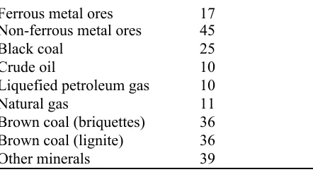
(37) Appendix 2: Database changes Table A2.1 shows the mineral supply elasticities implied by the ORANI-E database after the reallocation of mineral royalties from fixed capital to land. The elasticities are calculated using the formula in Dixon et al. (1982) p. 309. Table A2.2 shows emission intensities used in the database. These are defined as the ratio of a physical to a value unit, where the physical unit measures some quantity to be abated or conserved; in the present case, carbon dioxide emissions or energy content. The value unit is millions of 1986-87 dollars, valued at the point of production, excluding any excise or sales tax. The intensities are calculated using energy use statistics from the ABARE and input-output statistics from the ABS (Jones, Bush, Kanakaratnam, Leonard and Gillan 1991, ABS 1990a, b). Tables A2.3 and A2.4 provide a summary of the disaggregation of the electricity sector in the database. The disaggregation is based on electricity supply industry statistics from the Energy Supply Association of Australia Ltd, electricity generation cost estimates from Intelligent Energy Systems Pty Ltd, and published and unpublished ABARE estimates (ESAA 1993, IES 1991, Jones, Naughten et al. 1991). Table A2.1: Mineral supply elasticities Ferrous metal ores Non-ferrous metal ores Black coal Crude oil Liquefied petroleum gas Natural gas Brown coal (briquettes) Brown coal (lignite) Other minerals Source:. 17 45 25 10 10 11 36 36 39. ORANI-E database. Table A2.2: Emission intensities. Black coal Liquefied petroleum gas Natural gas Brown coal (briquettes) Brown coal (lignite) Petrol. and coal products Reticulated gas supply Sources:. Carbon dioxide (kt/$m) 76 9 33 101 134 8 9. Chemical potential energy (MJ/$m) 839 155 661 1062 1415 115 181. ABS (1990a, b), Jones, Bush et al. (1991). 33.

(38)

No results found