Monash University Wellington Road CLAYTON Vic 3168 AUSTRALIA Telephone:
(03) 9905 2398, (03) 9905 5112 from overseas:
61 3 9905 5112
Fax numbers: from overseas:
(03) 9905 2426, (03)9905 5486 61 3 9905 2426 or 61 3 9905 5486
e-mail [email protected]
Should Tariff Reductions be
Announced? An Intertemporal
Computable General
Equilibrium Analysis
by
Michael M
ALAKELLISCentre of Policy Studies/IMPACT Project
Monash University
Preliminary Working Paper No. OP-88 August 1997
ISSN 1 031 9034 ISBN 0 7326 0740 X
The Centre of Policy Studies (COPS) is a research centre at Monash University devoted to quantitative analysis of issues relevant to Australian economic policy. The Impact Project is a cooperative venture between the Australian Federal Government, Monash University and La Trobe University. COPS and Impact are operating as a single unit at Monash University with the task of constructing a new economy-wide policy model to be known as MONASH. This initiative is supported by the Industry Commission on behalf of the Commonwealth Government, and by several other sponsors. The views expressed herein do not necessarily represent those of any sponsor or government.
C
ENTRE
of
P
OLICY
S
TUDIES
and
the
I
MPACT
by
Michael MALAKELLIS
Centre of Policy Studies/IMPACT
Monash University
Abstract
In this paper the macro and structural implications of three alternative tariff-reduction strategies are examined. Under the first strategy, which is similar to that adopted in Australia in 1973, the tariff cut is implemented without warning. The second strategy is consistent with the current approach of phasing in tariff cuts according to a previously announced schedule. Under the third strategy the tariff cut is implemented several years after it is announced. We find that the long-run effects of the alternative tariff reduction strategies are similar, but that the adjustment paths are not. Our results suggest that if tariffs are to be reduced then it is preferable to implement the policy without warning. The results emphasise the point that the sooner tariffs are reduced the sooner will the allocative efficiency gains from doing so be realised.
Keywords: industry protection, tariffs, allocative efficiency,
com-parative-dynamic simulation, computable general equili-brium model, labour market adjustment, timing issues.
JEL classifications: D58, C68, E27, F13.
Communication to:
Michael Malakellis PO Box 7892
Waterfront Place BRISBANE
QLD 4001 Australia
E-mail: [email protected]
*
ii
Abstract i
I. Introduction 1
II. An Overview of ORANI-INT 2
(i) Treatment of Consumption 2
(ii) Treatment of Sectoral Investment 3
III. Simulating a Reduction in Assistance to Manufacturing 4
(i) Description of Experiments 4
(ii) Choice of Exogenous Variables 5
(iii) Control Scenario 6
IV. Simulation Results 6
(i) The Long-Run Results 11
(ii) The Transition Paths 16
(iii) Structural Adjustment 19
V. Summary and Conclusions 21
References 23
LIST OF FIGURES
Figure 3.1: Price of the Imported Manufacturing Commodity 5
Figure 3.2: Paths of Selected Real Macroeconomic Variables 7
Figure 3.3: Paths of Selected Price Deflators 8
Figure 3.4: Paths of Chief Export Commodities 9
Figure 3.5: Paths of Chief Imports 9
examine three approaches to reducing tariffs. Under the first approach, which is similar to that adopted in Australia in 1973, the tariff cut is implemented without warning. The second approach is consistent with the current practice of phasing-in tariff cuts according to a previously announced schedule. Under the third approach the tariff cut is implemented several years after it is announced.
There have been many studies of the effects of protection on the Australian economy. Surveys of this literature can be found in Lloyd (1978), Anderson and Garnaut (1987) and Powell and Snape (1993). The first CGE analysis was by Evans (1972). Since the late 1970s ORANI, a static CGE model (see Dixon, Parmenter, Sutton and Vincent, 1982), has been the dominant tool for assessing
Australia’s protection policies.1
Previous studies have provided estimates of how changes in protection affect regions, industries and occupations in either the short or long run. However, very little attention has been given to the adjustment path that the economy would take following a change in protection or to whether changes should be implemented without warning, as was done in 1973, or pre-announced and implemented gradually, as is the current practice.
The Jackson (1975) and Crawford (1979) reports favoured tariff reductions that were pre-announced and implemented in a series of small steps. In a review of The Jackson Report, Gregory (1976) argued that the recommended strategy ‘is not supported by in-depth analysis or evidence’. He suggested that it might be justified on adjustment assistance grounds but argued that pre-announced reforms might be less successful than unannounced reforms because the latter are more difficult to lobby against and reverse. The Jackson Report’s recommendation was also challenged by Gregory on the grounds that it might simply prolong the reform process. Gregory claimed that ‘tariff reform can proceed reasonably quickly with a tolerable level of adjustment costs’. This claim is based on calculations showing that the variations in the exchange rate experienced in the early 1970s placed greater pressure on industries to adjust than did the 25 per cent across-the-board tariff cut in 1973.2
Intertemporal CGE models like ORANI-INT are well suited to analysing alternative strategies for reducing protection. In contrast to static multisectoral models, ORANI-INT provides information about how a reduction in protection will change the structure of the economy over time. In addition, because ORANI-INT allows consumers and investors to be forward looking, the implications of announcing policy changes in advance of their implementation can be assessed.
The remainder of this paper is organised as follows. Section II provides a brief overview of ORANI-INT’s theoretical structure and database. Section III provides
1
ORANI has been used to analyse protection issues by government agencies, academics, lobby groups and businesses (see Powell and Snape, 1993). In part, the dominance of ORANI in industry protection analysis reflects the adoption of the model by the Industries Assistance Commission (succeeded in 1990 by the Industry Commission).
2
a description of how the tariff reductions are modelled. The simulation results are explained in section IV and concluding remarks are in section V.
II. An Overview of ORANI-INT
ORANI-INT (Malakellis, 1994) is a multi-period elaboration of ORANI. It consists of T identical single-period CGE submodels, each of which represents the economy at a different point in time. Each static CGE submodel is a modified version of ORANI that we call ORANI-13. The key differences between ORANI and ORANI-13 are that:
• ORANI-13 contains thirteen single-product sectors and recognises one type of
labour only, while ORANI distinguishes 112 sectors, 114 commodities and nine occupational groups;
• ORANI distinguishes between direct and margins demands for goods and
services3 whereas ORANI-13 does not; and
• ORANI-13 omits the ORANI equations that govern the sectoral distribution of
investment.
In ORANI and ORANI-13 aggregate investment and consumption are usually exogenous. In ORANI-INT the sequence of ORANI-13 submodels is linked through time via the specification of forward-looking investment and consumption behaviour. The forward-looking agents in the model are assumed to have model-consistent expectations.
The parameters used in ORANI-INT (e.g., export demand elasticities, expenditure elasticities, marginal budget shares, and elasticities of substitution between labour and capital and between domestic and foreign goods) are borrowed
from the ORANI parameter files.4
(i)Treatment of Consumption
The intertemporal consumption specification used in ORANI-INT is a discrete time elaboration of Lluch’s (1973) Extended Linear Expenditure System (ELES). The ELES uses an intertemporal utility function that is additively separable across time. The instantaneous utility function has the Klein-Rubin form. With this specification the representative household’s optimisation problem can be treated in two parts. First, the household must decide how to allocate lifetime disposable income (which in the absence of bequests is equivalent to lifetime expenditure) across time. Having decided its aggregate expenditure level in each period, the household must then decide how to distribute this expenditure among commodities. The former decision is intertemporal while the latter is atemporal.
The intertemporally optimising household in ORANI-INT distributes its consumption over time and over commodities to equalise the appropriately discounted marginal utility per dollar spent on all commodities in all periods.
3
Direct demands are those made by producers, investors, governments, households and foreigners. The satisfaction of direct demands generates demands for margins goods and services such as transport and wholesale and retail trade.
4
Given the Klein-Rubin form of the instantaneous utility functions, only a portion of each period’s expenditure is discretionary. With the behaviour of all households assumed to be identical, the equilibrium condition for the distribution of aggregate discretionary expenditure can be written as:
Dt
Dt+1 =
1+ρ 1 + it
Qt
Qt+1
Pt+1
Pt t=1...T-1 (1)
where D is aggregate discretionary consumption, ρ is the time preference rate, i is
the nominal interest rate, Q is the number of households and P is the discretionary-consumption price deflator. The present value of the discretionary-consumption stream is determined by the present value of household disposable income. Borrowing and lending by households are constrained by a terminal condition that requires the net-foreign-liabilities-to-GDP ratio to stabilise by the end of the planning period. An implication of (1) is that the growth rate of nominal per-household discretionary consumption will be zero if, as is assumed in the experiments reported in this
paper, it = ρ. The growth in real per-household discretionary consumption is
inversely related to the growth in prices.
(ii) Treatment of Sectoral Investment
Investment is done by producers. It involves the construction of sector-specific physical assets that yield diminishing streams of capital services. Sectoral investment is assumed to be irreversible. Financial markets are assumed to be competitive and the cost of funds is the rate of interest. A time-to-build investment specification with a one year gestation lag is assumed for all sectors. The representative producer/investor in the jth sector takes as given initial- and
terminal-period capital stocks,5 the path of output and the paths of all prices. The
production technology is exogenous to the producer/investor’s decision and CRS are assumed. The producer/investor chooses the paths of gross investment and factors of production (land, labour and capital) to minimise the present value of the expected future stream of costs.
The optimising producer/investor chooses the level of investment so that the imputed rental price (i.e., the marginal revenue product) of a unit of capital is equal to its marginal cost:
MRPKt+1 = θt[it + rt] + θt+1δ− [θt+1−θt] t=1...T-1 (2)
where MRPK is the marginal revenue product of capital, θ is the market valuation
of a unit of capital, r is an exogenous risk premium and δ is the rate of
depreciation.6 The marginal cost of capital is given by the three terms on the RHS
of (2). The first term is the opportunity cost of the capital-services-producing asset. Investment costs are incurred in year t for an asset that comes on stream in year
5
While terminal-period capital stocks are exogenous to the representative producer’s optimisation problem they are determined endogenously in ORANI-INT by a terminal condition that equates the growth in sectoral investment in the terminal period to that in the penultimate period.
6
t+1. The second term captures depreciation costs and the final term captures capital gains/losses. When the irreversibility constraint on investment is binding
(not binding), θ is less than (equal to) the construction cost of capital.
III. Simulating a Reduction in Assistance to Manufacturing
ORANI-INT is used to simulate the three alternative strategies for reducing tariffs on the Manufacturing commodity. The model is solved over a thirty year time horizon and results are reported as per-cent deviations from a control scenario.
(i) Description of Experiments
The tariff reductions are based on the Industry Commission’s (1995) estimates
of the nominal rate of assistance to Manufacturing between 1985-6 and 2000-1.7
The change in assistance to Manufacturing between 1985-6 and 2000-1 is modelled as a tariff movement that reduces the price of the imported
Manufacturing commodity by 8 per cent (i.e., [1.03 - 1.12]/1.12 = -0.08).8 In the first experiment the tariff cut is implemented fully in the first year of the planning horizon and is therefore unanticipated. In the second experiment the tariff cut is implemented in the 12th year of the planning horizon (notionally 1996-7) but is announced at the start of the planning horizon (notionally 1985-6). In the third experiment the tariff cut is phased in gradually over 12 years (notionally 1985-6 to
1996-7).9 The effects that the alternative tariff-cutting strategies have on the path
of the domestic currency price of the imported Manufacturing commodity are
shown in figure 3.1.10 The acronyms STR, ATR and PTR are used to describe the
Surprise Tariff Reduction, Anticipated Tariff Reduction and Phased Tariff Reduction experiments.
7
The IC estimates that the nominal rate of assistance to Manufacturing was 12 per cent in 1985-6 and will be 3 per cent 2000-1. These estimates include contributions by tariff and non-tariff measures, the latter accounting for less than 5 per cent of the measured assistance in 1992-3.
8
In the ORANI-INT database the tariff rate on the Manufacturing commodity is 0.084. Thus, to achieve the 8 per cent fall in the price of the imported Manufacturing commodity the tariff rate in ORANI-INT is reduced from 0.084 to -0.003 (a slight subsidy).
9
While the current schedule of tariff reductions extends to the year 2000-1, the cuts planned beyond 1996-7 are small (e.g., the nominal rate of assistance to the Manufacturing sector goes from 4 per cent in 1996-7 to 3 per cent in 2000-1). For convenience, we assume that the tariff reductions are completed by 1996-7.
10
-9.0 -8.0 -7.0 -6.0 -5.0 -4.0 -3.0 -2.0 -1.0 0.0
1 3 5 7 9 11 13 15 17 19 21 23 25 27 29
Percent Deviations from Control
Phased Tariff Reduction
Anticipated Tariff Reduction
Surprise Tariff Reduction
Year
Figure 3.1: Price of the Imported Manufacturing Commodity
(ii) Choice of Exogenous Variables
Since ORANI-INT has more variables than equations, some variables must be exogenously specified. The economic environment in which a particular experiment is analysed depends on the choice of exogenous variables.
The stock of capital available to each sector in year 1 is determined by investment undertaken in previous years. Hence, year 1 can be characterised as a short-run equilibrium in which sectoral capital stocks are held fixed and the sectoral rental prices of capital are free to vary. After year one sectoral capital stocks are free to vary while the rental prices are determined by equilibrium condition (2). Investment is endogenous in all periods. A terminal condition that requires the rate of growth of investment in the terminal year to be equal to that in the penultimate year is imposed.
The activities of two sectors, Public Administration and Community Services, are dominated by government expenditure. Investment in these sectors is assumed to be determined by government policy and is therefore exogenous in the tariff experiments.
Variables for which ORANI-INT has no theory are typically exogenous. These include technical and taste changes, indirect tax rates, risk factors, foreign demands, the foreign currency prices of imports, foreign interest rates, transfers overseas, population, government expenditure, the supply of agricultural land and exports of most commodities.
The supply side of the labour market is not modelled explicitly. Labour is assumed to be homogeneous and perfectly mobile. Aggregate employment is exogenous in all periods and the real wage adjusts to ensure that producers are on their labour demand schedules.
ORANI-INT is homogeneous of degree zero in prices. To determine the absolute price level a numeraire sequence is specified. The path of the nominal exchange rate plays this role.
(iii) Control Scenario
The control scenario is a balanced growth solution that satisfies all the non-linear equations of the model and in which all real variables grow by 3 per cent per annum (and all prices remain unchanged). The control scenario is based on a 13-sector aggregation of the 1980-1 ORANI database (corresponding with the ASIC divisions used by the ABS in the Australian National Accounts) configured to
exhibit balanced growth.11 Consistent with the length of the simulation horizon, the
control scenario extends over 30 years.
IV. Simulation Results
The simulation results are presented in figures 3.2 - 3.6. While the long-run effects of the alternative tariff reduction strategies are similar, the adjustment paths are not. Gains in real GDP and real aggregate consumption are greatest under the STR strategy and smallest under the ATR strategy. The tariff on the
Manufacturing commodity distorts the allocation of resources. The sooner the
distortion is reduced the sooner are the benefits of improved resource allocation realised.12
The tariff cut causes structural change. Structural adjustment problems will occur if the rate at which sectors must expand or contract exceeds their ability to
do so. In ORANI-INT the mobility of sectoral capital is constrained,13 limiting the
ability of sectors to expand or contract. Labour, however, is assumed to be homogeneous and perfectly mobile. These assumptions may be critical to the choice of tariff-reduction strategy.
In the following subsections the critical theoretical assumptions and critical elements of ORANI-INT’s database are used in explanations of the macro and sectoral results shown in figures 3.2 - 3.6. The long-run (i.e., year 30) results obtained in the three experiments are explained jointly because they are almost identical. The transition paths differ across simulations and, therefore, are explained separately. In subsection (iii) we indicate how much bigger the labour market adjustment costs must be under the ATR and PTR strategies relative to the STR strategy if the three strategies are to be equally preferred.
11
In configuring the ORANI database to exhibit balanced growth the sectoral net investment-capital ratios were adjusted to reflect 3 per cent growth in sectoral capital stocks.
12
In these experiments the removal of the distortionary tariff on the Manufacturing commodity is almost complete. While this improves real consumption in the long run, we do not claim that the optimal tariff is zero because Australia is assumed to have some market power in its export markets.
13
MR1: Real GDP MR2: Real Consumption (Sc=0.58)
-0.3 -0.2 -0.1 0.0 0.1 0.2 0.3 0.4 0.5 0.6 0.7
1 3 5 7 9 11 13 15 17 19 21 23 25 27 29
-0.90 -0.80 -0.70 -0.60 -0.50 -0.40 -0.30 -0.20 -0.10 0.00 0.10 0.20 0.30 0.40
1 3 5 7 9 11 13 15 17 19 21 23 25 27 29
MR3: Real Aggregate Investment (Si=0.25) MR4: Real Aggregate Capital Stock (Sk=0.29)
-15.0 -10.0 -5.0 0.0 5.0 10.0
1 3 5 7 9 11 13 15 17 19 21 23 25 27 29 -1.5 -1.0 -0.5 0.0 0.5 1.0 1.5 2.0
1 3 5 7 9 11 13 15 17 19 21 23 25 27 29
MR5: Aggregate Export Volumes (Se=0.17) MR6: Aggregate Import Volumes (Sm=0.17)
0.0 1.0 2.0 3.0 4.0 5.0 6.0 7.0
1 3 5 7 9 11 13 15 17 19 21 23 25 27 29 -10.0
-5.0 0.0 5.0 10.0 15.0 20.0
1 3 5 7 9 11 13 15 17 19 21 23 25 27 29
L e g e n d : S T R P T R A T R
Figure 3.2: Paths of Selected Real Macroeconomic Variables
PD1: GDP Deflator PD2: Investment Price Deflator -1.4 -1.2 -1.0 -0.8 -0.6 -0.4 -0.2 0.0
1 3 5 7 9 11 13 15 17 19 21 23 25 27 29
-2.0 -1.8 -1.6 -1.4 -1.2 -1.0 -0.8 -0.6 -0.4 -0.2 0.0
1 3 5 7 9 11 13 15 17 19 21 23 25 27 29
PD3: Export Price Deflator PD4: Factor Cost Deflator
-0.8 -0.7 -0.6 -0.5 -0.4 -0.3 -0.2 -0.1 0.0
1 3 5 7 9 11 13 15 17 19 21 23 25 27 29
-1.5 -1.0 -0.5 0.0 0.5 1.0 1.5
1 3 5 7 9 11 13 15 17 19 21 23 25 27 29
PD5: Rental Price of Capital Deflator PD6: Price of Labour
-2.0 -1.5 -1.0 -0.5 0.0 0.5 1.0 1.5 2.0 2.5
1 3 5 7 9 11 13 15 17 19 21 23 25 27 29 -2.5 -2.0 -1.5 -1.0 -0.5 0.0 0.5 1.0 1.5
1 3 5 7 9 11 13 15 17 19 21 23 25 27 29
PD7: Discretionary CPI PD8: CPI
-2.0 -1.5 -1.0 -0.5 0.0 0.5 1.0
1 3 5 7 9 11 13 15 17 19 21 23 25 27 29
-1.4 -1.2 -1.0 -0.8 -0.6 -0.4 -0.2 0.0 0.2 0.4
1 3 5 7 9 11 13 15 17 19 21 23 25 27 29
Legend: STR P TR A TR
Figure 3.3: Paths of Selected Price Deflators
CE1: Rural (Sr=0.19) CE2: Mining (Smin=0.16)
-3.0 -2.0 -1.0 0.0 1.0 2.0 3.0 4.0 5.0 6.0
1 3 5 7 9 11 13 15 17 19 21 23 25 27 29 -4.0 -2.0 0.0 2.0 4.0 6.0 8.0 10.0 12.0 14.0 16.0
1 3 5 7 9 11 13 15 17 19 21 23 25 27 29
CE3: Manufacturing (Sman=0.42)
0.0 1.0 2.0 3.0 4.0 5.0 6.0 7.0 8.0 9.0
1 3 5 7 9 11 13 15 17 19 21 23 25 27 29
Legend:
STR PTR ATR
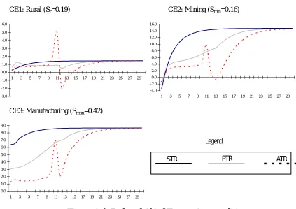
Figure 3.4: Paths of Chief Export Commodities
In the charts the values on the horizontal axis are years and the values on the vertical axis are per-cent deviations from the control solution. The Ss refer to shares in total exports.
CM1: Manufacturing (Sman=0.77) CM2: Mining (Smin=0.09)
-10.0 -5.0 0.0 5.0 10.0 15.0 20.0 25.0
1 3 5 7 9 11 13 15 17 19 21 23 25 27 29
-25.0 -20.0 -15.0 -10.0 -5.0 0.0 5.0 10.0
1 3 5 7 9 11 13 15 17 19 21 23 25 27 29
Legend: STR P TR A TR
Figure 3.5: Paths of Chief Imports
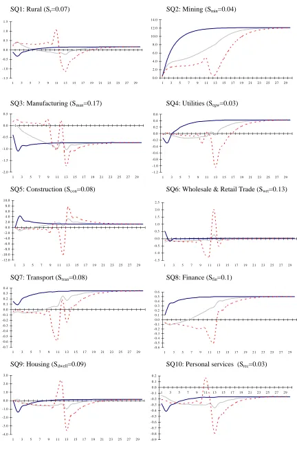
Figure 3.6: Sectoral Output Paths
In all charts the values on the horizontal axis are years and the values on the vertical axis are per-cent deviations from the control solution. The Ss denote shares in value added in the control solution.
-1.5 -1.0 -0.5 0.0 0.5 1.0
1 3 5 7 9 11 13 15 17 19 21 23 25 27 29 0.0 2.0 4.0 6.0 8.0 10.0 12.0
1 3 5 7 9 11 13 15 17 19 21 23 25 27 29
SQ3: Manufacturing (Sman=0.17) SQ4: Utilities (Segw=0.03)
-2.0 -1.5 -1.0 -0.5 0.0 0.5
1 3 5 7 9 11 13 15 17 19 21 23 25 27 29 -1.2 -1.0 -0.8 -0.6 -0.4 -0.2 0.0 0.2 0.4 0.6
1 3 5 7 9 11 13 15 17 19 21 23 25 27 29
SQ5: Construction (Scon=0.08) SQ6: Wholesale & Retail Trade (Swrt=0.13)
-12.0 -10.0 -8.0 -6.0 -4.0 -2.0 0.0 2.0 4.0 6.0 8.0 10.0
1 3 5 7 9 11 13 15 17 19 21 23 25 27 29 -1.5 -1.0 -0.5 0 .0 0 .5 1 .0 1 .5 2 .0 2 .5
1 3 5 7 9 1 1 1 3 1 5 1 7 1 9 2 1 2 3 2 5 2 7 2 9
SQ7: Transport (Stran=0.08) SQ8: Finance (Sfin=0.1)
-0.7 -0.6 -0.5 -0.4 -0.3 -0.2 -0.1 0.0 0.1 0.2 0.3 0.4
1 3 5 7 9 11 13 15 17 19 21 23 25 27 29 -0.6 -0.5 -0.4 -0.3 -0.2 -0.1 0 .0 0 .1 0 .2 0 .3 0 .4 0 .5 0 .6
1 3 5 7 9 1 1 1 3 1 5 1 7 1 9 2 1 2 3 2 5 2 7 2 9
SQ9: Housing (Sdwell=0.09) SQ10: Personal services (Srec=0.03)
-4.0 -3.0 -2.0 -1.0 0.0 1.0 2.0 3.0
1 3 5 7 9 11 13 15 17 19 21 23 25 27 29 -0.9 -0.8 -0.7 -0.6 -0.5 -0.4 -0.3 -0.2 -0.1 0.0 0.1 0.2
Legend : ST R P T R A T R
(i)The Long-Run Results
The long-run results of the three experiments are almost identical. This is because in all experiments the tariff has been cut to the same level after year 12 and the 30 year time horizon is sufficiently long for the economy to converge to its new long-run equilibrium. While the long-run results offer no basis for discriminating between the alternative tariff reduction strategies, an understanding of the mechanisms underlying these results is a prerequisite for understanding the adjustment paths. Investors and consumers are forward looking and the long-run results will influence the transitional dynamics.
We draw attention to the main mechanisms underlying the long-run results by explaining the following key results: the increase in real GDP; the increase in the economy’s capital-labour ratio; the small (relative to GDP) increase in real consumption; and the economy’s increased trade orientation. Having set the scene at the macro level we then turn to the sectoral results and explain why some sectors gain from the tariff cut while others lose.
Why does real GDP expand?
In ORANI-INT, GDP is measured in market prices. Indirect taxes put a wedge between the resource cost and market value of a unit of output. Changes in real GDP can be traced to changes in the usage of resources and/or to changes in the efficiency with which resources are used. From the income side, the percentage change in real GDP (rgdp) is defined as the weighted sum of the percentage changes in real value added (rva) and in real indirect tax revenues (rnit). That is:
rgdp=SGDP rvaVA +SGDP rnitNIT
, (3)
where SGDPVA and SGDPNIT are the shares in GDP of value added and net indirect
taxes. Chart MR1 shows that real GDP increases by about 0.64 per cent in the long
run. In the control scenario SGDPVA is 0.87 and SGDPNIT is 0.13.14 Using these
values as our estimates of the shares in (3)15 and using the year-30 simulation
results for rva and rnit the percentage change in real GDP can be decomposed as follows:
rgdp30 = 0 87 0 53. ( . )+0 13 1 36. ( . )= 0 64. .
Thus, about three quarters of the increase in real GDP emanates from the increase in real value added with the remainder being accounted for by the increase in real indirect tax revenues. Since capital is the only variable factor, the increase in real
14
Since the control scenario is configured to exhibit balanced growth, the values of the shares in equation (3), and in subsequent equations, are the same in all years.
15
value added in year 30 can be traced to the 1.61 per cent increase in the aggregate
capital stock (chart MR4).16
Net indirect taxes can change if the tax rates change and/or if the tax bases change. The tax bases can change through price or quantity movements. The model distinguishes production taxes by sector, sales taxes by user (i.e., producers, investors, households, governments, and foreigners) and tariffs. The corresponding bases are the basic values of outputs, the basic values of sales of commodities (domestic and foreign) and the cif values of imports. We define rnit as that part of the percentage change in net indirect taxes that is due to changes in the tax bases caused by changes in quantities. That is:
rnit SNIT zj SNIT x SNIT x
p j
j i r s r
i
i r i t i
i
= + +
= = = =
∑
∑
∑
∑
1 13
1 2
1 13
2 1
13
2
, , , , . (4)
In (4) the indices j, i and r refer to industries, commodities and sources (i.e., r=1
denotes domestic source and r=2 denotes foreign source). SNITk , k∈{p,s,t}, is the
share in aggregate net indirect tax revenues of tax of type k (production tax, sales tax or tariff) collected from the production or sale of commodity i. The lower-case
variables z and x denote the percentage changes in outputs and sales.17
In the absence of any changes in the composition of sectoral outputs and sales, the zs and xs in (4) will move together. Under these conditions rnit, and therefore rgdp [via (3)], will be equal to rva (which is the weighted sum of the zs). However, the tariff shock induces a change in the economy’s production and sales structures in favour of commodities that are relatively highly taxed. This compositional change causes rnit and, therefore, rgdp to exceed rva. The excess of rgdp over rva represents the allocative efficiency gains from changing the composition of the economy in favour of activities that were discouraged (relative to optimum) in the pre-shock tax regime. Most of the excess of rnit over rva can be attributed to: a 12 per cent expansion in the Mining sector’s output, which is heavily taxed; a 0.73 per cent contraction in the Manufacturing sector’s output, which is relatively lightly
taxed; a 1.4 per cent increase in sales of the Manufacturing commodity18 which
attract a relatively high rate of tax; and a 9.9 per cent increase in the volume of the imported Manufacturing commodity which attracts the highest tariff.
Why does the economy become more capital intensive?
Most of the increase in the economy’s capital is accounted for by the fall in the user cost of capital (i.e., by the fall in the rental price of capital relative to the price of other factors). By year 30 the economy has converged to its new steady state in which there are no capital gains/losses. This means that the rental price of capital
and the construction cost of capital will move together.19 In year 30 the
16
The share of capital in value added is 0.33. Hence, rva30 = 0.33(1.61) = 0.53. 17
The sales tax rates in ORANI-INT differ across users. To keep our presentation simple, we have not represented these differences in equation (4).
18
Sales of the Manufacturing commodity increase because the 9.9 per cent increase in imports of the Manufacturing commodity outweighs the 0.73 per cent decrease in sales of the domestic variety.
19
This can be deduced from equilibrium condition (2). In the steady state θt+1 = θt. Under these
conditions (2) reduces to: MRPKss = θss[iss + rss + δ]. Since the variables i, r and δ are held constant,
reducing effect of the tariff cut allows the average construction cost of capital, measured by the investment deflator, to fall by about 1.8 per cent (chart PD2). This translates into a 1.64 per cent fall in the average rental price of capital (chart
PD5).20 In contrast, the value-added deflator, which indicates the average cost of
all primary factors, rises by about 0.1 per cent (chart PD4).
The investment deflator falls by more than the GNE deflator (1.13 per cent compared with 1.8 per cent) because the capital creation process is relatively intensive in the use of the imported Manufacturing commodity whose price falls by 8 per cent. In turn, the GNE deflator falls relative to the value-added deflator which is the GDP deflator net of indirect taxes. In these experiments there are two counteracting mechanisms that allow the value-added deflator to move out of line with the GNE deflator. The tariff cut tends to reduce the real cost of capital by allowing the value-added deflator to rise relative to the GNE deflator. The tariff cut improves Australia’s competitiveness and encourages an expansion in exports. This induces a deterioration in the terms of trade which tends to increase the cost of using capital by allowing the value-added deflator to fall relative to the GNE deflator. However, the terms of trade deterioration only partially offsets the fall in the user cost of capital induced by the tariff cut.
Why does the economy become more trade oriented?
In these simulations the foreign interest rate is 3 per cent and the steady-state rate of growth of real variables is assumed to be 3 per cent. Therefore, in the
steady state, net foreign liabilities (NFL) accumulate passively21 at 3 per cent and
GDP grows at 3 per cent. For the economy to enter year 30 with a stable NFL-to-GDP ratio, the trade deficit in year 30 must be zero (i.e., no active accumulation of foreign liabilities is allowed). Thus, the stimulus given to imports by the tariff reduction must be offset by an expansion in exports. In the three simulations reported, the nominal exchange rate and the foreign currency price of imports are assumed to remain at their control scenario values in all years. Therefore, in year 30 the foreign currency value of exports increases at the same rate (5.6 per cent) as
the volume of imports (chart MR6).22
The increase in imports shown in chart MR6 is accounted for by the 9.9 per cent increase in imports of the Manufacturing commodity (chart CM1) and by the 23 per cent fall in imports of the Mining commodity (chart CM2). In the control scenario the Manufacturing commodity accounts for 77 per cent of total imports hence its contribution to the increase in aggregate imports is about 7.6 percentage
points (0.77×9.9). Imports of the Mining commodity, which account for 0.09 per
cent of total imports, contribute -2.07 percentage points (0.09×(-23)).
20
The simulation results for year 30 show that for each sector the percentage change in the rental price of capital is equal to the percentage change in the construction cost of capital. The discrepancy in year 30 between the percentage change in the average rental price of capital and the percentage change in the average construction cost of capital is accounted for by aggregation effects. The weights used to construct the two price indexes are different.
21
By passive accumulation of net foreign liabilities we mean additions/reductions to net foreign liabilities arising from interest charges/receipts on the existing stock of net foreign liabilities.
22
The fall in the price of the imported Manufacturing commodity induces competing effects on the trade balance. The expansion in imports of the
Manufacturing commodity tends to worsen the trade balance but this is
counteracted by the improvement in competitiveness which encourages import replacement as well as export sales. The imported Manufacturing commodity is an important input into capital creation and current production (accounting for about 10 per cent of total intermediate usage and about 11 per cent of total inputs into capital creation) hence the fall in its price tends to reduce domestic costs and improve competitiveness.
The purchasers’ prices of imports other than Manufacturing remain unchanged and the fall in domestic costs tends to reduce the demand for these imports. For example, the fall in domestic costs is particularly harmful to Mining imports because the domestic and foreign Mining commodities are assumed to be close substitutes (the Armington elasticity for this commodity is 36 reflecting mainly the tradeability of Oil). The demands by foreigners for the Rural, Mining and
Manufacturing commodities are cost sensitive and, as figure 3.4 shows, exports of
these three commodities increase.
Why is the increase in real consumption small relative to the increase in real GDP?
The expansion in the economy’s capital stock and the allocative efficiency gains induced by the tariff cut allow real GDP to expand by 0.64 per cent. However, not all of this increase is available to Australian households. The contribution made to real GDP by the expansion in capital stocks will be offset by the investment expenditure required to maintain the capital stock at its new higher level. In addition, because the tariff cut induces a deterioration in Australia’s terms of trade some of the increase in real GDP accrues to foreigners.
Given that the trade account must be balanced in year 30, the deterioration in the terms of trade means that any increase in the volume of imports must be more than offset by an increase in export volumes. In the control scenario, which has balanced trade in all years, the shares of exports and imports in GDP are 0.17. Export volumes increase by 6.3 per cent in year 30 (chart MR5) but, because the terms of trade deteriorate, balanced trade is maintained with an increase in imports of 5.6 per cent only. Thus, about 0.13 percentage points (i.e., 0.17(6.31) -0.17(5.56)) of the 0.64 per cent increase in real GDP is not available for domestic absorption. The share of investment in GDP is 0.25 and the 1.8 per cent increase in aggregate investment absorbs about 0.45 percentage points (i.e., 0.25(1.8)) of the increase in real GDP. Only the residual increase in real GDP (i.e., about 0.06 percentage points) goes to private consumption.
Sectoral results
Other things constant, the tariff cut favours capital intensive industries by allowing the price of labour to rise relative to the price of capital (compare charts PD5 and PD6). Since the profitability of supplying capital is exogenous, the gains from the tariff cut (i.e., the allocative efficiency gains less the terms of trade losses) accrue to labour which is the fixed factor.
about 25 per cent of the sector’s total costs and it gains a competitive advantage from the fall in the price of capital. The Mining sector gets an additional cost advantage from the fall in the price of the Manufacturing commodity which accounts for about 30 per cent of its intermediate inputs. This improvement in competitiveness allows the Mining sector to expand its exports by almost 15 per cent (chart CE2) as well as to gain market share from the imported Mining commodity (chart CM2).
Compared to Mining the improvement in the Rural sector’s competitiveness is modest. This is reflected by the smaller expansion in its export sales (chart CE1). The Rural sector is an intensive user of the Manufacturing commodity (both domestic and foreign) and benefits from the fall in the price of this input. This is mitigated by increases in the prices of labour and agricultural land which account for over half of the Rural sectors total costs (i.e., 35 and 20 per cent respectively). The supply of agricultural land is fixed and its price rises as the Rural sector expands. The increase in the sector’s output is modest because the increase in its export sales is small (about 1.5 per cent) and because its main domestic customer, the Manufacturing sector, contracts.
The Manufacturing sector contracts because the tariff cut improves the competitiveness of the foreign Manufacturing commodity. This sector is relatively labour intensive and its competitiveness is reduced further by the increase in wages. The loss of competitiveness is partially offset by the 8 per cent fall in the price of the imported Manufacturing commodity, which accounts for about 12 per cent of the sector’s intermediate inputs, and by the fall in the cost of capital. While
Manufacturing is not very capital intensive, the 2.6 per cent fall in the price of its
capital is the largest recorded for any sector. This is because Manufacturing’s capital creation process is the most intensive user of the imported Manufacturing commodity. The cost reductions in the Manufacturing sector are reflected by the 8.7 per cent expansion in its export sales. However, its output falls by about 0.7 per cent because the expansion in exports is more than offset by the loss of domestic sales to the cheaper imported Manufacturing commodity (chart CM1).
The increase in real consumption is small and is of little benefit to most domestic industries. The allocation of the household budget depends on the relative prices of consumer goods. The fall in the price of the imported
Manufacturing commodity induces households to reallocate their budget in its
favour. Two domestic commodities, Utilities and Housing, also capture a slightly larger share of the household budget. These sectors are relatively capital intensive and the fall in the cost of capital allows the price of their output to fall relative to the prices of other consumer goods. While the Utilities sector benefits from the increase in sales to households, most of the 0.42 per cent increase in its output is accounted for by the increase in sales to intermediate users, in particular to the
Finance and Housing sectors.
The Personal services sector sells about 70 per cent of its output to households yet chart SQ10 shows its output falls despite the increase in aggregate consumption. This is because its production structure is labour intensive and the fall in its costs relatively small. For similar reasons, sales by the Wholesale and
Retail Trade (WRT) sector to households fall. The WRT sector records a modest
The Construction sector’s fortunes are closely related to investment activity, which increases. The expansion in Housing is important because that sector purchases about 30 per cent of Construction’s output. Capital is the only factor of production used by Housing and its capital and output increase by the same proportion. The domestic Construction commodity accounts for almost all of the inputs to Housing’s capital creation process. The Housing sector owns about 30 per cent of the economy’s capital stock hence the small increase in its output generates a significant increase in the demand for the Construction commodity.
The expansion in the Transport and Finance sectors is related to the increase in the demand for their outputs by the Mining and Construction sectors.
(ii) The Transition Paths
Since the long-run results obtained in the three experiments are almost identical, the assessment of the relative merits of the alternative tariff reduction strategies must be based on differences in the transition paths. The adjustment to the long-run equilibrium is slowest in the ATR experiment and fastest in the STR experiment. For example, in the STR experiment real GDP completes about 85 per cent of the adjustment to its long-run value in 5 years. The same adjustment takes about 20 years in the ATR experiment and 15 years in the PTR experiment.
Below we explain why the economy adjusts more slowly in the PTR and ATR experiments than in the STR experiment. We also point out that the volatility evident in the adjustment paths is related to the behaviour of investors rather than consumers.
Speed of adjustment in real GDP
In the explanation of the long-run results we related changes in real GDP to changes in capital stocks and to changes in allocative efficiency. This relationship applies in all years. Capital accounts for about 30 per cent of GDP and it is evident from charts MR1 and MR4 that in most years the change in capital stocks explains
most of the change in real GDP.23
In the three experiments capital stocks are unable to adjust in the first year. Thereafter, changes in capital stocks are closely related to changes in the real cost of using capital. Other things constant, the cut in the tariff on the Manufacturing commodity allows the real cost of using capital to fall. Beyond year 1 rates of return on all assets are assumed to be equal. In maintaining this asset market equilibrium, agents investing in fixed capital trade off increases/decreases in rentals with capital losses/gains. It is cheaper for producers to expand their capital
23
stocks gradually, rather than abruptly, because rapid expansion in investment in year t generates capital losses in that year which are traded off for higher rentals in year t+1. However, the higher rentals in year t+1 discourage the use of capital by producers in that year tending to dampen the investment response in year t.
In the STR experiment the tariff cut is implemented fully in year 1 and hence has the same direct effect on the cost of capital (i.e., from the availability of cheaper imports) in all years. However, the reductions in the cost of capital emanating indirectly from the tariff cut become progressively more pronounced after year 1 as the economy’s supply constraints become progressively less severe. Accordingly, producers delay their investment decisions because they anticipate (correctly) that investment costs will fall in the future.
In the PTR experiment agents do not anticipate the tariff cut implemented in year 1, but anticipate the subsequent tariff cuts. Despite knowing about the impending tariff cuts they react more slowly than in the STR experiment. Forward-looking investors delay their investments in anticipation of further falls in the cost of creating capital. The direct effect of the tariff cut on the cost of capital gets bigger in line with the phasing in of the tariff cut whereas in the STR experiment the direct effect is the same in all years.
The distinguishing feature of the capital path obtained in the ATR experiment is that it falls below control in the lead up to the tariff cut in year 12. The reason for this is that producers allow their capital stocks to fall (by delaying their investments) to avoid anticipated capital losses in year 12. The reduction in capital stocks between years 2 and 12 is gradual because it is cheaper to reduce capital stocks gradually rather than abruptly. Over this period capital losses get progressively bigger and the rental price of capital rises. Beyond year 12 the capital losses get smaller and the rental price of capital falls gradually. This is reflected in the gradual increase in capital stocks after year 12. The capital losses fade away after year 12 because there are no further reductions in the cost of capital emanating directly from the tariff cut and because the economy’s supply constraints become progressively less severe.
Behaviour of consumers
Under the Klein-Rubin utility function, real consumption is made up of subsistence and discretionary consumption. Since real subsistence consumption (per-capita) is assumed to remain unchanged over time, it is possible to explain the path of real aggregate consumption with reference to the path of real discretionary expenditure only.
The consumption specification in ORANI-INT and the closure adopted for these experiments implies that the proportional change in nominal discretionary
expenditure will be the same in all years.24 Moreover, because the results obtained
in the three experiments converge in the long run, the path of nominal discretionary expenditure will be the same in the three experiments. However,
24
because the proportional deviations in consumer prices may be different over time, the proportional deviations in real discretionary expenditure need not be the same in all years. Households will bias their discretionary consumption in favour of the years in which prices are relatively low (and vice versa).
The consumption paths depicted in chart MR2 mirror the CPI paths shown in
chart PD8.25 In all three experiments households tend to bias their consumption in
favour of the later years because consumer prices are lower in the later years relative to the early years. In all experiments the cost reductions emanating directly and indirectly from the tariff cut become progressively more pronounced as the economy’s supply constraints become less severe. In the STR experiment the direct cost reductions are the same in all years and the economy’s productive capacity is expanded gradually after year 2. In the PTR experiment the direct cost reductions increase gradually with the phasing in of the tariff cut. This delays the expansion of the economy’s productive capacity. The cost-reducing effects of the tariff cut are delayed further in the ATR experiment because the policy is not implemented until year 12.
The non-monotonicity of the CPI paths, and consequently the consumption paths, can be traced to the volatility of the price of Housing which has a large weight in the consumption basket (about 20 per cent). A special feature of the
Housing sector is that capital is the only primary-factor input that it uses. Since
capital accounts for over 70 per cent of Housing’s total costs, the price of Housing services is closely related to the cost of the sector’s capital stock.
In the first year of the simulations sectoral capital stocks are assumed to be unaffected by the tariff shock and the rental price of capital adjusts to clear the capital markets. In subsequent years capital stocks are free to vary but the rental price of capital is constrained by equilibrium condition (2). Thus, beyond year 1 the rental price of the Housing sector’s capital is constrained to reflect investment costs and capital gains/losses.
The effect on real consumption of holding Housing’s capital stock at its control scenario level in year 1 is most evident in the STR experiment where the tariff cut is fully implemented in year 1. Contrary to our expectations the path of prices does not fall gradually over time as the economy adjusts its productive capacity to the new long-run equilibrium level. Chart PD7 shows that the CPI falls sharply in year 1 relative to year 2 and this is reflected in chart MR2 by the modest fall in real consumption in year 1 relative to year 2. The sharp fall in the CPI in year 1 is caused by the fall in the price of Housing in that year.
The expenditure elasticity for Housing services is high (1.34). Hence, the 0.9 per cent reduction in nominal discretionary expenditure causes the demand for these services to fall relatively strongly. Since the supply of Housing services cannot change in year 1, the price of these services falls to accommodate the fall in demand. In year 1 the decrease in the price of Housing is absorbed by a fall in the rental price of the Housing sector’s capital stock.
Beyond year 1 the rental cost of the Housing’s capital depends on investment costs and on the rate of change in investment costs (i.e., capital gains/losses). The
25
Construction sector supplies about 95 per cent of the inputs to Housing’s capital
creation process. Thus, the rental price of Housing’s capital stock will reflect the price of the Construction commodity and its rate of change over time. The
Construction sector is an intensive user of the Manufacturing commodity
(domestic and imported) and sells most of its output to capital creators. Therefore, the price of the Construction commodity and its rate of change over time depends on the size and timing of the tariff cuts and on the size and timing of the aggregate investment response.
The link between the price of the Construction commodity, the cost of
Housing’s capital and real aggregate consumption is most evident in the ATR
experiment for the three years centred around year 12 the year in which the
tariff cut is implemented. Although not reported, the rate of growth in price of the
Construction commodity between years 11 and 12 is positive. Over this period the
tariff cut causes the rate of growth in the price of the Construction commodity to fall but this effect is more than offset by the increase in the rate of growth in the price of the Construction commodity caused by the turn-around in aggregate investment between years 11 and 12 (see chart MR3). In year 11 the sharp decrease in aggregate investment causes the price of the Construction commodity to fall below control while the sharp increase in aggregate investment in year 12 has the opposite effect. This pattern in the price of the Construction commodity generates capital gains for the Housing sector in year 12. These gains allow the rental cost of the Housing sector’s capital stock, and consequently the price of the
Housing commodity, to fall below control in year 12. In year 12 the fall in the price
of Housing causes the CPI to fall and real consumption to rise.
Note that the increase in real consumption in year 11 is similar to that in year 12 because the fall in the CPI in those two years is similar. Despite the fact that rate of growth in aggregate investment between years 10 and 11 is declining, the rate of growth of investment by the Construction sector increases sharply over this period. This is because the Construction sector expands its capacity in anticipation of the aggregate investment surge in year 12. The price of the Housing commodity falls in year 11 because the capital gains generated by the growth in investment by the
Construction sector allow Housing’s capital costs to fall.
In year 13 the CPI rises above control causing real consumption to fall below control. This is largely due to the capital losses generated by the fall in the rate of growth of aggregate investment between years 12 and 13. Beyond year 13 the rate of growth of aggregate investment falls at a decreasing rate. Thus the capital losses get progressively weaker over time and as shown in chart MR2 the path of real consumption rises gradually after year 13.
(iii) Structural Adjustment
Over the 30 year simulation horizon26 the present value of the consumption
stream increases by 0.065 per cent in the STR experiment, falls by 0.032 per cent in the PTR experiment and falls by 0.128 per cent in the ATR experiment. Year 1 of the simulation is assumed to represent 1985-6. Nominal consumption in that year was $143,791 million. Thus, relative to the control scenario the change in the
26
present value of consumption, in millions of 1985-6 dollars, is $2804 (i.e., 30×
0.00065×$143,791) in the STR experiment and -$1394.77 and -$5521.57 in the
PTR and ATR experiments.
Before drawing policy conclusions from the above results, the implications that the alternative tariff reduction strategies have for labour market adjustment costs must be considered. The costs of moving workers have not been explicitly modelled. Labour is assumed to be homogeneous and perfectly mobile between sectors and real wages are assumed to adjust to ensure that aggregate employment is unaffected by the tariff cut. Labour market adjustment costs are likely to be greater when structural change is rapid. Since the STR strategy causes the economy to adjust more rapidly than do the PTR and ATR strategies, it is possible that the former strategy gives rise to greater labour market adjustment costs.
An indication of how sensitive our conclusions are to the labour market assumptions can be obtained by estimating the extent to which labour market adjustment costs might differ in the three experiments and relating these differences to the corresponding consumption gains/losses. We assume that labour market adjustment costs are related to the number of workers that must change occupation. For each experiment the employment results for the 13 ORANI-INT
sectors are mapped to the 52 ASCO minor group occupational categories.27 From
the occupational employment results we infer the number of workers who must change occupation in each of the three experiments.
To estimate the number of workers who must change their occupation we make two simplifying assumptions: first, workers change occupation only if there is a decline in employment in occupation o between years t and t+1; and, second, all
workers that change occupation obtain another job28. Under these assumptions, the
number of workers that move from occupation o in year t to some other occupation in year t+1 is equal to the bigger of the following two numbers: zero and the
difference between employment in occupation o in years t and t+1 (i.e., Lo,t - Lo,t+1).
By summing over occupations and time we obtain the total number of workers that
change occupation over the simulation horizon, LM, as follows:
(
)
{
}
LM Lo t Lo t
t
= − +
=
=
∑
∑
max , , 1 ,0 1 52
1 29
0 (5)
Applying (5) to the occupational results we detect occupational changes in the ATR simulation only. The number of workers that must change occupation in the ATR simulation is equivalent to 0.21 per cent of the control scenario level of
employment in year 1.29 The tentative conclusion that can be drawn from the
occupational results is that there is little evidence of substantial labour market adjustment costs arising from the tariff cuts examined. Our analysis suggests that, whether the objective is maximising real consumption or minimising worker
27
To do this mapping we use shares derived from 1994-5 industry-by-occupation employment data.
28
A more detailed analysis of labour market adjustment costs would allow for retrenched workers to move into unemployment (permanently or temporarily) and for some of the new jobs generated by the tariff shock to go to persons that were previously unemployed.
29
displacement, the STR strategy dominates (or is equivalent to) the PTR strategy which, in turn, dominates the ATR strategy.
Although our assessment of labour market adjustment costs is instructive, it has several limitations and the results should be interpreted with caution. One problem is that we use an unrealistic control scenario. Of particular relevance to the issue of labour market adjustment costs is the assumption in the control scenario that employment in each occupation grows by 3 per cent per annum. In the three tariff-cut experiments the growth in employment in the different occupations is allowed to deviate from 3 per cent in response to the shock but aggregate employment is assumed to remain on its control scenario path. This means that there will be a redistribution of employment opportunities away from those occupations heavily exposed to industries adversely affected by the tariff cuts (e.g., trades assistants
and factory hands about 66 per cent of which are employed in the Manufacturing
sector) towards occupations exposed to industries that benefit from the policy change (e.g., construction and mining labourers about 53 per cent of which are employed in the Construction sector). While our results confirm this pattern in the redistribution of employment opportunities they also indicate that in the STR and PTR experiments the changes in the structure of the economy induced by the tariff shocks are not big enough to cause employment growth in any occupation to be
negative.30 Our estimate of labour market adjustment costs is sensitive to the
growth rates of employment in the 52 occupations assumed in the control scenario. For example, our estimates of the number of workers that change occupation in response to the tariff cuts will be understated if we have overstated the employment prospects of trades assistants and factory hands in the control scenario.
Our measure of labour market adjustment costs is also sensitive to the level of aggregation. We have identified 52 occupational groups and movements of workers within these groups are ignored. Moreover, our calculations ignore a range of potentially important adjustment costs. For example, we do not take into account the costs of moving workers between industries and regions. Potentially, the most significant adjustment costs not captured in the simulations are those associated with unemployment. We have assumed that real wages adjust to ensure that aggregate employment is unaffected by the tariff shocks. At least in the short run, it is probable that real wage rigidities exist for some occupations. Under such conditions the tariff shocks may induce changes in the rate of unemployment in
particular occupational categories and in aggregate.31
V. Summary and Conclusions
The results presented in this paper suggest that the long-run effects of a tariff cut are independent of the way in which the policy is implemented. The three tariff
30
In the ATR experiment the changes in the structure of the economy around year 12 (when the tariff shock is implemented) are sufficiently large to cause the rate of growth in employment of construction and mining labourers and building tradespersons to fall in year 11.
31
reduction strategies considered generate similar increases in real GDP and real consumption in the long run. The long-run increase in real GDP is related mainly to the expansion of the capital stock. The capital creation process is intensive in the use of the imported Manufacturing commodity and the cut in the tariff on this commodity allows the real cost of using capital to fall. The NFL-to-GDP ratio is assumed to stabilise in the long run and this means that the trade balance cannot be affected by the tariff shock in the long run. In the long run, therefore, the expansion in imports that is induced by the tariff cut must be matched by an expansion in exports. Since Australia is assumed to have some market power in its export markets, the increase in exports is accompanied by a decline in the terms of trade. The decline in the terms of trade is borne mainly by private consumers and as a result the increase in real consumption is modest.
The effects of the tariff cut in the short and medium run are sensitive to the way in which the shock is implemented. On the basis of the path of either real GDP or real consumption, the results indicate that an unannounced tariff reduction is preferable to an announced, gradual tariff cut which in turn is preferable to an anticipated tariff reduction. Real GDP is higher in all periods in the case where the tariff cut is implemented without warning. Over the 30 year simulation horizon the present value of the consumption stream increases by 0.065 per cent under the STR strategy and falls by 0.032 and 0.128 per cent under the PTR and ATR strategies. Under the latter two strategies Australians forego some of the benefits that can be derived from the availability of cheaper imports.
References
Anderson, K. and R.G. Garnaut (1987) Australian Protectionism: Extent, Causes
and Effects, Sydney: Allen and Unwin.
Dixon, P.B., B.R. Parmenter, J. Sutton and D.P. Vincent (1982) ORANI: A
Multisectoral Model of the Australian Economy, North-Holland,
Amsterdam.
Evans, H.D. (1972) A General Equilibrium Analysis of Protection: The Effects of Protection in Australia, North-Holland, Amsterdam.
Gregory, R.G., (1976) “The Green Paper on Policies for Manufacturing Industry: A Review”, Australian Journal of Management, Vol. 1, pp. 51-75.
Gruen, F.H., (1975) “The 25% Tariff Cut, was it a mistake?”, The Australian
Quarterly, 47(2), pp. 7-20.
Industry Commission (1995) Assistance to Agricultural and Manufacturing Industries, Information Paper, March, Australian Government Publishing Service, Canberra.
Lloyd, P.J., (1978) “Protection Policy”, chapter 5 in F.H. Gruen (ed.) Surveys of
Australian Economics, Vol. 1, Sydney: George Allen and Unwin.
Lluch, C., (1973) “The Extended Linear Expenditure System”, European
Economic Review, Vol. 4, pp. 21-32.
Lucas, R.E., (1967) “Adjustment Costs and the Theory of Supply”, Journal of
Political Economy, Vol. 75, pp. 321-334.
Malakellis, M. (1994) “ORANI-INT: An Intertemporal Computable General Equilibrium Model of the Australian Economy, Unpublished Ph.D Thesis, Monash University.
Powell, A.A. and R.H. Snape (1993) “The Contribution of Applied General Equilibrium Analysis to Policy Reform in Australia”, Journal of Policy
Modeling, 15(4), pp. 393-414.
The Crawford Report (1979) Commonwealth of Australia, Study Group on
Structural Adjustment Report, Australian Government Publishing Service,
Canberra.