A Survey of Image Compression using Neural Network and Wavelet
Transformation
Rajkishore Yadav
1; R. K. Gupta
2& A. P. Singh
3 Department of Computer Science and Engineering Azad Institute of Engineering and Technology, Lucknow, India[email protected], [email protected]2, [email protected]3
ABSTRACT
Image compression is one of most extensively addressed research area. There are so many technologies are already existing on image compression such as JPEG, MPEG and H.26x standards apart from this some new technologies such as neural network and wavelet transformation have been developed to investigate the bright future of coding for image compression. This paper deals with the area of image compression as its application to various image processing fields. Extensive surveys on the development of neural network and wavelet transformation for image compression have been presented in this paper. In this research paper, we also explain the various error metrics like Data Compression Transformation, Mean Square Error (MSE) and Peak Signal to Noise Ratio (PSNR).
Key words-
Image compression; neural network; wavelet transformation; MSE; PSNR
1. INTRODUCTION
The fast development of computer applications came with high increase of the use of digital images, especially in the area of multimedia, games, satellite transmissions and medical imagery. Digital form of the information secures the transmission and provides its manipulation. Constant increase of digital information quantities needs more storage space and wider transmission lines. This implies more the research on effective compression techniques. The basic idea of image compression is the reduction of the middle number of bits by pixel (bbp) necessary for image representation.
The recent growth of data intensive multimedia-based web applications have not only sustained the need for more efficient ways to encode signals and images but have made compression of such signals central to storage and communication technology.
Image compression is the technique which reduces the amount of data required to represent a digital image. The basis of the reduction process is the removal of redundant data. From a mathematical point of view, this amounts to transforming a 2-D pixel array into a statistically uncorrelated data set. The transformation is applied before, storage or transmission of the image. A large amount of data is generated when a 2-D intensity function is sampled and quantized to create an image which is digital in nature. The amount of data generated results in impractical storage, processing and communication requirements. Image compression addresses such problems by reduction of the amount of data necessary to represent a digital image.
An effective image compression algorithm is proposed by introducing the artificial neural network (ANN) on the place of quantization block of a general image compression algorithm. In this method, after the spatial information of the target image is transformed in to the equivalent frequency domain, the ANN stores each of the transformed coefficients in the networks synaptic weights.
2. NEURAL NETWORKS
Neural Network [2] designs can be single layered only with the output layer or multi-layered with one or more hidden layers. A neural network can be deterministic where the impulses to the other neurons are sent when a neuron gets to a certain activation level and another is stochastic where impulses to the other neurons are sent by a probabilistic distribution. A neural network can also be a static network where the inputs are received in a single pass and dynamic network where the inputs are received over a time interval.
2.1 DIFFERENT NEURAL NETWORKS
The first modeling of a neuron was achieved by McCulloch and Pitts. Being inspired by the biologic neurons, they proposed the following model:
Figure 1: McCulloch and Pitts Model
In figure 1, a formal neuron receives a number of inputs (x1, x2,……xn); a weight
(w1, w2,….. wn) representative of the strength of
the connection is associated with each of these inputs. The neuron makes the weighted sum of its inputs and calculates its outputs by a non linear transformation of this sum.
There are different types of neural networks, among which we can mention two categories known as supervised network and unsupervised network.
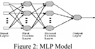
The model of the Multi - Layer perceptron [2] known a supervised network because it requires training to provide the desired output (target). The input data are repeatedly presented to the neural network. For every presentation, the output of the network is compared to the target and an error is calculated. This error is then used to adjust the weights so that the error decreases with every iteration and the model becomes closer and closer to the reproduction of the target.
Figure 2: MLP Model
Figure 2 shows the generalized structure of MLP model, it comprises basically three layers the input layer, hidden layer and one output layer. The number of hidden layers can be increased as per need for the appropriate network structure.
The radial basis function networks possess three layers and form a particular class of the Multi Layers networks .Every neuron of the hidden layer uses a core function called kernel function (for example, the Gaussian) as function of activation. This function is centered around the specified point by the weight vector associated with the neuron. The position and the „‟width‟‟ of these curves are learned from the bosses.
Figure 3: RBF Neural Network
In above figure 3, structure of radial basis function network shown. In general, there are fewer core functions in the RBF network than in inputs. Every neuron of the output implements a linear combination of these functions; the idea is to approximate a function by a set of other ones. From that point of view the hidden neurons provide a set of functions that form a basis representing the inputs in the “covered space” by the hidden neurons.
3. WAVELET TRANSFORM
are analyzed with different resolutions. This provides a more detailed picture of the signal being analyzed.
A transform can be thought of as a remapping of a signal that provides more information than the original.
A wavelet is a mathematical function used to divide a given function or continuous-time signal into different scale components. Usually one can assign a frequency range to each scale component. Each scale component can then be studied with a resolution that matches its scale. A wavelet transform is the representation of a function by wavelets. The wavelets are scaled and translated copies (known as "daughter wavelets") of a finite-length or fast-decaying oscillating waveform (known as the "mother wavelet"). Wavelet transforms have advantages over traditional Fourier transforms for representing functions that have discontinuities and sharp peaks, and for accurately deconstructing and reconstructing finite, non-periodic and/or non-stationary signals.
Wavelet transforms are classified into discrete wavelet transforms (DWTs) and continuous wavelet transforms (CWTs). Note that both DWT and CWT are continuous-time (analog) transforms. They can be used to represent continuous-time (analog) signals. CWTs operate over every possible scale and translation whereas DWTs use a specific subset of scale and translation values or representation grid.
An approximation to DWT is used for data compression if a signal is already sampled, and the CWT for signal analysis. Thus, DWT approximation is commonly used in engineering and computer science, and the CWT in scientific research.
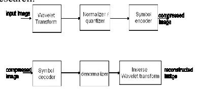
Figure 4: Image Compression Using Wavelets
4. ERROR METRICS
Two of the error metrics [1] used to compare the various image compression techniques are the Mean Square Error (MSE) and the Peak Signal to Noise Ratio (PSNR) to achieve desirable compression ratios. The MSE is the cumulative squared error between the compressed and the original image, whereas PSNR is a measure of the peak error. The mathematical formulae for the two are:
where I(x,y) is the original image, I'(x,y) is the approximated version (which is actually the decompressed image) and M,N are the dimensions of the images. A lower value for MSE means lesser error, and as seen from the inverse relation between the MSE and PSNR, this translates to a high value of PSNR. Logically, a higher value of PSNR is good because it means that the ratio of Signal to Noise is higher. Here, the 'signal' is the original image, and the 'noise' is the error in reconstruction. So, if you find a compression scheme having a lower MSE (and a high PSNR), you can recognize that it is a better one.
4.1 DATA COMPRESSION
TRANSFORMATION
Data compression ratio [5], also
known as compression power, is used to
quantify
the
reduction
in
video, the compression ratio is defined in
terms of uncompressed and compressed data
rates instead of data sizes.
When the uncompressed data rate is
known, the compression ratio can be
inferred from the compressed data rate.
4.2 MEAN SQUARE ERROR (MSE)
Mean square error [1] is a criterion for an estimator: the choice is the one that minimizes the sum of squared errors due to bias and due to variance. The average of the square of the difference between the desired response and the actual system output. As a loss function, MSE is called squared error loss. MSE measures the average of the square of the "error. The MSE is the second moment (about the origin) of the error, and thus incorporates both the variance of the estimator and its bias. For an unbiased estimator, the MSE is the variance. In an analogy to standard deviation, taking the square root of MSE yields the root mean squared error or RMSE. Which has the same units as the quantity being estimated. For an unbiased estimator, the RMSE is the square root of the variance, known as the standard error.
Where m x n is the image size and I(i, j) is the input image and K(i, j) is the retrieved image.
4.3 PEAK SIGNAL-TO-NOISE RATIO (PSNR)
PSNR [4] is the ratio of maximum power of the signal and the power of unnecessary distorting noise. Here the signal is the original image and the noise is the error in reconstruction. For a better compression the PSNR must be high. Because many signals have a very wide dynamic range, PSNR [1] is usually expressed in terms of the logarithmic decibel scale. The PSNR is most commonly used as a measure of quality of reconstruction in image compression etc. It is most easily defined via the mean squared error (MSE) which for two m×n monochrome images I and K where one of the images is considered noisy.
Here, MAXi is the maximum possible pixel value of the image. When the pixels are represented using 8 bits per sample, this is 255. Typical values for the PSNR in Lossy image and video compression are between 30 and 50 dB, where higher is better. PSNR is computed by measuring the pixel difference between the original image and compressed image. Values for PSNR range between infinity for identical images, to 0 for images that have no commonality. PSNR decreases as the compression ratio increases for an image.
4. CONCLUSION
In this survey paper, we have discussed various up-to-date image compressions for neural network and wavelet transformation according to their applications and design. Theoretically, all the existing image compression techniques can be possibly implemented by neural network structures and wavelet transformation. Indirect neural applications are developed to assist with traditional techniques and provide a very good potential for further improvement on conventional image coding and compression techniques. At first the fundamental theory of artificial neural network (ANN) and wavelet theory with wavelet transformation have reviewed.
5. REFERENCES