Connectivity problems on heterogeneous graphs

RESEARCH

Connectivity problems on heterogeneous

graphs

Jimmy Wu

_{, Alex Khodaverdian}

_{, Benjamin Weitz}

_{and Nir Yosef}

Abstract

Background: Network connectivity problems are abundant in computational biology research, where graphs are used to represent a range of phenomena: from physical interactions between molecules to more abstract relation-ships such as gene co-expression. One common challenge in studying biological networks is the need to extract meaningful, small subgraphs out of large databases of potential interactions. A useful abstraction for this task turned out to be the Steiner Network problems: given a reference “database” graph, find a parsimonious subgraph that satisfies a given set of connectivity demands. While this formulation proved useful in a number of instances, the next challenge is to account for the fact that the reference graph may not be static. This can happen for instance, when studying protein measurements in single cells or at different time points, whereby different subsets of conditions can have different protein milieu.

Results and discussion: We introduce the condition Steiner Network problem in which we concomitantly consider a set of distinct biological conditions. Each condition is associated with a set of connectivity demands, as well as a set of edges that are assumed to be present in that condition. The goal of this problem is to find a minimal subgraph that satisfies all the demands through paths that are present in the respective condition. We show that introducing mul-tiple conditions as an additional factor makes this problem much harder to approximate. Specifically, we prove that for C conditions, this new problem is NP-hard to approximate to a factor of C−ǫ , for every C ≥2 and ǫ >0 , and that

this bound is tight. Moving beyond the worst case, we explore a special set of instances where the reference graph grows monotonically between conditions, and show that this problem admits substantially improved approximation algorithms. We also developed an integer linear programming solver for the general problem and demonstrate its ability to reach optimality with instances from the human protein interaction network.

Conclusion: Our results demonstrate that in contrast to most connectivity problems studied in computational biol-ogy, accounting for multiplicity of biological conditions adds considerable complexity, which we propose to address with a new solver. Importantly, our results extend to several network connectivity problems that are commonly used in computational biology, such as Prize-Collecting Steiner Tree, and provide insight into the theoretical guarantees for their applications in a multiple condition setting.

Keywords: Steiner Network, NP hard, Approximation algorithm, Protein–protein interaction

© The Author(s) 2019. This article is distributed under the terms of the Creative Commons Attribution 4.0 International License (http://creat iveco mmons .org/licen ses/by/4.0/), which permits unrestricted use, distribution, and reproduction in any medium, provided you give appropriate credit to the original author(s) and the source, provide a link to the Creative Commons license, and indicate if changes were made. The Creative Commons Public Domain Dedication waiver (http://creat iveco mmons .org/ publi cdoma in/zero/1.0/) applies to the data made available in this article, unless otherwise stated.

Open Access

*Correspondence: niryosef@eecs.berkeley.edu

2 _{Department of Electrical Engineering and Computer Science, UC} Berkeley, Berkeley, CA, USA

Background

In molecular biology applications, networks are routinely defined over a wide range of basic entities such as pro-teins, genes, metabolites, or drugs, which serve as nodes. The edges in these networks can have different meanings, depending on the particular context. For instance, in pro-tein–protein interaction (PPI) networks, edges represent physical contact between proteins, either within stable multi-subunit complexes or through transient causal interactions (i.e., an edge (x, y) means that protein x can cause a change to the molecular structure of protein y and thereby alter its activity). The body of knowledge encapsulated within the human PPI network (tens of thousands of nodes and hundreds of thousands of edges in current databases, curated from thousands of studies [1]) is routinely used by computational biologists to gen-erate hypotheses of how various signals are transduced in eukaryotic cells [2–6]. The basic premise is that a process that starts with a change to the activity of protein u and ends with the activity of protein v must be propagated through a chain of interactions between u and v. The nat-ural extension regards a process with a certain collection of protein pairs {(u₁,v₁),. . .,(u_k,v_k)} , where we are look-ing for a chain of interactions between each ui and vi [7]. In another set of applications, the notion of directionality is not directly assumed and instead, one is looking for a parsimonious subgraph that connects together a set S of proteins that are postulated to be active [8, 9].

In most applications, the identity of the so called termi-nal nodes (i.e., (u_i,v_i) pairs or the set S) is assumed to be

known (or inferred from experimental data such as ChIP-seq [5, 8, 9]), while the identity of the intermediate nodes and interactions is unknown. The goal therefore becomes to complete the gap and find a probable subgraph of the PPI network that simultaneously satisfies all the connec-tivity demands, thereby explaining the overall biologi-cal activity. Since the edges in the PPI network can be assigned a probability value (reflecting the credibility of their experimental evidence), by taking the negative log of these values as edge weights, the task becomes mini-mizing the total edge weight, leading to an instance of the Steiner Network problem. We have previously used this approach to study the propagation of a stabilizing signal in pro-inflammatory T cells, leading to the identification of a new molecular pathway (represented by a sub-graph of the PPI network) that is critical for mounting an auto-immune response, as validated experimentally by pertur-bation assays and disease models in mice [5]. Tuncbag et al. [9] have utilized the undirected approach using the Prize-Collecting Steiner Tree model, where the input is a network G along with a penalty function, p(v) for each protein (node) in the network (based on their impor-tance; e.g., fold-change across conditions). The goal in

this case is to find a probable subtree which contains the majority of the high cost proteins in G, while accounting for penalties paid by both edge usage and missing pro-teins, in order to capture the biological activity repre-sented in such a network [8, 9].

While these studies contributed to our understanding of signal transduction pathways in living cells, they do not account for a critical aspect of the underlying biologi-cal complexity. In reality, proteins (nodes) can become activated or inactivated at different conditions, thereby giving rise to a different set of potential PPIs that might take place [10]. Here, the term condition can refer to dif-ferent points in time [11], difdif-ferent treatments [12], or, more recently, different cells [13]. Indeed, advances in experimental proteomics provide a way to estimate these changes at high throughput, e.g., measuring phosphoryl-ation levels or overall protein abundance, proteome-wide for a limited number of samples [12]. A complementary line work provides a way to evaluate the abundance of smaller numbers of proteins (typically dozens of them) in hundreds of thousands of single cells [13].

The next challenge is therefore to study connectivity problems that take into account not only the endpoints of each demand, but also the condition in which these demands should be satisfied. This added complication was tackled by Mazza et  al. [14], who introduced the “Minimum k-Labeling (MKL)” problem. In this setting, each connectivity demand comes with a label, which rep-resents a certain experimental condition or time point. The task is to label edges in the PPI network so as to sat-isfy each demand using its respective label, while mini-mizing the number of edges in the resulting sub-graph and the number of labels used to annotate these edges. While MKL was an important first step, namely intro-ducing the notion of different demands for each condi-tion, the more difficult challenge still remains that of considering variability in the reference graph, namely dif-ferent sets of proteins that may be active and available for use in each condition. To this effect, we note the exist-ence of multi-layer networks in the data-mining space. In this context, studies have focused on networks which have edges that span across specified dimensions, or con-ditions [15, 16]. However, we could not find studies that tackle the problem of parsimonious connectivity in this domain.

Summary of main contributions

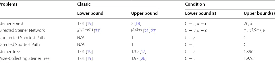
over a sequence of graphs Gc defined over each condition, where vertices remain the same, but edges are allowed to change across conditions (notably, our results also hold when Gc is defined with changing vertices rather than edges). Furthermore, demands are in the form of “con-nect node u to node v through a path of nodes that are present in condition c”. The goal is to find a minimum-weight subgraph of G that satisfies all the demands (Fig. 1).

We first show that it is NP-hard to find a solution that achieves a nontrivial approximation factor (by the “triv-ial” approximation, we mean the one obtained by solv-ing the problem independently for each condition). This result extends to several types of connectivity problems and provides a theoretical lower bounds to the best-pos-sible approximation guarantee that can be achieved in a multiple condition setting (Table 1). For instance, we can conclude that concomitantly solving the shortest path problem for a set of conditions is hard to approximate,

and that the trivial solution (i.e., solving the problem to optimality in each condition) is, theoretically, the best that one can do. Another example, commonly used in PPI analysis, is the Prize-Collecting Steiner Tree problem [8, 9]. Here, our results indicate that given a fixed input for this problem (i.e., a penalty function p(v) for each ver-tex), it is NP-hard to solve it concomitantly in C condi-tions, such that the weight of the obtained solution is less than C times that of the optimal solution. Interestingly, a theoretical guarantee of C·(2− 2

|V|)

1 _{can be obtained} by solving the problem independently for each time point

While these results provide a somewhat pessimis-tic view, they rely on the assumption that the network frames Gc are arbitrary. In the last part of this paper, we show that for the specific case where the conditions can be ordered such that each condition is a subset of the Fig. 1 Examples of well studied network problems (a), and their corresponding extension with multiple conditions (b). The problems shown are: Undirected Steiner Tree, Directed Steiner Network, and Shortest Path, respectively. Yellow nodes and red edges correspond to nodes and edges used in the optimal solutions for the corresponding instances

Table 1 Approximation bounds for the various Steiner Network Problems in their classic setting and condition setting

For the classic problems, we have indicated the papers in which the bounds are shown. For the condition problems, all the lower bounds are developed in the present work; all the upper bounds are the naive bounds obtained from the “union of shortest paths” heuristic, or from applying the best known approximation algorithm for the appropriate classic Steiner problem to each condition, then taking the union of those solutions

Problems Classic Condition

Lower bound Upper bound Lower bound(s) Upper bound(s)

Steiner Forest 1.01 [19] 2 [18] C−ǫ,k−ǫ 2C, k

Directed Steiner Network k1/4−o(1) _{[27] k}1/2+ǫ

[21, 22] C−ǫ,k−ǫ C·k1/2+ǫ_,k

Undirected Shortest Path N/A 1 C−ǫ C

Directed Shortest Path N/A 1 C−ǫ C

Steiner Tree 1.01 [19] 1.39 [17] C−ǫ 1.39C

Prize-Collecting Steiner Tree 1.01 [19] 1.97 [26] C−ǫ 1.97C

next (namely, Gc⊆Gc′ for c≤c′ ) then the CSN problem

can be reduced to a standard connectivity problem with a single condition, leading to substantially better theo-retical guarantees. Finally, we develop an integer linear program for the general CSN problem, and show that provided with real-world input (namely, the human PPI) it is capable of reaching an optimal solution in a reason-able amount of time.

Introduction to Steiner problems

The Steiner Tree problem, along with its many variants and generalizations, form a core family of NP-hard com-binatorial optimization problems. Traditionally, the input to one of these problems is a single (usually weighted) graph, along with requirements about which nodes need to be connected in some way; the goal is to pick a minimum-weight subgraph satisfying the connectivity demands.

In this paper, we offer a multi-condition perspective; in our setting, multiple graphs over the same vertex set (which one can think of as an initial graph changing over a set of discrete conditions), are all given as input, and the goal is to pick a subgraph satisfying condition-sensi-tive connectivity requirements. Our study of this prob-lem draws motivation and techniques from several lines of research, which we briefly summarize.

Classic Steiner problems

A basic problem in graph theory is finding the short-est path between two nodes; this problem is efficiently solved using, for example, Dijkstra’s algorithm.

A natural extension of this is the Steiner Tree prob-lem: given a weighted undirected graph G=(V,E) and

a set of terminals T ⊆V , find a minimum-weight subtree

that connects all the nodes in T. A further generalization is Steiner Forest: given G=(V,E) and a set of demand

pairs D⊆V×V , find a subgraph that connects each

pair in D. Currently the best known approximation algo-rithms give a ratio of 1.39 for Steiner Tree [17] and 2 for Steiner Forest [18]. These problems are known to be NP-hard to approximate to within some small constant [19].

For directed graphs, we have the Directed Steiner Network (DSN) problem, in which we are given a weighted directed graph G=(V,E) and k demands (a1,b1),. . .,(a_k,b_k)∈V×V , and must find a mini-mum-weight sub-graph in which each ai has a path to bi . When k is fixed, DSN admits a polynomial-time exact algorithm [20]. For general k, the best known approxima-tion algorithms have ratio O(k1/2+ǫ) for any fixed ǫ >0 [21, 22]. On the complexity side, Dodis and Khanna [23] ruled out a polynomial-time O(2log

1−ǫ_n

)-approximation for this problem unless NP has quasipolynomial-time

algorithms.2 _{An important special case of DSN is} Directed Steiner Tree, in which all demands have the form (r,b_i) for some root node r. This problem has an

O(kǫ)-approximation scheme [24] and a lower bound of

� (log2−ǫn) [25].

Finally, a Steiner variant that has found extensive use in computational biology is the Prize-Collecting Steiner Tree problem, in which the input contains a weighted undirected graph G=(V,E) and penalty function

p:V →_R≥0 ; the goal is to find a subtree which

simul-taneously minimizes the weights of the edges in the tree and the penalties paid for nodes not included within the tree, i.e. cost(T):=_e

∈Tw(e)+

v∈/Tp(v) . For this

problem, an approximation algorithm with ratio 1.967 is known [26].

Condition Steiner problems

In this paper, we generalize the Shortest Path, Steiner Tree, Steiner Forest, Directed Steiner Network, and Prize-Collecting Steiner Tree problems to the multi-condition setting. In this setting, we have a set of con-ditions [C] := {1,. . .,C} , and are given a graph for each condition.

Our main object of study is the natural generalization of Steiner Forest (in the undirected case) and Directed Steiner Network (in the directed case), which we call Condition Steiner Network:

Definition 1 (Condition Steiner Network (CSN)) We are given the following inputs:

1. A sequence of undirected graphs

G1=(V,E₁),G₂=(V,E₂),. . .,G_C =(V,E_C) , one for each conditionc∈ [C] . Each edge e in the

under-lying edge set E :=_cEc has a weight w(e)≥0.

2. A set of k connectivity demandsD⊆V ×V × [C] . We assume that for every c∈C there exists at least

one demand and therefore that k≥ |C|.

We call G=(V,E) the underlying graph. We say a

sub-graph H ⊆Gsatisfies demand (a,b,c)∈D if H contains an a-b path P along which all edges exist in Gc . The goal is to output a minimum-weight subgraph H⊆G that satis-fies every demand in D.

Definition 2 (Directed Condition Steiner Network (DCSN)) This is the same as CSN except that all the edges

are directed, and a demand (a, b, c) must be satisfied by a directed path from a to b in Gc.

We can also define the analogous generalizations of Shortest Path, (undirected) Steiner Tree, and Prize-Col-lecting Steiner Tree. We give hardness results and algo-rithms for these problems by demonstrating reductions to and from CSN and DCSN.

Definition 3 (Condition Shortest Path (CSP), Directed Condition Shortest Path (DCSP)) These are the special cases of CSN and DCSN in which the demands are pre-cisely (a,b, 1),. . .,(a,b,C) where a,b∈V are common source and target nodes.

Definition 4 (Condition Steiner Tree (CST)) We are given a sequence of undirected graphs G1=(V,E₁),. . .,G_C =(V,E_C) , a weight w(e)≥0 on each e∈E , and sets of terminal nodes X₁,. . .,X_C ⊆V . We say a subgraph H ⊆(V,

cEc)satisfies the terminal set Xc if the nodes in Xc are mutually reachable using

edges in H that exist at condition c. The goal is to find a minimum-weight subgraph H that satisfies Xc for every c∈ [C].

Definition 5 (Condition Prize-Collecting Steiner Tree (CPCST)) We are given a sequence of undirected graph G1=(V,E₁),. . .,G_C =(V,E_C), a weight w(e)≥0 on each e∈E, and a penalty p(v,c)≥0 for each

v∈V,c∈ [C] . The goal is to find a subtree T that

mini-mizes

e∈Tw(e)+

v∈/T,c∈[C]p(v,c).

Finally, in molecular biology applications, it is often the case that all the demands originate from a common root node. To capture this, we define the following special case of DCSN:

Definition 6 (Single-Source DCSN) This is the spe-cial case of DCSN in which the demands are precisely

(a,b₁,c₁),(a,b₂,c₂),. . .,(a,b_k,c_k) , for some root a∈V . We can assume that c1≤c2≤ · · · ≤ck.

It is also natural to consider variants of these problems in which nodes (rather than edges) vary across the condi-tions, or in which both nodes and edges vary. In Problem variants, we show that all three variants are in fact equiv-alent; thus we focus on the edge-based formulations.

Our results

In this work, we perform a systematic study of the con-dition Steiner problems defined above, from the stand-point of approximation algorithms—that is, algorithms that return subgraphs whose total weights are not much

greater than that of the optimal subgraph—as well as integer linear programming (ILP). Since all of the condi-tion Steiner problems listed in the previous seccondi-tion turn out to be NP-hard (and in fact all of them except Shortest Path are hard even in the classic single-condition setting) we cannot hope for algorithms that find optimal solu-tions and run in polynomial time.

First, in Hardness of condition Steiner problems, we show a series of strong negative results, starting with (directed and undirected) Condition Steiner Network:

Theorem 1 (Main Theorem) CSN and DCSN are NP-hard to approximate to a factor of C−ǫas well as k−ǫ for every fixed k≥2 and every constant ǫ >0 . For DCSN, this holds even when the underlying graph is acyclic.

Thus the best approximation ratio one can hope for

is C or k; the latter upper bound is easily achieved by

the trivial “union of shortest paths” algorithm: for each demand (a, b, c), compute the shortest a-b path at condi-tion c; then take the union of these k paths. This contrasts with the classic Steiner Network problems, which have nontrivial approximation algorithms and efficient fixed-parameter algorithms.

Next, we show similar hardness results for the other three condition Steiner problems. This is achieved by a series of simple reductions from CSN and DCSN.

Theorem  2 Condition Shortest Path, Directed Condi-tion Shortest Path, CondiCondi-tion Steiner Tree, and CondiCondi-tion Prize-Collecting Steiner Tree are all NP-hard to approxi-mate to a factor of C−ǫ for every fixed C≥2 and ǫ >0.

Note that each of these condition Steiner problems can be naively approximated by applying the best known algorithm for the classic version of that problem in each graph in the input, then taking the union of all those sub-graphs. If the corresponding classic Steiner problem can be approximated to a factor of α , then this process gives an α·C-approximation for the condition version. Thus using known constant-factor approximation algorithms, each of the condition problems in Theorem 2 has an O(C)-approximation algorithm. Our result shows that in the worst case, one cannot do much better.

While these results provide a somewhat pessimistic view, the proofs rely on the assumption that the edge sets in the input networks (that is, E1,. . .,EC ) do not necessarily bear any relationship to one another. In Monotonic special cases, we move beyond this worst-case assumption by studying a broad class of special cases in which the conditions are monotonic: if an edge e exists in some graph Gc , then it exists in all the

the input is a subgraph of the next. For these problems, we prove the following two theorems:

Theorem  3 Monotonic CSN has a

polynomial-time O(logk)-approximation algorithm. It has

no � (log logn)-approximation algorithm unless

NP⊆DTIME(nlog log logn).

In the directed case, for monotonic DCSN with a sin-gle source (that is, every demand is of the form (r, b, c) for a common root node r), we show the following:

Theorem 4 Monotonic Single-Source DCSN has a

pol-ynomial-time O(kǫ)-approximation algorithm for every

ǫ >0 . It has no � (log2−ǫn)-approximation algorithm

unless NP⊆ZPTIME(npolylog(n)).

These bounds are proved via approximation-preserv-ing reductions to and from classic Steiner problems, namely Priority Steiner Tree and Directed Steiner Tree. Conceptually, this demonstrates that imposing the monotonicity requirement makes the condition Steiner problems much closer to their classic counterparts, allowing us to obtain algorithms with substantially bet-ter approximation guarantees.

Finally in application to protein–protein interac-tion networks, we show how to model various condi-tion Steiner problems as integer linear programs (ILPs). In experiments on real-world inputs derived from the human PPI network, we find that these ILPs are capable of reaching optimal solutions in a reasonable amount of time.

Table 1 summarizes our results, emphasizing how the known upper and lower bounds change when going from the classic Steiner setting to the condition Steiner setting.

Preliminaries

Note that the formulations of CSN and DCSN in the introduction involved a fixed vertex set; only the edges change over the conditions. It is also natural to formu-late the Condition Steiner Network problem with nodes changing over condition, or both nodes and edges. However by the following proposition, it is no loss of generality to discuss only the edge-condition variant.

Proposition 1 The edge, node, and node-and-edge var-iants of CSN are mutually polynomial-time reducible via strict reductions (i.e. preserving the approximation ratio exactly). Similarly all three variants of DCSN are mutu-ally strictly reducible.

We defer the precise definitions of the other two vari-ants, as well as the proof of this proposition, to Problem variants.

In this edge-condition setting, it makes sense to define certain set operations on graphs, which will be of use in our proofs. To that end, let G1=(V,E₁) and G2=(V,E₂) be two graphs on the same vertex set. Their union, G1∪G2 , is defined as (V,E₁∪E2) . Their intersec-tion, G1∩G2 , is defined as (V,E₁∩E2) . Subset relations are defined analogously; for example, if E1⊆E2 , then we say that G1⊆G2.

Next we state the Label Cover problem, which is the starting point of one of our reductions to CSN.

Definition 7 (Label Cover (LC)) An instance of this problem consists of a bipartite graph G=(U,V,E) and a set of possible labels . The input also includes, for each edge (u,v)∈E , projection functions π

(u,v)

u :�→C

and π (u,v)

v :�→C , where C is a common set of colors;

�= {π_ve:e∈E,v∈e} is the set of all such func-tions. A labeling of G is a function φ:U∪V →� assigning each node a label. We say a labeling φ satis-fies an edge (u,v)∈E , or (u, v) is consistent under φ , if

π

(u,v)

u (φ (u))=π

(u,v)

v (φ (v)) . The task is to find a labeling

that satisfies as many edges as possible.

This problem was first defined in [28]. It has the follow-ing gap hardness, as shown by Arora et al. [29] and Raz [30].

Theorem 5 For every ǫ >0 , there is a constant || such that the following promise problem is NP-hard: Given a Label Cover instance (G,�,�) , distinguish between the following cases:

• (YES instance) There exists a total labeling ofG; i.e. a labeling that satisfies every edge.

• (NO instance) There does not exist a labeling ofGthat satisfies more thanǫ|E|edges.

Hardness of condition Steiner problems Overview of the reduction

Here we outline our strategy for reducing Label Cover to the condition Steiner problems. First, we reduce to the CSN problem restricted to having only C=2 condi-tions and k=2 demands; we call this problem 2-CSN. The directed problem  2-DCSN is defined analogously. Later, we obtain similar hardness for CSN with more conditions or demands by using the same ideas, but reducing from k-Partite Hypergraph Label Cover.

Consider the nodes u1,. . .,u|U_| on the “left” side of the LC instance. We build, for each ui , a gadget (which is a small sub-graph in the Steiner instance) consisting of multiple parallel directed paths from a source to a sink—one path for each possible label for ui . We then chain together these gadgets, so that the sink of u1 ’s

gadget is the source of u2 ’s gadget, and so forth. Finally we create a connectivity demand from the source of u1 ’s gadget to the sink of u|U| ’s gadget, so that a solu-tion to the Steiner instance must have a path from u1 ’s

gadget, through all the other gadgets, and finally ending at u|U| ’s gadget. This path, depending on which of the parallel paths it takes through each gadget, induces a labeling of the left side of the Label Cover instance. We build an analogous chain of gadgets for the nodes on the right side of the Label Cover instance.

The last piece of the construction is to ensure that the Steiner instance has a low-cost solution if and only if the Label Cover instance has a consistent labeling. This is accomplished by setting all the ui gadgets to exist only at condition 1 (i.e. in frame G1 ), setting the

vj gadgets to exist only in G2 , and then merging cer-tain edges from the ui-gadgets with edges from the vj -gadgets, replacing them with a single, shared edge that exists in both frames. Intuitively, the edges we merge are from paths that correspond to labels that satisfy the Label Cover edge constraints. The result is that a YES instance of Label Cover (i.e. one with a total labeling) will enable a high degree of overlap between paths in the Steiner instance, so that there is a very low-cost solution. On the other hand, a NO instance of LC will

not result in much overlap between the Steiner gadgets, so every solution will be costly.

Let us define some of the building blocks of the reduction we just sketched:

• A simple strand is a directed path of the form

b1→c₁→c₂→b₂.

• In a simple strand, we say that (c₁,c₂) is the contact edge. Contact edges have weight 1; all other edges in our construction have zero weight.

• A bundle is a graph gadget consisting of a source node b1 , sink node b2 , and parallel, disjoint strands from b1 to b2.

• A chain of bundles is a sequence of bundles, with the sink of one bundle serving as the source of another. • More generally, a strand can be made more

compli-cated, by replacing a contact edge with another bundle (or even a chain of them). In this way, bundles can be nested, as shown in Fig. 2.

• We can merge two or more simple strands from dif-ferent bundles by setting their contact edges to be the same edge, and making that edge existent at the union of all conditions when the original edges existed (Fig. 2).

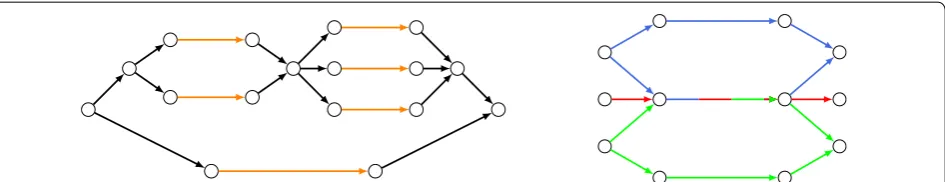
Before formally giving the reduction, we illustrate a simple example of its construction.

Our reduction outputs this corresponding 2-CSN instance:

G1 comprises the set of blue edges; G2 is green. The

demands are (uS

1,uS2, 1) and (vS1,v2S, 2) . For the Label Cover node u, G1 (the blue sub-graph) consists of two strands,

one for each possible label. For the Label Cover node v, G2 (green sub-graph) consists of one simple strand for the label ‘1’, and a bundle for label ‘2’, which branches out into two simple strands, one for each agreeing labeling of u. Finally, strands (more precisely, their contact edges) whose labels map to the same color are merged.

The input is a YES instance of Label Cover whose opti-mal labelings (u gets either label 1 or 2, v gets label 2) correspond to 2-CSN solutions of cost 1 (both G1 and

G2 contain the (u,  1, v,  2)-path, and both contain the (u, 2, v, 2)-path). If this were a NO instance and edge e could not be satisfied, then the resulting 2-CSN sub-graphs G1 and G2 would have no overlap.

Inapproximability for two demands

We now formalize the reduction in the case of two condi-tions and two demands; later, we extend this to general C and k.

Theorem  6 2-CSN and 2-DCSN are NP-hard to approximate to within a factor of 2−ǫ for every constant ǫ >0 . For 2-DCSN, this holds even when the underlying graph is acyclic.

Proof Fix any desired ǫ >0 . We describe a reduction from Label Cover (LC) with any parameter ε < ǫ (that is, in the case of a NO instance, no labeling satisfies more than an ε-fraction of edges) to 2-DCSN with an acyclic graph. Given the LC instance (G=(U,V,E),�,�) , construct a 2-DCSN instance ( G=(G₁,G₂) , along with two connec-tivity demands) as follows. Create nodes uS₁,. . .,uS

|U|+1

and v₁S,. . .,vS

|V|+1 . Let there be a bundle from each uSi to uS_i+1 ; we call this the ui-bundle, since a choice of path from uS_i to uS_i+1 in G will indicate a labeling of ui in G.

The ui-bundle has a strand for each possible label ℓ∈� . Each of these ℓ-strands consists of a chain of bun-dles—one for each edge (ui,v)∈E . Finally, each such

(ui,ℓ,v)-bundle has a simple strand for each label r∈ such that π_u(ui,v)

i (ℓ)=π

(u_i,v)

v (r) ; call this the (ui,ℓ,v,r)

-path. In other words, there is ultimately a simple strand for each possible labeling of ui ’s neighbor v such that the two nodes are in agreement under their mutual edge con-straint. If there are no such consistent labels r, then the (ui,ℓ,v)-bundle consists of just one simple strand, which is not associated with any r. Note that every minimal uS₁→uS|U|+1 path (that is, one that proceeds from one

bundle to the next) has total weight exactly |E|.

Similarly, create a vj-bundle from each vS_j to vS_j+1 , whose

r-strands (for r∈ ) are each a chain of bundles, one for

each (u,v_j)∈E . Each (u,r,v_j)-bundle has a (u,ℓ,vj,r) -path for each agreeing labeling ℓ of the neighbor u, or a simple strand if there are no such labelings.

Set all the edges in the ui-bundles to exist in G1 only.

Similarly the vj-bundles exist solely in G2 . Now, for each

(u,ℓ,v,r)-path in G₁ , merge it with the (u,ℓ,v,r)-path in

G2 , if it exists. The demands are

D=

uS₁,uS_|U|+1, 1,v₁S,vS_|V|+1, 2.

We now analyze the reduction. The main idea is that any uS_i →uS_i+1 path induces a labeling of ui ; thus the

demand uS₁,uS|U|+1, 1

ensures that any 2-DCSN solution indicates a labeling of all of U. Similarly, v₁S,vS_|V|+1, 2

forces an induced labeling of V. In the case of a YES instance of Label Cover, these two connectivity demands can be satisfied by taking two paths with a large amount of overlap, resulting in a low-cost 2-DCSN solution. In contrast when we start with a NO instance of Label Cover, any two paths we can choose to satisfy the 2-DCSN demands will be almost completely disjoint, resulting in a costly solution. We now fill in the details.

Suppose the Label Cover instance is a YES instance, so that there exists a labeling ℓ∗u to each u∈U , and rv to each ∗ _v∈V , such that for all edges _(u,v)∈E ,

π (_u,v) u (ℓ∗

u)=π (_u,v) v (r∗

v) . The following is an optimal solu-tion H∗ _{to the constructed 2-DCSN instance:}

• To satisfy the demand at condition 1, for each

u-bundle, take a path through the ℓ∗

u-strand. In

par-ticular for each (u,ℓ∗

u,v)-bundle in that strand,

trav-erse the (u,ℓ∗

• To satisfy the demand at condition 2, for each

v-bundle, take a path through the r_{v-strand. In par-}∗

ticular for each (u,r∗

v,v)-bundle in that strand,

trav-erse the (u,ℓ∗

u,v,rv∗)-path.

In tallying the total edge cost, H∗_∩G1 (i.e. the sub-graph at condition 1) incurs a cost of |E|, since one con-tact edge in G is encountered for each edge in G. H∗_∩G2

accounts for no additional cost, since all contact edges correspond to a label which agrees with some neighbor’s label, and hence were merged with the agreeing contact edge in H∗_∩G1 . Clearly a solution of cost |E| is the best

possible, since every uS₁→uS_|U|+1 path in G1 (and every vS₁→v_|VS _|+1 path in G2 ) contains at least |E| contact

edges.

Conversely suppose we started with a NO instance of Label Cover, so that for any labeling ℓ∗u to u and r_v∗ to v, for at least (1−ε)|E| of the edges (u,v)∈E , we have π

(u,v)

u (ℓ∗_u)�=π (u,v)

v (r_v∗). By definition, any solution to the constructed 2-DCSN instance contains a simple uS₁→uS_|U|+1 path P1∈G1 and a simple v1S→v|VS |+1 path

P2∈G2 . P1 alone incurs a cost of exactly |E|, since one contact edge in G is traversed for each edge in G. However, P1 and P2 share at most ε|E| contact edges (otherwise, by the merging process, this implies that more than ε|E| edges could be consistently labeled, which is a contradiction). Thus the solution has a total cost of at least (2−ε)|E|.

It is thus NP-hard to distinguish between an instance with a solution of cost |E|, and an instance for which every solution has cost at least (2−ε)|E| . Thus a

pol-ynomial-time algorithm for 2-DCSN with approxima-tion ratio 2−ǫ can be used to decide Label Cover (with parameter ε ) by running it on the output of the aforemen-tioned reduction. If the estimated objective value is at most (2−ε)|E| (and thus strictly less than (2−ǫ )|E| )

out-put YES; otherwise outout-put NO. In other words, 2-DCSN is NP-hard to approximate to within a factor of 2−ǫ.

To complete the proof, observe that the underlying directed graph we constructed is acyclic, as every edge points “to the right” as in Example 1. Hence 2-DCSN is NP-hard to approximate to within a factor of 2−ǫ for every ǫ >0 , even on acyclic graphs. Finally, note that the same analysis holds for 2-CSN, by simply making every edge undirected; however in this case the graph is clearly

not acyclic.

Inapproximability for general C and k

Theorem 1 (Main Theorem) CSN and DCSN are NP-hard to approximate to a factor of C−ǫas well as k−ǫ for every fixed k≥2 and every constant ǫ >0 . For DCSN, this holds even when the underlying graph is acyclic.

Proof We perform a reduction from k-Partite Hypergraph Label Cover, a generalization of Label Cover to hyper-graphs, to CSN, or DCSN with an acyclic graph. Using the same ideas as in the C=k=2 case, we design k demands composed of parallel paths corresponding to labelings, and merge edges so that a good global labeling corresponds to a large overlap between those paths. The full proof is left to

Proof of inapproximability for general C and k.

Note that a k-approximation algorithm is to simply choose H=_ciP˜ci , where _P˜

ci is the shortest aci→bci path in Gci for demands D= {(a,b,ci):ci∈ [C]} . Thus by Theorem 1, essentially no better approximation is pos-sible in terms of k alone. In contrast, most classic Steiner problems have good approximation algorithms [21, 22, 24, 25], or are even exactly solvable for constant k [20].

Inapproximability for Steiner variants

We take advantage of our previous hardness of approxi-mation results in Theorem 1 and show, via a series of reductions, that CSP, CSN, and CPCST are also hard to approximate.

Theorem  2 Condition Shortest Path, Directed Condi-tion Shortest Path, CondiCondi-tion Steiner Tree, and CondiCondi-tion Prize-Collecting Steiner Tree are all NP-hard to approxi-mate to a factor of C−ǫ for every fixed C≥2 and ǫ >0.

Proof We first reduce from CSN to CSP (and DCSN to DCSP). Suppose we are given an instance of CSN with graph sequence G=(G₁,. . .,G_C) ,

underlying graph G=(V,E), and demands

D= {(a_i,b_i,c_i):i∈ [k]}. We build a new instance

G′

=(G′

1,. . .,Gk′),G ′

=(V′,E′),D′ as follows.

Initialize G′ _{to G. Add to G}′ _{the new nodes a and b, which}

exist at all conditions G_{i . For all} ′ _{e∈E and i∈ [k] , if e∈G}

ci ,

then let e exist in G_{i as well. For each} ′ _(a

i,bi,ci)∈D,

1. Create new nodes xi , yi . Create zero-weight edges

(a,x_i) , (x_i,a_i) , (bi,y_i) , and (yi,b).

2. Let (a,x_i) , (x_i,a_i) , (bi,y_i) , and (yi,b) exist only in frame G′

i.

Lastly, the demands are D′

= {(a,b,i):i∈ [k]}.

Given a solution H′

⊆G′ containing an a→b path at every condition i∈ [k] , we can simply exclude nodes a,

b, {x_i} , and {y_i} to obtain a solution H⊆G to the origi-nal instance, which contains an ai→bi path in Gci for all i∈ [k] , and has the same cost. The converse is also true

Observe that essentially the same procedure shows that DCSN reduces to DCSP; simply ensure that the edges added by the reduction are directed rather than undirected.

Next, we reduce CSP to CST. Suppose we are given an instance of CSP with graph sequence G=(G₁,. . .,G_C), underlying graph

G=(V,E), and demands D= {(a,b,i):i∈ [C]} . We build a new instance of CST as follows:

G′_=(G′

1,. . .,GC′),G′=(V′,E′),X =(X1,. . .,X_C) . Set

G′ _{to G , and G}′ _{to G. Take the set of terminals in each} con-dition to be Xi= {a,b} . We note that a solution H′⊆G′

to the CST instance is trivially a solution the CSP instance with the same cost, and vice-versa.

Finally, we reduce CST to CPCST. We do this by making an appropriate assignment of the penalties p(v, c). Sup-pose we are given an instance of CST with graph sequence

G=(G₁,. . .,G_C) , underlying graph G=(V,E) , and

ter-minal sets X =(X₁,. . .,X_C) . We build a new instance

of CPCST,

G′_=(G′

1,. . .,GC′ ),G′=(V′,E′),p(v,c)

. In particular, set G′ _{to G , and G}′ _{to G. Set p(v, c) as follows:}

Consider any solution H ⊆G to the original CST instance. Since H spans the terminals X1,. . .,X_c (thus avoiding any infinite penalties), and since the non-termi-nal vertices have zero cost, the overall cost of H remains the same cost in the constructed CPCST instance. Con-versely, suppose we are given a solution H′_⊆G′ to the constructed CPCST instance. If the cost of H′ is _∞ , then

H′ does not span all the _X

c ’s simultaneously, and thus H′

is not a possible solution for the CST instance. On the other hand if H′ has finite cost, then _H′ is also a solution for the CST instance, with the same cost.

To summarize: in the first reduction from CSN to CSP, the number of demands, k, in the CSN instance is the same as the number of the conditions, C, in the CSP instance; we conclude that CSP is NP-hard to approxi-mate to a factor of C−ǫ for every fixed C≥2 and ǫ >0 . Since C remains the same in the two subsequent reduc-tions, we also have that CST and CPCST are NP-hard to

approximate to a factor of C−ǫ .

Monotonic special cases

In light of the strong lower bounds in the previous theo-rems, in this section we consider more tractable special cases of the condition Steiner problems. A natural restric-tion is that the changes over condirestric-tions are monotonic:

Definition 8 (Monotonic {CSN, DCSN, CSP, DCSP, CST, CPCST}) In this special case (of any of the condition

p(v,c)=

∞, v∈X_c

0, otherwise

Steiner problems), we have that for each e∈E and

c∈ [C] , if e∈Gc , then e∈G_c′ for all c′≥c.

We now examine the effect of monotonicity on the complexity of the condition Steiner problems.

Monotonicity in the undirected case

In the undirected case, we show that monotonicity has a simple effect: it makes CSN equivalent to the following well-studied problem:

Definition 9 (Priority Steiner Tree [31]) The input is a weighted undirected multigraph G=(V,E,w) , a pri-ority level p(e) for each e∈E , and a set of k demands

(a_i,b_i) , each with priority p(a_i,b_i) . The output is a minimum-weight forest F ⊆G that contains, between

each ai and bi , a path in which every edge e has priority

p(e)≤p(a_i,b_i).

Priority Steiner Tree was introduced by Charikar, Naor, and Schieber [31], who gave a O(logk) mation algorithm. Moreover, it cannot be approxi-mated to within a factor of � (log logn) assuming NP /

∈DTIME(nlog log logn) [32]. We now show that the same

bounds apply to Monotonic CSN, by showing that the two problems are essentially equivalent from an approxi-mation standpoint.

Lemma 1 Fix any function f :_Z>0→R>0 . If either

Priority Steiner Tree or Monotonic CSN can be approxi-mated to a factor of f(k) in polynomial time, then so can the other.

Proof We transform an instance of Priority Steiner Tree into an instance of Monotonic CSN as follows: the set of priorities becomes the set of conditions; if an edge e has priority p(e), it now exists at all conditions t≥p(e) ; if a demand (a_i,b_i) has priority p(a_i,b_i) , it now becomes (a_i,b_i,p(a_i,b_i)) . If there are parallel multiedges, break up each such edge into two edges of half the original weight, joined by a new node. Given a solution H⊆G to this CSN instance, contracting any edges that were origi-nally multiedges gives a Priority Steiner Tree solution of the same cost. This reduction also works in the opposite direction (in this case there are no multiedges), which shows the equivalence.

Lemma 2 If Monotonic CSN can be approximated to a factor of f(k) for some function f in polynomial time, then

Monotonic CST can also be approximated to within f(k)

in polynomial time.

Proof We now show a reduction from CST to CSN. Suppose we are given a CST instance on graphs

G=(G₁,. . .,G_C) and terminal sets X =(X₁,. . .,X_C) .

Our CSN instance has precisely the same graphs, and has the following demands: for each terminal set Xc ,

pick any terminal a∈Xc and create a demand (a, b, c) for each b�=a∈Xc . A solution to the original CST instance

is a solution to the constructed CSN instance with the same cost, and vice-versa; moreover, if the CST instance is monotonic, then so is the constructed CSN instance. Observe that if the total number of CST terminals is k, then the number of constructed demands is k−C , and

therefore an f(k)-approximation for CSN implies an

f(k−C)≤f(k)-approximation for CST, as required.

Monotonicity in the directed case

In the directed case, we give an approximation-pre-serving reduction from a single-source special case of DCSN to the Directed Steiner Tree (DST) problem (in fact, we show that they are essentially equivalent from an approximation standpoint), then apply a known algorithm for DST. Recall the definition of Single-Source DCSN:

Definition 6 (Single-Source DCSN) This is the spe-cial case of DCSN in which the demands are precisely (a,b₁,c₁),(a,b₂,c₂),. . .,(a,b_k,c_k) , for some root a∈V . We can assume that c1≤c₂≤ · · · ≤ck.

Lemma 3 Fix any function f :_Z>0→R>0 . If either

Monotonic Single-Source DCSN or Directed Steiner Tree

can be approximated to a factor of f(k) in polynomial

time, then so can the other.

For the remainder of this section, we refer to Mono-tonic Single-Source DCSN as simply DCSN. Towards proving the theorem, we now describe a reduc-tion from DCSN to DST. Given a DCSN instance (G₁=(V,E₁),G₂=(V,E₂),. . .,G_C =(V,E_C),D) with underlying graph G=(V,E) , we construct a DST instance (G′=(V′,E′),D′) as follows:

• G′ contains a vertex _vi _{for each v∈V and each} i∈ [ck] . It contains an edge (ui,vi) with weight w(u, v)

for each (u,v)∈Ei . Additionally, it contains a

zero-weight edge (vi,vi+1) for each v∈V and each i∈ [ck]. • D′ contains a demand _(a1_,bci

i ) for each (a,bi,ci)∈D.

Now consider the DST instance (G′,D′).

Lemma 4 If the DCSN instance (G₁,. . .,G_C,D) has

a solution of cost C∗ _{, then the constructed DST instance}

(G′,D′) has a solution of cost at most C∗.

Proof Let H⊆G be a DCSN solution having cost C∗ _.

For any edge (u,v)∈E(H) , define the earliest necessary condition of (u, v) to be the minimum ci such that

remov-ing (u, v) would cause H not to satisfy demand (a,b_i,c_i) .

Claim 1 There exists a solution C⊆H that is a directed

tree and has cost at most C∗. Moreover for every path _Pi in

C from the root a to some target bi, as we traverse Pi from

a to bi, the earliest necessary conditions of the edges are

non-decreasing.

Proof of Claim 1 Consider a partition of H into

edge-disjoint sub-graphs H_1,. . .,Hk , where H_i is the sub-graph whose edges have earliest necessary condition ci.

If there is a directed cycle or parallel paths in the first sub-graph H₁ , then there is an edge e∈E(H₁) whose removal does not cause H₁ to satisfy fewer demands at

condition c1 . Moreover by monotonicity, removing e also

does not cause H to satisfy fewer demands at any future

conditions. Hence there exists a directed tree T₁⊆H₁ such that T₁∪

k

i=2Hi

has cost at most C∗ _{and still}

satisfies T.

Now suppose by induction that for some j∈ [k−1] , j

i=1Ti is a tree such that

j

i=1Ti

∪

k

i=j+1Hi

has cost at most C∗ and satisfies _D . Consider the partial

solu-tion j

i=1Ti

∪H_j+1 ; if this sub-graph is not a directed

tree, then there must be an edge (u,v)∈E(H_j+1) such that v has another in-edge in the sub-graph. However by monotonicity, (u,  v) does not help satisfy any new demands, as v is already reached by some other path from the root. Hence by removing all such redundant

edges, we have T_j+1⊆H_j+1 such that

j+1

i=1Ti

∪

k

i=j+2Hi

has cost at most C∗ _{and satisfies}

D , which completes the inductive step.

We conclude that T :=k_i=1T_i ⊆H is a tree of cost at

most C∗ satisfying _D . Observe also that by construction,

as T is a tree that is iteratively constructed by T_i⊆H_i , T has the property that if we traverse any a→bi path, the

(uc,vc)∈E′ where c is the earliest necessary con-dition of (u,  v) in E(H) . In addition, for all

ver-tices vi∈H′ where _vi+1_∈H′, add the free edge (vi,vi+1) . Since w(uc,vc)=w(u,v) by construction,

cost(H′)≤cost(T)≤C∗.

To see that H′ is a valid solution, consider any

demand (a1,bci

i ) . Recall that T has a unique a→bi path

Pi along which the earliest necessary conditions are nondecreasing. We added to H′ each of these edges at the level corresponding to its earliest necessary con-dition; moreover, whenever there are adjacent edges

(u,v),(v,x)∈Pi with earliest necessary conditions c

and c′_≥c respectively, there exist in _H′ free edges (vt,vc+1),. . .,(vc

′ −1_,vc′

) . Thus H′ contains an a1→bci_i

path, which completes the proof.

Lemma 5 If the constructed DST instance (G′,D′)has

a solution of cost C∗ _{, then the original DCSN instance} (G₁,. . .,G_C,D) has a solution of cost at most C∗.

Proof First note that any DST solution ought to be a tree; let T′_⊆G′ _{be such a solution of cost C. For each}

(u,v)∈G , T′ _{might as well use at most one edge of the}

form (ui,vi) , since if it uses more, it can be improved

by using only the one with minimum i, then taking the free edges (vi,vi+1) as needed. We create a DCSN

solu-tion T ⊆G as follows: for each (ui,vi)∈E(T′) , add

(u, v) to T . Since w(u,v)=w(ui,vi) by design, we have

cost(T)≤cost(T′)≤C . Finally, since each a1→bti

i path

in G′ _{has a corresponding path in G by construction, T}

satisfies all the demands.

Lemma 3 follows from Lemma 4 and Lemma 5. Finally we can obtain the main result of this subsection:

Theorem 4 Monotonic Single-Source DCSN has a

pol-ynomial-time O(kǫ)-approximation algorithm for every

ǫ >0 . It has no � (log2−ǫn)-approximation algorithm

unless NP⊆ZPTIME(npolylog(n)).

Proof The upper bound follows by composing the reduc-tion (from Monotonic Single-Source DCSN to Directed Steiner Tree) with the algorithm of Charikar et  al. [24] for Directed Steiner Tree, which achieves ratio O(kǫ) for every ǫ >0 . More precisely they give an i2(i−1)k1/i

-approximation for any integer i≥1 , in time O(nik2i) .

The lower bound follows by composing the reduction (in the opposite direction) with a hardness result of Halperin and Krauthgamer [25], who show the same bound for Directed Steiner Tree. A quick note regarding the reduc-tion in the opposite direcreduc-tion: Directed Steiner Tree is a

precisely a Monotonic Single-Source DCSN instance with

exactly one condition.

In Explicit algorithm for Monotonic Single-Source

DCSN, we show how to modify the algorithm of Charikar et al. to arrive at a simple, explicit algorithm for Mono-tonic Single-Source DCSN achieving the same guarantee.

Application to protein–protein interaction networks

Methods such as Directed Condition Steiner Network can be key in identifying underlying structure in bio-logical processes. As a result, it is important to assess the runtime feasibility of solving for an optimal solution. We show via simulation on human protein–protein inter-action networks, that our algorithm on single-source instances is able to quickly and accurately infer maximum likelihood subgraphs for a certain biological process.

Building the protein–protein interaction network

We represent the human PPI network as a weighted directed graph, where proteins serve as nodes, and inter-actions serve as edges. The network was formed by aggre-gating information from four sources of interaction data, including Netpath [33], Phosphosite [34], HPRD [35], and InWeb [36], altogether, covering 16222 nodes and 437888 edges. Edge directions are assigned where these annotations were available (primarily in Phopshosite and NetPath). The remaining edges are represented by two directed edges between the proteins involved. Edge weights were assigned by taking the negative logarithm of the associated confidence score, indicating that finding the optimal Steiner Network would be the same as find-ing the most confident solution (assumfind-ing independence between edges). Confidence data was available for the largest of the data sets (InWeb). For HPRD edges that are not in InWeb, we used the minimum nonzero confidence value by default. For the smaller and highly curated data-sets, Phopshosite and NetPath, we used the maximal confidence level.

Solving DCSN to optimality

Definition 6 (Single-Source DCSN) This is the spe-cial case of DCSN in which the demands are precisely

(a,b1,c1),(a,b2,c2),. . .,(a,b_k,c_k) , for some root a∈V . We can assume that c1≤c2≤ · · · ≤ck.

Each variable duvc denotes the flow through edge

(u, v) at condition c, if it exists; each variable duv denotes

whether (u, v) is ultimately in the chosen solution sub-graph; kc denotes the number of demands at condition c . The first constraint ensures that if an edge is used at any condition, it is chosen as part of the solution. The second constraint enforces flow conservation, and hence that the demands are satisfied, at all nodes and all conditions.

We note that DCSN easily reduces DCSP, as outlined in Theorem 2. However, DCSP is a special case of Sin-gle-Source DCSN. Therefore, the integer linear program defined above can be applied to any DCSN instance with a transformation of the instance to DCSP (Fig. 3).

Performance analysis of integer linear programming

Given the protein–protein interaction network G, we sample an instance of the node-variant Single-Source DCSN as so3_:

• Instantiate a source node a.

• Independently sample β nodes reachable from a, for

each of the C conditions, giving us {b1,1,. . .,bβ,C}.

• For each node v∈V , include v∈Vc if v lies on the

shortest path from a to one of {b1,c, ..,bβ,c}

• For all other nodes v∈V for all c, include v∈Vc with

probability p.

Using a workstation running an Intel Xeon E5-2690 processor and 250  GB of RAM, optimal solutions to instances of modest size (generated using the procedure just described) were within reach (Table 2):

We notice that our primary runtime constraint comes from C, the number of conditions. In practice, the num-ber of conditions does not exceed 100.

In addition, we decided to test our DCSN ILP formula-tion against a simple algorithm of optimizing over each demand independently via shortest path. Theoretically, the shortest path method can perform up to k times

worse than DCSN. We note that having zero weight edges complicates the comparison of algorithms’ perfor-mance on real data. The reason is that we can have the same weight for a large and small networks. Instead, we wanted to also take into account the size of the returned networks. To do that we added a constant weight for every edge. Testing over a sample set of instances gen-erated with parameters β=100 , C=10 , p=0.25 , we

found that the shortest path method returns a solution on average 1.07 times more costly.

Therefore, we present a model showing preliminary promises of translating and finding optimal solutions to real world biological problems with practical runtime.

Conclusion and discussion

In this paper we introduced the Condition Steiner Net-work (CSN) problem and its directed variant, in which the goal is to find a minimal subgraph satisfying a set of k condition-sensitive connectivity demands. We show, in contrast to known results for traditional Steiner prob-lems, that this problem is NP-hard to approximate to a factor of C−ǫ , as well as k−ǫ , for every C,k≥2 and ǫ >0 . We then explored a special case, in which the con-ditions/graphs satisfy a monotonicity property. For such instances we proposed algorithms significantly beating the pessimistic lower bound for the general problem; this was accomplished by reducing the problem to certain traditional Steiner problems. Lastly, we developed and

minimize

subject to

Fig. 3 Integer linear program for Single-Source Condition Steiner Network. δvc= 1 for v at condition c if v is a target at condition c, −kc

for v at condition c if v is the source node at condition c, 0 otherwise

Table 2 ILP solve times  for  some random instances generated by our random model using the Gurobi Python Solver package [37]

β C p Time to solve

100 1 1.0 45 s ± 5 s 10 1 0.25 1 m ± 10 s 100 1 0.25 1 m ± 10 s 10 1 0.75 1 m ± 10 s 100 1 0.75 1 m ± 10 s 100 10 1.0 7 m ± 30 s 10 10 0.25 9 m ± 30 s 10 10 0.75 11 m ± 30 s 100 10 0.25 12 m ± 30 s 100 10 0.75 17 m ± 2 m 100 100 1.0 1 h 40 m ± 15 m 10 100 0.75 2 h 30 m ± 12 m 100 100 0.75 4 h ± 40 m

applied an integer programming-based exact algorithm on simulated instances built over the human protein– protein interaction network, and reported feasible runt-imes for real-world problem instances.

Importantly, along the way we showed implications of these results for CSN on other network connectivity prob-lems that are commonly used in PPI analysis—such as Shortest Path, Steiner Tree, Prize-Collecting Steiner Tree— when conditions are added. We showed that for each of these problems, we cannot guarantee (in polynomial time) a solution with a value below C−ǫ times the optimal value. These lower bounds are quite strict, in the sense that naively approximating the problem separately in every condition, and taking the union of those solutions, already gives an approximation ratio of O(C). At the same time, by relating the various condition Steiner problems to one another, we also obtained some positive results: the condition versions of Shortest Path and Steiner Tree admit good approxima-tions when the condiapproxima-tions are monotonic. Moreover, all of the condition problems (with the exception of Prize-Col-lecting Steiner Tree) can be solved using a natural integer programming framework that works well in practice.

Proofs of main theorems Problem variants

There are several natural ways to formulate the condi-tion Steiner Network problem, depending on whether the edges are changing over condition, or the nodes, or both.

Definition 10 (Condition Steiner Network (edge vari-ant)) This is the formulation described in the introduc-tion: the inputs are G1=(V,E₁),. . .,G_C =(V,E_C) , w(·) , and D= {(ai,bi,ci)} . The task is to find a

minimum-weight sub-graph H⊆G that satisfies all of the demands.

Definition 11 (Condition Steiner Network (node vari-ant)) Let the underlying graph be G=(V,E) . The inputs

are G1=(V1,E(V1)),. . .,GC =(VC,E(VC)) , w(·) , and D .

Here, E(V_c)⊆E denotes the edges induced by Vc⊆V .

A path satisfies a demand at condition t if all edges along that path exist in Gc.

Definition 12 (Condition Steiner Network (node and edge variant)) The inputs are precisely G1=(V₁,E₁),. . .,G_C =(V_C,E_C) , w(·) , and D . This is the

same as the node variant except that each Ec can be any

subset of E(V_c).

Similarly, define the corresponding directed problem Directed Condition Steiner Network (DCSN) with the same three variants. The only difference is that the edges are directed, and a demand (a, b, c) must be satisfied by a directed a→b path in Gc.

The following observation enables all our results to apply to all problem variants.

Proposition 2 The edge, node, and node-and-edge vari-ants of CSN are mutually polynomial-time reducible via strict reductions (i.e. preserving the approximation ratio exactly). Similarly all three variants of DCSN are mutu-ally strictly reducible.

Proof The following statements shall hold for both undirected and directed versions. Clearly the node-and-edge variant generalizes the other two. It suffices to show two more directions:

(Node-and-edge reduces to node) Let (u, v) be an edge existent at a set of conditions τ (u,v) , whose endpoints

exist at conditions τ (u) and τ (v) . To make this a

node-condition instance, create an intermediate node x(u,v) existent at conditions τ (u,v) , an edge (u,x(u,v)) with the original weight w(u, v), and an edge (x(u,v),v) with zero weight. A solution of cost W in the node-and-edge instance corresponds to a node-condition solution of cost W, and vice-versa.

(Node reduces to edge) Let (u, v) be an edge whose endpoints exist at conditions τ (u) and τ (v) . To make

this an edge-condition instance, let (u, v) exist at condi-tions τ (u,v):=τ (u)∩τ (v) . Let every node exist at all conditions; let the edges retain their original weights. A solution of cost W in the node-condition instance corre-sponds to an edge-condition solution of cost W, and

vice-versa.

Proof of inapproximability for general C and k

Here we prove our main theorem, showing optimal hard-ness for any number of demands. To do this, we introduce a generalization of Label Cover to partite hypergraphs:

Definition 13 (k-Partite Hypergraph Label Cover (k-PHLC)) An instance of this problem consists of a k-partite, k-regular hypergraph G=(V₁,. . .,V_k,E) (that is, each edge contains exactly one vertex from each of the k parts) and a set of possible labels . The input also

includes, for each hyperedge e∈E , a projection func-tion πe

v :�→C for each v∈e ; is the set of all such functions. A labeling of G is a function φ:k_i

=1Vi→� assigning each node a label. There are two notions of edge satisfaction under a labeling φ:

• φstrongly satisfies a hyperedge e=(v₁,. . .,v_k) if the

labels of all its vertices are mapped to the same color, i.e. πe

vi(φ (vi))=π e

• φweakly satisfies a hyperedge e=(v₁,. . .,v_k) if there

exists some pair of vertices vi , vj whose labels are

mapped to the same color, i.e. πe

vi(φ (vi))=π e vj(φ (vj)) for some i�=j∈ [k].

The following gap hardness for this problem was shown by Feige [38]:

Theorem  7 For every ǫ >0 and every fixed inte-ger k≥2 , there is a constant ||such that the following

promise problem is NP-hard: Given a k-Partite

Hyper-graph Label Cover instance (G,�,�) , distinguish between the following cases:

• (YES instance) There exists a labeling of G that strongly satisfies every edge.

• (NO instance) Every labeling ofGweakly satisfies at mostǫ|E|edges.

The proof of (C−ǫ )-hardness and (k−ǫ )-hardness fol-lows the same outline as the C=k =2 case (Theorem 6).

Theorem 8 (Main Theorem) CSN and DCSN are NP-hard to approximate to a factor of C−ǫas well as k−ǫ for every fixed k≥2 and every constant ǫ >0 . For DCSN, this holds even when the underlying graph is acyclic.

Proof Given the k-PHLC instance in the form (G=(V₁,. . .,V_k,E),�,�) , and letting v_c,i denote the

i-th node in Vc, construct a DCSN instance

( G=(G₁,. . .,G_k) , along with k demands) as follows. For

every c∈ [k] , create nodes v_cS_,1,. . .,vS

t,|Vc|+1 . Create a vc,i

-bundle from each vSc,i to vS_c,i+1 , whose ℓ-strands (for ℓ∈� ) are each a chain of bundles, one for each incident hyperedge e=(v_1,i

1,. . .,vc,i,. . .,vk,ik)∈E . Each

(v_1,i1,. . .,v_c,i,. . .,v_k,ik)-bundle has a

(v_1,i1,ℓ₁,. . .,v_c,i,ℓ_c,. . .,v_k,ik,ℓ_k)-path for each agreeing

combination of labels—that is, every k-tuple

(ℓ₁,. . .,ℓ_c,. . .,ℓ_k) such that:

πe

v1,i₁(ℓ1)= · · · =π e

vc,i(ℓc)= · · · =π e

vk,_ik(ℓk) , where e is the shared edge. If there are no such combinations, then the e-bundle is a single simple strand.

For c∈ [k] , set all the edges in the vc,i-bundles to exist

in Gc only. Now, for each (v_1,i

1,ℓ1,. . .,vk,ik,ℓk) , merge

together the (v_1,i

1,ℓ1,. . .,vk,ik,ℓk)-paths across all Gc that

have such a strand. Finally, the connectivity demands are D=

vS_c,1,vS_c,|Vc|+1,c

:c∈ [k]

.

The analysis follows the k=2 case. Suppose we have a YES instance of k-PHLC, with optimal labeling ℓ∗v to each

node v∈k_t

=1Vc . Then an optimal solution H∗ to the

constructed DCSN instance is to traverse, at each condi-tion c and for each vc,i-bundle, the path through the ℓ∗

vc,i -strand. In particular for each (v_1,i

1,. . .,vk,ik)-bundle in

that strand, traverse the (v_1,i

1,ℓ ∗

1,. . .,vk,ik,ℓ ∗

k)-path. In tallying the total edge cost, H∗_∩G

1 (the sub-graph

at condition 1) incurs a cost of |E|, one for each contact edge. The sub-graphs of H∗ _{at conditions 2,. . .,k account}

for no additional cost, since all contact edges correspond to a label which agrees with all its neighbors’ labels, and hence were merged with the agreeing contact edges in the other sub-graphs.

Conversely suppose we have a NO instance of k-PHLC, so that for any labeling ℓ∗v , for at least (1−ǫ )|E| hyper-edges e, the projection functions of all nodes in e disa-gree. By definition, any solution to the constructed DCSN instance contains a simple vS_t,1→vS_t,|Vc|+1 path Pc at each

condition c. As before, P1 alone incurs a cost of exactly

|E|. However, at least (1−ǫ )|E| of the hyperedges in G cannot be weakly satisfied; for these hyperedges e, for every pair of neighbors vc,ic,vc′,ic′ ∈e , there is no path

through the e-bundle in vt,ic ’s ℓ∗

vc,ic-strand that is merged with any of the paths through the e-bundle in vc′_,i

c′ ’s ℓ

∗ vc,_ic′ -strand (for otherwise, it would indicate a labeling that weakly satisfies e in the k-PHLC instance). Therefore paths P2,. . .,Pk each contribute at least (1−ǫ )|E| addi-tional cost, so the solution has total cost at least (1−ǫ )|E| ·k.

It follows from the gap between the YES and NO cases that DCSN is NP-hard to approximate to within a fac-tor of k−ǫ for every constant ǫ >0 ; and since C=k in our construction, it is also NP-hard for C−ǫ . Moreover since The directed condition graph we constructed is acyclic, this result holds even on DAGs. As before, the same analysis holds for the undirected problem CSN by undirecting the edges.

Explicit algorithm for Monotonic Single‑Source DCSN

We provide a modified version of the approximation algorithm presented in Charikar et al. [24] for Directed Steiner Tree (DST), which achieves the same approxi-mation ratio for our problem Monotonic Single-Source DCSN.

We provide a similar explanation as of that presented in Charikar et al. Consider a trivial approximation algo-rithm, where we take the shortest path from the source to each individual target. Consider the example where there are edges of cost C−ǫ to each target, and a vertex v with distance C from the source, and with distance 0 to each target. In such a case, this trivial approximation algorithm will achieve only an � (k)-approximation.