A glacial systems model conﬁgured for large ensemble analysis of Antarctic deglaciation

(1)

www.the-cryosphere.net/7/1949/2013/ doi:10.5194/tc-7-1949-2013

The Cryosphere

A glacial systems model configured for large ensemble analysis of

Antarctic deglaciation

R. Briggs1,*, D. Pollard2, and L. Tarasov1

1_{Department of Physics and Physical Oceanography, Memorial University of Newfoundland, St. John’s, NL, A1B 3X7,} Canada

2_{Earth and Environmental Systems Institute, Pennsylvania State University, University Park, PA, USA} *_{now at: C-CORE, St. John’s, NL, A1B 3X5, Canada}

Correspondence to: L. Tarasov ([email protected])

Received: 5 March 2013 – Published in The Cryosphere Discuss.: 11 April 2013

Revised: 1 November 2013 – Accepted: 8 November 2013 – Published: 19 December 2013

Abstract. This article describes the Memorial University

of Newfoundland/Penn State University (MUN/PSU) glacial systems model (GSM) that has been developed specifically for large-ensemble data-constrained analysis of past Antarc-tic Ice Sheet evolution. Our approach emphasizes the intro-duction of a large set of model parameters to explicitly ac-count for the uncertainties inherent in the modelling of such a complex system.

At the core of the GSM is a 3-D thermo-mechanically cou-pled ice sheet model that solves both the shallow ice and shal-low shelf approximations. This enables the different stress regimes of ice sheet, ice shelves, and ice streams to be rep-resented. The grounding line is modelled through an analyt-ical sub-grid flux parameterization. To this dynamanalyt-ical core the following have been added: a heavily parameterized basal drag component; a visco-elastic isostatic adjustment solver; a diverse set of climate forcings (to remove any reliance on any single method); tidewater and ice shelf calving functionality; and a new physically motivated, empirically-derived sub-ice-shelf melt (SSM) component. To assess the accuracy of the latter, we compare predicted SSM values against a compila-tion of published observacompila-tions. Within parametric and obser-vational uncertainties, computed SSM for the present-day ice sheet is in accord with observations for all but the Filchner ice shelf.

The GSM has 31 ensemble parameters that are varied to account (in part) for the uncertainty in the ice physics, the climate forcing, and the ice–ocean interaction. We document the parameters and parametric sensitivity of the model to mo-tivate the choice of ensemble parameters in a quest to approx-imately bound reality (within the limits of 31 parameters).

1 Introduction

The Antarctic Ice Sheet (AIS) (for abbreviations see Table 1) is identified as one of the major sources of uncertainty in predicting global sea level change (Meehl et al., 2007). The range of temporal responses to external forcing (e.g. climate, sea level change) is diverse: locally it can be on the order of decades if not less, whereas vast areas of the interior respond over 103→104yr (Alley and Whillans, 1984; Bamber et al., 2007). Without properly attributing the extent to which the behaviour of the glacial system is an artefact of past climate versus an ongoing response to the present climate, the scien-tific community will struggle to accurately predict how the AIS will respond to future climatic change and what the con-tribution to eustatic sea level might be (Huybrechts, 2004; Bentley, 2010). Such attribution faces inherent limitations in models and available observational data. As such, there is an urgent requirement for quantitatively evaluated reconstruc-tions with associated uncertainty estimates.

(2)

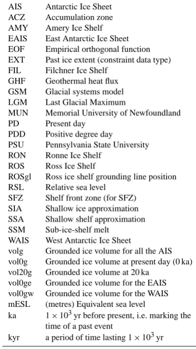
Table 1. Table of abbreviations.

AIS Antarctic Ice Sheet

ACZ Accumulation zone

AMY Amery Ice Shelf

EAIS East Antarctic Ice Sheet

EOF Empirical orthogonal function

EXT Past ice extent (constraint data type)

FIL Filchner Ice Shelf

GHF Geothermal heat flux

GSM Glacial systems model

LGM Last Glacial Maximum

MUN Memorial University of Newfoundland

PD Present day

PDD Positive degree day

PSU Pennsylvania State University

RON Ronne Ice Shelf

ROS Ross Ice Shelf

ROSgl Ross ice shelf grounding line position

RSL Relative sea level

SFZ Shelf front zone (for SFZ)

SIA Shallow ice approximation

SSA Shallow shelf approximation

SSM Sub-ice-shelf melt

WAIS West Antarctic Ice Sheet

volg Grounded ice volume for all the AIS vol0g Grounded ice volume at present day (0 ka) vol20g Grounded ice volume at 20 ka

vol0ge Grounded ice volume for the EAIS vol0gw Grounded ice volume for the WAIS mESL (metres) Equivalent sea level

ka 1×103yr before present, i.e. marking the time of a past event

kyr a period of time lasting 1×103yr

considered together, creates a phase space of possible recon-structions. More complex models invariably have more pa-rameterizations and a larger phase space.

With a handful of ensemble parameters, the traditional method of hand-tuning models with a small number of runs (O(10)) is restrictive and limits exploration of the parameter space. Depending on the non-linearity of the system and the number of parameters, even the generation of relatively large ensembles (O(103–104)) is likely far from adequate. As well, with such large numbers of model runs, an objective and sys-tematic means to quantify run quality is critical.

The plausibility of each model run can be assessed by comparisons against observations. Thus, each run can be evaluated in relation to its misfit to the observational data, and a “misfit score” can be attributed allowing runs to be ranked. Runs can then be combined (for example as weighted averages, using the scores as weights) to produce compos-ite deglaciation chronologies. In addition, by capturing the observational, parametric, and structural uncertainties and propagating them into the evaluation process, the cumulative uncertainties can be computed and presented along with the

reconstructions (Briggs and Tarasov, 2013). This developing approach has already been applied to other major Quaternary ice sheets (Tarasov and Peltier, 2003, 2004; Tarasov et al., 2012).

This model description and sensitivity assessment paper is one in a suite of three articles documenting the steps under-taken to produce a data-constrained deglaciation chronology, with associated uncertainties, for the AIS using a large en-semble analysis approach (3000 or more runs per enen-semble). The second article presents a database of observational data and describes a method that can be employed to quantita-tively evaluate model output using the constraint data (Briggs and Tarasov, 2013). The generation of the ensemble and sub-sequent analysis of the generated chronologies is described in Briggs et al. (in preparation).

The Memorial University of Newfoundland/Penn State University (MUN/PSU) model has been developed specifi-cally for ensemble analysis of AIS deglaciation. The dynam-ical core of MUN/PSU is based on the Penn State University 3-D ice sheet model (Pollard and DeConto, 2007; Pollard and DeConto, 2009; Pollard and DeConto, 2012b). In this paper we document how MUN/PSU differs from the PSU model and describe 31 ensemble parameters used to explore a set of uncertainties in the glacial systems model (GSM). We also assess model sensitivity to parameter variations.

2 Model description and spin-up

The ice dynamical core of the MUN/PSU model is the PSU 3-D ice sheet model (Pollard and DeConto, 2012b, and refer-ences therein). The original PSU model was developed for continental scale applications over long (up to O(106)yr) periods. It has been used in many studies for the AIS and other ice sheets (see Pollard and DeConto, 2012b, for a com-plete list) over a range of spatial and temporal scales and has generally performed well within the range of other models in the ISMIP-HEINO, ISMIP-HOM, and MISMIP intercom-parison tests (Calov et al., 2010; Pattyn et al., 2008, 2012).

The key features of the MUN/PSU GSM are (items marked with an asterisk deviate significantly from the PSU model) the following:

– treatment of both shallow ice and shallow shelf/stream

regimes, including a parameterization based on Schoof (2007) boundary layer theory

– a standard coupled thermodynamic solver including

horizontal advection, vertical diffusion and heat gen-erated from deformation work

(3)

– ∗_{visco-elastic isostatic adjustment (bedrock response}

to surface loading) component

– ∗parameterized climate forcing that generates three separate temperature and precipitation fields concur-rently, which are subsequently merged, through further ensemble parameters, to produce a final “blended” set of climate fields (developed to avoid dependence on a single climate forcing parameterization)

– ∗parameterizations for the separate treatment of tide-water and ice shelf front calving

– ∗_{a new physically motivated empirical approach to}

sub-ice-shelf melt (SSM)

We expose underlying GSM uncertainties (inevitably to an incomplete extent) through a synthesis of previous pa-rameterizations from the literature with a focus on making explicit at least some of the underlying parametric sensitiv-ities. Their validation stems from a combination of the doc-umented source origin, physical plausibility/motivation, and resultant impact on characteristics/statistics of generated ice sheet chronologies.

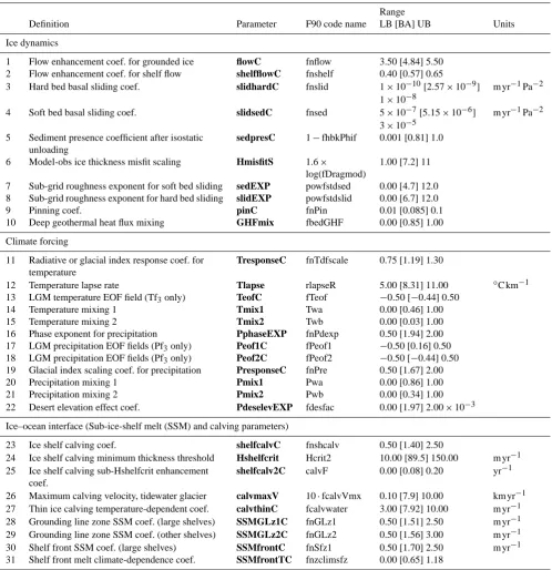
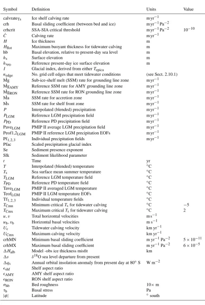
The 31 ensemble parameters in the GSM are summarized in Table 2. They are listed in the order they are discussed in the text and organized in accordance with the model func-tionality they affect: ice dynamics (10 parameters), climate forcing (12 parameters) and ice–ocean mass loss through calving and sub-ice-shelf melt (9 parameters). The evolu-tion of the parameter range and justificaevolu-tions for choos-ing/excluding parameters are discussed in greater detail in Sect. 3. The ranges presented in Table 2 contains three val-ues, the upper bound, the value of the parameter from a base-line run, and the lower bound. The basebase-line run is used and discussed fully in the sensitivity assessment (Sect. 3). The baseline run has one of the smallest misfit-to-observation scores of runs to date as identified through the application of the constraint data and the evaluation scheme (Briggs and Tarasov, 2013). Table 3 provides a full list of all the variables and non-ensemble parameters discussed in the text.

2.1 Model setup

We adopt the same discretization methodology as the PSU model (Pollard and DeConto, 2009, 2012b). In summary, for the context of our large ensemble-based analysis, the MUN/PSU model is run at a resolution of 40 km in the hori-zontal direction and uses a finite-difference Arakawa-C grid. In the vertical the grid has 10 uneven layers, spaced closer at the surface and base of the ice. The horizontal velocitiesu, v are located between the grid points (i.e. staggered half a grid cell), whereas the ice geometry (e.g. ice thicknessH, sur-face elevationhs), vertical velocities, and temperatures are located at the grid centres. A comparison of results for the PSU model at 40, 20 and 10 km resolutions are shown in Fig. 6 of Pollard and DeConto (2012b) and Appendix C of

Pollard and DeConto (2012a), with very little difference in computed modern ice distributions. The primary model fea-ture that allows this insensitivity to resolution is the ground-ing line flux parameterization of Schoof (2007), as discussed in the above two references.

The standard model run is from 205 ka to present day (the initialization conditions are described in Sect. 2.11). The model has adaptive time-stepping functionality that, if numerical instabilities occur, enables the GSM to revert to a previous state (the state is recorded by a rolling buffer) and re-attempt the calculations with reduced time steps (50 % reduction upon each reversion). After 300 yr under reduced time step conditions, the time step is doubled. On initializa-tion the ice dynamics are set to be computed every 0.5 yr, thermodynamics every 10 yr, and isostatic adjustment every 100 yr.

2.2 Ice dynamics

Grounded and floating ice have the same fundamental rheol-ogy, but the large-scale (simplified) equations that describe them are different. Three regimes classify the type of ice flow: sheet flow, stream flow and shelf flow. Sheet flow, under the zero-order shallow-ice approximation (SIA), is valid for an ice mass with a small aspect ratio (height scalelength scale) and where the flow is dominated by vertical shear stress, i.e. much of the interior of the AIS. It is the sim-plest type of flow. The driving stress is in balance with basal traction (the retaining force due to friction at the interface between an ice sheet and the underlying bed). The flow is dominated by vertical shear (∂u/∂z, whereuis velocity and z is the vertical co-ordinate within the ice thickness) de-termined locally by the driving stress. The driving stress is a function of the surface gradient and the thickness; steeper slopes and/or thicker ice beget larger driving stresses. In shal-low shelf fshal-low (SSA), the driving stress is balanced by lon-gitudinal and transverse (horizontal) shear stress gradients. Stream flow is similar to shelf flow, except for the presence of basal drag, and the basal topographic boundary condition (MacAyeal, 1997).

(4)

Table 2. Ensemble parameters. LB = lower bound, BA = baseline and UB = upper bound. Values are rounded to 2 decimal places.

Range

Definition Parameter F90 code name LB [BA] UB Units

Ice dynamics

1 Flow enhancement coef. for grounded ice flowC fnflow 3.50 [4.84] 5.50

2 Flow enhancement coef. for shelf flow shelfflowC fnshelf 0.40 [0.57] 0.65

3 Hard bed basal sliding coef. slidhardC fnslid 1×10−10[2.57×10−9] m yr−1Pa−2

1×10−8

4 Soft bed basal sliding coef. slidsedC fnsed 5×10−7[5.15×10−6] m yr−1Pa−2

3×10−5 5 Sediment presence coefficient after isostatic

unloading

sedpresC 1−fhbkPhif 0.001 [0.81] 1.0

6 Model-obs ice thickness misfit scaling HmisfitS 1.6× 1.00 [7.2] 11

log(fDragmod)

7 Sub-grid roughness exponent for soft bed sliding sedEXP powfstdsed 0.00 [4.7] 12.0

8 Sub-grid roughness exponent for hard bed sliding slidEXP powfstdslid 0.00 [6.7] 12.0

9 Pinning coef. pinC fnPin 0.01 [0.085] 0.1

10 Deep geothermal heat flux mixing GHFmix fbedGHF 0.00 [0.85] 1.00

Climate forcing

11 Radiative or glacial index response coef. for temperature

TresponseC fnTdfscale 0.75 [1.19] 1.30

12 Temperature lapse rate Tlapse rlapseR 5.00 [8.31] 11.00 ◦C km−1

13 LGM temperature EOF field (Tf3only) TeofC fTeof −0.50 [−0.44] 0.50

14 Temperature mixing 1 Tmix1 Twa 0.00 [0.46] 1.00

15 Temperature mixing 2 Tmix2 Twb 0.00 [0.03] 1.00

16 Phase exponent for precipitation PphaseEXP fnPdexp 0.50 [1.94] 2.00

17 LGM precipitation EOF fields (Pf3only) Peof1C fPeof1 −0.50 [0.16] 0.50

18 LGM precipitation EOF fields (Pf3only) Peof2C fPeof2 −0.50 [−0.44] 0.50

19 Glacial index scaling coef. for precipitation PresponseC fnPre 0.50 [1.67] 2.00

20 Precipitation mixing 1 Pmix1 Pwa 0.00 [0.86] 1.00

21 Precipitation mixing 2 Pmix2 Pwb 0.00 [0.34] 1.00

22 Desert elevation effect coef. PdeselevEXP fdesfac 0.00 [1.97] 2.00×10−3

Ice–ocean interface (Sub-ice-shelf melt (SSM) and calving parameters)

23 Ice shelf calving coef. shelfcalvC fnshcalv 0.50 [1.40] 2.50

24 Ice shelf calving minimum thickness threshold Hshelfcrit Hcrit2 10.00 [89.5] 150.00 m yr−1

25 Ice shelf calving sub-Hshelfcrit enhancement coef.

shelfcalv2C calvF 0.00 [0.08] 0.20 yr−1

26 Maximum calving velocity, tidewater glacier calvmaxV 10·fcalvVmx 0.10 [7.9] 10.00 km yr−1

27 Thin ice calving temperature-dependent coef. calvthinC fcalvwater 3.00 [7.92] 10.00 m yr−1

28 Grounding line zone SSM coef. (large shelves) SSMGLz1C fnGLz1 0.50 [1.51] 2.50 m yr−1

29 Grounding line zone SSM coef. (other shelves) SSMGLz2C fnGLz2 0.50 [1.56] 3.00 m yr−1

30 Shelf front SSM coef. (large shelves) SSMfrontC fnSfz1 0.50 [1.70] 2.50 m yr−1

31 Shelf front melt climate-dependence coef. SSMfrontTC fnzclimsfz 0.00 [0.65] 1.18

(Pollard and DeConto, 2007, 2012b). Significant savings in CPU time, with virtually no impact on the results, can be earned by limiting the combined SIA-SSA equations to cells where SSA flow is predisposed to dominate due to low basal drag; above a critical threshold (satisfied in the majority of the East Antarctic Ice Sheet (EAIS)) the flow is limited to SIA (Pollard and DeConto, 2009). Further reductions in com-puting resource can be achieved by removing the SIA

(5)

Table 3. Table of symbols and (non-ensemble) model parameters discussed in the text.

Symbol Definition Units Value

calvrateTs Ice shelf calving rate m yr−1

crh Basal sliding coefficient (between bed and ice) m yr−1Pa−2

crhcrit SSA-SIA critical threshold m yr−1Pa−2 10−10

˙

C Calving rate m yr−1

H Ice thickness m

Hflot Maximum buoyant thickness for tidewater calving m

hb Basal elevation, relative to present-day sea level m

hs Surface elevation m

hsPD Reference present-day ice surface elevation m

I Glacial index, derived from eitherTepica

nedge No. grid cell edges that meet tidewater conditions (see Sect. 2.10.1)

˙

Mg Sub-ice-shelf melt (SSM) rate for grounding line zone m yr−1

˙

Mg_AMY Reference SSM rate for AMY grounding line zone m yr−1

˙

Mg_RON Reference SSM rate for RON grounding line zone m yr−1

˙

Ma SSM rate for accretion zone m yr−1

˙

Ms SSM rate for shelf front zone m yr−1

P Interpolated (blended) precipitation m yr−1

PLGM Reference LGM precipitation field m yr−1

PPD Reference PD precipitation field m yr−1

PaveLGM PMIP II average LGM precipitation field m yr−1

Peof1,2LGM PMIP II reference LGM precipitation EOFs m yr−1

Pf1,2,3 Individual precipitation fields m yr−1

Pfac Scaled precipitation glacial index

Se Sediment presence exponent

Slk Sediment likelihood parameter

t Time yr

T Interpolated (blended) temperature ◦C

Ts Sea surface mean summer temperature ◦C

TLGM Reference LGM temperature field ◦C

TPD Reference PD temperature field ◦C

TaveLGM PMIP II averaged LGM temperature ◦C

Teof_LGM PMIP II LGM temperature EOFs ◦C

Tf1,2,3 Individual temperature fields ◦C

TCmn Minimum criticalTsfor tidewater calving ◦C −5

TCmx Maximum criticalTsfor tidewater calving ◦C 2

u, v Total horizontal velocities m s−1

ub, vb Horizontal basal velocities m s−1

Uc Tidewater calving velocity km yr−1

UCmx Maximum calving velocity km yr−1

crhMN Minimum basal sliding coefficient m yr−1Pa−2 5×10−11

crhMX Maximum basal sliding coefficient m yr−1Pa−2 6×10−5

1Halb Model -obs ice thickness misfit km

1s δ18O sea level departure from present

1qs Annual orbital insolation anomaly from present day at 80◦S W m−2

shf Shelf aspect ratio

AMY AMY shelf aspect ratio

RON RON shelf aspect ratio

σhb Bed roughness 10×m

τb Basal stress Pa

(6)

order 3000 runs; each run can take 2–5 days on a single pro-cessor core), the latter method is employed for this study.

2.3 Ice rheology factor

The sheet and shelf flow enhancement ensemble parameters,

flowC and shelfflowC1, multiplicatively adjust the ice

rheol-ogy (Pollard and DeConto, 2012b, Eqs. 16a and 16b). They are motivated as providing softening due to the unresolved grain-scale characteristics (e.g. ice crystal size, orientation, impurities) of the ice (Cuffey and Paterson, 2010, p. 71). En-hancement factors are between 3.5 and 5.5 for sheet flow and between 0.4 and 0.65 for shelf flow. This approximately fol-lows the bounds defined in Ma et al. (2010). Physically they manifest themselves as a control on the height-to-width ratio of the ice sheet (Huybrechts, 1991).

2.4 Basal drag

Though a consensus is developing towards the validity of Coulomb plastic basal drag from subglacial sediment defor-mation (Cuffey and Paterson, 2010), the Schoof grounding line flux condition (Schoof, 2007) is only defined for power law forms. We therefore retain the warm-based basal drag parameterization of Pollard and DeConto (2007, 2012b),

ub=crh·τb2, (1)

whereubis the basal sliding velocity, crh is the basal sliding coefficient, andτbis the basal stress. The basal drag parame-terization is written in an inverted basal sliding form to pro-vide a conceptually simpler linear relationship between crh and basal velocity. Once the non-linearity of the ice system is factored in, the proportionality will, however, cease to be linear. Runs with ensemble parameters that generate larger values of crh will generally have increased basal velocities, but this is unlikely to hold everywhere at every time. A fu-ture study will examine model sensitivity to the form of basal drag law (i.e. including the value of the exponent, replace-ment with a Coulomb plastic relationship, and inclusion of full coupling with basal hydrology).

To capture the large uncertainty in subglacial basal stress regimes, we have introduced a number of ensemble parame-ters that are used to determine the basal sliding coefficient.

Firstly, following Pollard and DeConto (2012b), we con-sider the local bed to be either hard or soft (sediment) bed dominated. These two regimes have corresponding ensemble parameters: slidhardC (1×10−10 to 1×10−8m yr−1Pa−2, predominantly under the EAIS) and slidsedC (5×10−7 to 3×10−5m yr−1Pa−2, predominantly under the WAIS).

The parameterization has three key dependencies. First, as per Pollard and DeConto (2012b), we assume that the dis-tribution of subglacial sediment is largely related to the sur-face elevation of the unloaded subglacial topography. Areas

1_{All ensemble parameter names are boldfaced.}

that are still submerged after glacial unloading are likely to have soft sedimentary surface lithology, and therefore are a precursor for subglacial sediment. With some allowance for uncertainty in the resultant unloaded surface elevation (dependent on present-day ground surface elevation and ice thickness, and thus uncertainty in ALBMAP(LeBrocq et al., 2010), earth rheology, subglacial erosion rates, etc.) under the control of a parameter sedpresC (0.001–1), we define a sediment likelihood parameter

Slk=unloaded water depth in km

sedpresC . (2)

The sedpresC parameter can arguably be interpreted as an allowance for an uncertain amount of erosion since initial glaciation that would otherwise bias the inference of long-term marine submergence prior to glacial loading. We use Slk to set a sediment presence exponent, Se, that controls the transition from slidhardC to slidsedC (bare rock to sed-iment):

Se=

  

 

1,if Slk>1 unloaded marine: thick sediment cover Slk, if 0≤Slk≤1 some sediment

0,if Slk<0 unloaded terrestrial: no sediment.

(3)

The second dependence is on sub-grid roughness, given by the standard deviation (σhb, in dekametres) of the 5 km-resolution ALBMAP (LeBrocq et al., 2010)2 basal topog-raphy for each GSM grid cell. For Antarctic and associ-ated ice shelves, σhb ranges from 0.16 to 2.4 with an un-weighted mean value of 0.80. For regions with thick sed-iment cover (Se>0.67), we assume that higher roughness will lead to increased basal drag. For minimal or no sediment cover (Se<0.5), we assume that enhanced surface rough-ness increases the surface area available to erosion, promot-ing trapppromot-ing of eroded sediments, leadpromot-ing to reduced basal drag. For consistency of the above logic, any site with sedi-ment cover should have reduced basal drag compared to sites without sediment cover. Below we detail one way to enforce this consistency, but it is not implemented in the results pre-sented herein.

The final dependence takes into account the local ice thick-ness difference1Halbbetween the present-day field from a best-fitting test run from a previous ensemble and ALBMAP thickness HALB (in km). Thus we address some observa-tion model misfit in the adjustment of crh and perhaps par-tially compensate for weaknesses in the assumptions of the 2_{The ALBMAP dataset is provided at a resolution of 5 km. To}

(7)

first two dependencies. This is a similar, albeit much sim-pler, approach to the local inverse method employed by Pol-lard and DeConto (2012a) to adjust the values of crh to re-duce model misfit. The HmisfitS (range 0.0–11.0) ensem-ble parameter scales the exponential sensitivity to1Halb, so that for1Halb>0 (i.e. test run ice thickness in excess of ALBMAP) the parameterization results in a larger value of crh and therefore increased basal velocities and reduced basal drag.

The basal sliding coefficient crh is set as

crh=F (Tb)·max "

min "

slidhardC

_slidsedC

slidhardC

Se (4)

·fstd·exp((HmisfitS·1Halb)),crhMX

,crhMN

,

whereF (Tb) nominally denotes the temperature dependence for the cold-to-warm-based transition detailed below. Model parameters crhMX and crhMN set the respective warm-based upper and lower bounds for crh. The bed roughness depen-dency (fstd) in the above expression for crh is given by

if Se>0.67 then Fthicker sediment

ifσhb≥0.75 then F rougher sub-grid topography fstd=max

(0.75/σhb)sedEXP, 0bnd Fdecreased sliding

else F smoother sub-grid topography

fstd=(1+(0.75−σhb)/0.69)sedEXP

end if Fincreased sliding

else if Se<0.5 then Fthinner sediment fstd=minσ_hbslidEXP, 0bnd Fsliding increased for

else rough topography

fstd=1 end if.

For the results presented below,0bndis inactive (e.g. set to 0 for σhb≥0.75 and 105 otherwise). To enforce that fstd never induces overlap of crh values between hard (Se< 0.5) and soft bed (Se≥0.5) ranges, one choice is that which sets crh to the geometric mean of slidsedC and

slid-hardC (0bnd=(slidsedC/slidhardC)(0.5−Se)). However,

other choices are also plausible, and one could therefore ar-gue for the introduction of another ensemble parameter to set the value of0bnd. Future work will use a high-resolution, higher-order ice sheet model to develop a better constrained accounting of the impact of sub-grid topography on ice flow and basal motion for continental-scale glacial-cycle mod-elling where mountain resolving resolution is not feasible.

High sub-grid topographic roughness is also likely to en-tail significant sub-grid variation in basal temperature rel-ative to the pressure melting point. Our sliding coefficient parameterization above is inactive for regions that are cold-based, and therefore the effective basal drag may be overes-timated in these regions. Pollard and DeConto (2012b) pa-rameterized an allowance for this effect that will be

consid-ered for future model upgrades (again after a high-resolution model comparison).

As shown in Supplement Fig. 1, ensemble parameters

HmisfitS, slidEXP, sedEXP, slidhardC and slidsedC

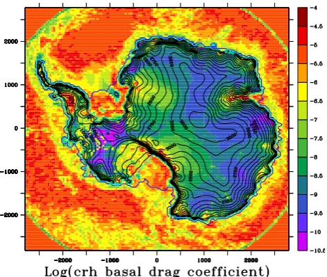
per-mit a wide range of basal sliding coefficients in response to variations in1Halbandσalb. Aside from the above-described dependencies and the constraints of appropriate scale re-sponse (which motivated some of the power terms) and nu-merical continuity, the exact form of the above drag coeffi-cient equations developed in a somewhat ad hoc trial-and-error approach. For instance, the values in the second fstd relationship above (i.e. for Se>0.67 and Se<0.75) were constrained by continuity and a decision to make the maxi-mum value of fstd=2sedEXP. For the case of the slidEXP and sedEXP = 1, the above equation gives fstd a range of [0.167–2] for Se>0.67 and [1–4.5] for Se<0.5. The en-semble parameters sedEXP and slidEXP both have ranges of 0:12. Numerical coefficients were selected from initial sensi-tivity analyses while maintaining numerical continuity. An example basal sliding coefficient field is shown in Fig. 1. Values of log(crh) below−8.59 in the figure are due to the

exp((HmisfitS·1Halb))factor in Eq. (4).

It may be that the parameter ranges of slidsedC and

slid-hardC will turn out to be physically untenable. However, at

this stage, we deem errors from inadequate parameter range coverage of more concern. Deleting results with untenable parameter values in the future is much less costly than hav-ing missed a sector of the potential parameter space that bet-ter corresponds to “reality”.

Mass fluxes for grounded ice with basal sliding coeffi-cient crh>crhcrit=10−8_{m yr}−1_Pa−2_{are determined by the} combined SSA and SIA equations; otherwise only SIA is ac-tive. At the cold-to-warm-based transition, crh smoothly in-creases in value from an essentially zero (10−20m yr−1Pa−2) value starting at basal temperature−0.5◦C below the pres-sure melting point. The temperature coefficient, F (Tb), in Eq. (4) implements an exponential transition that reaches a maximum value of one at the pressure melting point, except at the grounding line where a warm base (i.e.F (Tb)=1) is always imposed.

2.5 Grounding line treatment

At the locality of the grounding line and in ice streams with very little basal traction, a combination of both ice sheet and ice shelf flow regimes exists (Pollard and DeConto, 2007).

(8)

Fig. 1. Basal sliding coefficient for baseline parameter vector nn2679 and associated surface elevation contours. Note value re-ductions due to cold basal conditions have not been applied to the plotted field. The logarithms of slidhardC and slidsedC have re-spective values−8.5886 and−5.2881.

at the grounding line, and the sliding coefficient discussed above (Schoof, 2007). The longitudinal stress is calculated by the stress balance equation and also takes into account back stress at the grounding line caused by buttressing from pinning points, downstream islands or side shear at lateral margins.

The analytically calculated ice fluxqg and height at the grounding line Hg, found through linear interpolation, are then used to compute the depth-averaged velocity at the grounding lineug=qg/Hg. The calculatedugis imposed as an internal boundary condition for the shelf-flow equations and is used to overwrite the velocity solution calculated for that position from the stress balance equations (Pollard and DeConto, 2007, 2012b).

2.6 Sub-ice-shelf pinning points

Pinning points, sometimes manifest in the form of small ice rises, are found below the ice shelves, generally toward the grounding line. Grounding of the ice shelf onto such pinning points causes additional back stresses that influence the mi-gration of the grounding line (Pollard and DeConto, 2012b). These pinning points are too small to be resolved on a 40 km grid, and the pinning point drag is therefore parameterized to be a fraction of the equivalent basal drag for grounded ice as a function of the water depth. Ensemble parameter

pinC (range 0.01–0.1) scales the computed pinning point

drag by assuming that the fraction of grounded ice is given by max0.,min(1.,1.−(hw/300.))

×pinC, wherehwis the

water depth (m) and coefficients are taken from Pollard and DeConto (2009).

2.7 Isostatic adjustment and relative sea level

computation

The isostatic adjustment component of the GSM is taken from Tarasov and Peltier (2004) but modified to use the VM5a earth rheology of Peltier and Drummond (2008) which still retains a 90 km-thick elastic lithosphere. The visco-elastic earth rheology is spherically symmetric and has reasonable fits to geophysical observations from North America (Peltier and Drummond, 2008). The bedrock dis-placement is computed every 100 yr from a space–time con-volution of surface load changes and a radial displacement Greens function, at spherical harmonic degree and order 256. This study considers the glaciological and climatic un-certainties in the GSM, but assessment of the contribution from rheological uncertainties is a future project. For a pre-liminary examination of the impact of Earth model uncer-tainty on inferred Antarctica deglacial history see White-house et al. (2012). Variations (within bounds from geophys-ical constraints) in the earth rheology will have some impact on ice evolution, but that will get swamped by the other un-certainties, e.g. the climate forcing.

2.8 Geothermal heat flux (GHF)

There are very few direct measurements of GHF for the AIS. Those that do exist are usually derived from direct temper-ature measurements in ice cores (Pattyn, 2010). As such, continental scale GHF reconstructions must be derived from proxies. This study employs two GHF datasets which are linearly blended through ensemble parameter GHFmix. The Shapiro and Ritzwoller (2004) dataset uses a global seismic model of the crust and upper mantle to extrapolate avail-able measurements to regions where they are non-existent or sparse. The Fox Maule et al. (2005) dataset was esti-mated from satellite-measured magnetic data. The GHF field in the model linearly ranges from the former (GHFmix = 1) to the latter (GHFmix = 0) dataset. The datasets are cor-rected, around a Gaussian area of influence, so that the recon-structions match the observations where available (Pattyn, 2010). The observations are derived from ice core temper-ature profiles and based on the location of sub-glacial lakes (the ice/bedrock interface can then be considered to be at the pressure melting point, and thus the minimum GHF can be computed; Pattyn, 2010).

2.9 Climate forcing

(9)

different parameterizations, each of which has one or more ensemble parameters, are used to concurrently generate the temperature (Tf1,2,3) and precipitation (Pf1,2,3) fields.

The spatial distribution of the fields is obtained through empirical parameterizations, from published observational datasets (e.g. Arthern et al., 2006), or for Tf3from the Paleo-Modelling Intercomparison Project II (PMIP II; Braconnot et al., 2007) modelling study.

The fields are then projected backwards in time using an ice or deep-sea core time series (Ritz et al., 2001; Huy-brechts, 2002; Tarasov and Peltier, 2006; Pollard and De-Conto, 2009). Finally, the different fields are combined using a weighed sum, the weight determined by ensemble parame-ters, to generate the final climate fields that force the GSM.

This approach ensures there is no reliance on a single cli-mate methodology and that each method has one or more ensemble parameters. This affords the model a larger degree of freedom (with respect to climate forcing) than the single climate forcing methodology with limited parameterization employed in other studies (e.g. Pollard and DeConto, 2012b; Whitehouse et al., 2012).

2.9.1 Temperature forcing

Tf1models the spatial variation of the temperature field as a function of latitude, height, and lapse rate with coefficients from Martin et al. (2011) and sea level dependence from Pol-lard and DeConto (2009). Using the annual orbital insola-tion anomaly (1qs) at 80◦S (W m−2) and sea level departure from present (1s), the modern-day temperature field is ad-justed to generate a palaeo-temperature field. Annual orbital insolation is calculated from Laskar et al. (2004) and, follow-ing Tarasov and Peltier (2004), it is weighted by ensemble parameter TresponseC (range 0.75–1.3) to account for the uncertainty inherent in using this method to drive the tran-sition between a glacial and interglacial state. The sea level departure from present is taken from stacked benthicδ18O records (Lisiecki, 2005). Present-day Tf1is shown in Fig. 3a of the Supplement. This field is computed in degrees Celsius as

Tf1(x, t )=30.7−0.0081hs(x, t )−0.6878|8(x)| (5) +0.1 TresponseC·1qs(t )+

1s(t ) 12.5 ,

wherehs is modelled surface height (m, relative to present-day sea level), and8is latitude (◦). To avoid overly low tem-peratures over the ice shelves, we follow Martin et al. (2011) and remove the dependence on surface elevation when it is below 100 m,

Tf1(x, t )=29.89−0.6878|8|+0.1TresponseC·1qs(t ) (6) whenhs(x, t ) <100 m.

The second temperature forcing field, Tf2 (Supplement Fig. 3b), is distinguished from Tf1by the use of the Comiso (2000) present-day surface air temperature map (available

as part of ALBMAP) for the AIS (TPD), removal of sea level dependence, and the inclusion of an adjustable vertical temperature gradient via the ensemble parameter lapse rate (Tlapse). The lapse rate range is 5–11◦C km−1(compared with, for example, 9.14◦C km−1; Ritz et al., 2001; Pollard and DeConto, 2009 and 8.0◦C km−1; Pollard and DeConto, 2012b). Then,

Tf2(x, t )=TPD(x)+0.1 TresponseC·1qs (7)

+Tlapse

hs(x, t )−hsPD(x)

where1qsandhsare as for Tf1.

Following Tarasov and Peltier (2004), Tf3 is calculated by interpolating between PD surface temperature (Comiso, 2000) and a Last Glacial Maximum (LGM) air surface temperature field generated from an amalgam of the re-sults of five high-resolution PMIP II (Braconnot et al., 2007) 21 ka simulations (CCSM, HadCM3M2, IPSL-CM4-V1-MR, MIROC3.2 and ECHAM53). The 5 datasets are av-eraged together (TaveLGM) and we also use the first empirical orthogonal basis function (EOF) of inter-model variance for the LGM snapshots3. The first EOF (TeofLGM) captures 64 % of the total variance and is incorporated through ensemble parameter TeofC (range−0.5–0.5) into a run-specific LGM reference temperature fieldTLGM when the model is initial-ized,

TLGM(x)=TaveLGM(x)+TeofC·TeofLGM(x). (8) The computed TaveLGM and the associated TeofLGM are shown in Supplement Fig. 4. As with Tf2, the present-day and LGM temperature fields are adjusted, through the pa-rameterized lapse rate, to account for the difference between the modelled surface elevation,hs, and the reference surface elevation fields hsPD andhsLGM (the PMIP II files are sup-plied with an associated LGM orthography). The interpo-lation between the Comiso (2000) present-day temperature field and the model-derived LGM temperature is weighted using a glacial index,I, derived from the EPICA tempera-ture recordTepica(Jouzel and Masson-Delmotte, 2007), I (t )= Tepica(t )−Tepica(0)

Tepica(LGM)−Tepica(0)

, (9)

and adjusted using ensemble parameter TresponseC giving Tf3(Xt, t )=TPD(x)+Tlapse·(hs(x, t )−hsPD(x)) (10)

·(1−(TresponseC·I (t ))

+TLGM(x)+Tlapse·(hs(x, t )−hs_LGM(x))

·(TresponseC·I (t )).

3_{This is a numerical technique to decompose in this case the}

(10)

As compared to the time-dependence of Tf1, the I (t ) glacial index (cf. Supplement Fig. 2) has more high-frequency variability along with a tendency to a pre-LGM cold-bias except for a stronger warming during the Eemian. The three temperature fields are then combined in accor-dance with two ensemble parameters, Tmix1 and Tmix2 (both range 0–1), to produce the final temperature field, T (x, t )=(1−Tmix2)·_[Tmix1·Tf1(x, t ) (11)

+(1−Tmix1)·Tf2(x, t )]+Tmix2·Tf3(x, t ).

The extra weight given to Tf3 in the above was chosen on the basis of simplicity and the much more similar temporal dependencies (mostly via orbital insolation anomalies) of Tf1 and Tf2.

2.9.2 Precipitation forcing

The precipitation forcing is also subject to a weighted amal-gam of three different forcings. Pf1assumes precipitation is driven by temperature (as per Huybrechts et al., 1998), Pf1(x, t )=1.5×2T (x,t )10−Tm_. ₍₁₂₎ whereT is the blended temperature andTmis 0◦C. This re-lationship is motivated by the exponential dependence of the saturation vapour pressure on temperature. Present-day Pf1 is shown in Supplement Fig. 3c.

Pf2is computed in a similar manner to Tf2; at run-time, an observational dataset,PPD(shown in Supplement Fig. 3d), of present-day precipitation (Arthern et al., 2006) is adjusted us-ing the annual orbital insolation anomaly. Ensemble param-eter PphaseEXP (range 0.5–2) accounts for some response uncertainty to the insolation anomaly,

Pf2(x, t )=PPD(x)×2PphaseEXP1q100s(t )_. ₍₁₃₎ In a similar manner to Tf3, Pf3 is computed using the glacial index I (t ) to interpolate between the present-day datasetPPDand an LGM precipitation field, generated from an amalgam of the PMIP II LGM precipitation simulations, PaveLGM. Two EOFs are used. The first (Peof1) captures 62 % of the inter-model variance, the second (Peof2) captures 23 %. The computed PaveLGM and the associated EOF’s are plotted in Supplement Fig. 5. As with Tf3the EOFs are in-troduced at model initialization through parameters Peof1C and Peof2C (range−0.5–0.5) to create a run specific refer-ence dataset,

PLGM(x)=PaveLGM(x)+Peof1C·Peof1LGM(x) (14)

+Peof2C·Peof2LGM(x).

This is scaled and adjusted using ensemble parameter

Pre-sponseC (range 0.5–2),

Pf3(x, t )=PPD(x)

PresponseCPLGM(x)

PPD(x) Pfac

, (15)

where Pfac is the glacial index exponentially scaled by en-semble parameter PphaseEXP (range 0.5–2),

Pfac=sign [1.0, I (t )]|I (t )|PphaseEXP. (16) The final precipitation field is then summed and interpo-lated using two ensemble parameters Pmix1 and Pmix2, P (x, t )=qdes·((1−Pmix2)·[Pmix1·Pf1(x, t ) (17)

+(1−Pmix1)·Pf2(x, t )]+Pmix2·Pf3(x, t )) ,

whereqdesaccounts for the elevation-desert effect (reduced amount of moisture the atmosphere can hold at elevation) (Marshall et al., 2002; Tarasov and Peltier, 2004). It is sim-ulated as a function of the modelled elevation anomaly from present day,

qdes=exp−PdeselevEXP·(hs(x,t )−hsPD(x)), (18) and ensemble parameter PdeselevEXP (0–2×10−3).

The final “blended” temperature and precipitation fields are used to determine the fraction of precipitation that falls as snow and the annual surface melt. Given the small amount of surface melt over the AIS (Zwally and Fiegles, 1994), a sim-plified positive-degree-day method (PDD) is used with a melt factor of 5 mm PDD−1_.

2.10 Ice–ocean interface

The vast majority of mass loss from the AIS occurs from the ice shelves, either due to calving at the ice margin or from submarine melting beneath the ice shelf (Jacobs et al., 1992). The ice shelves play a crucial role in restricting (buttressing) the flow of ice (Dupont and Alley, 2005). Reduction or re-moval of the shelves allows the upstream grounded ice to ac-celerate, drawing down the ice in the interior. Thus, changes at the ice–ocean interface can have an impact hundreds of kilometres inland (Payne et al., 2004).

Iceberg calving has been inferred to be the largest con-tributor to mass loss. Jacobs et al. (1992) apportioned a loss of 2016 Gt yr−1 to calving against 544 Gt yr−1 to sub-ice-shelf melt (the uncertainty estimates for these numbers are large,±33 % for iceberg calving and±50 % for sub-ice-shelf melt). However, there is growing concern and evidence that the sub-ice-shelf melt rate is a primary control on the mass loss (Pritchard et al., 2012). Both processes are modelled in the GSM.

2.10.1 Calving

Marine ice margins can either terminate as a floating ice shelf or as a tidewater glacier. The GSM uses two distinct pa-rameterizations to calculate mass loss from either of these regimes; in addition there is an ad hoc treatment for thin ice.

Ice shelf calving

(11)

Fig. 2. SSM (sub-ice-shelf melt) implementation flowchart, with details for each distinct process zone: GLZ (grounding line zone), ACZ (accretion), and SFZ (shelf front).

9164

−25.00 −10.00 −5.00 −1.00 −0.50 −0.10 −0.01 0.01 0.10 0.50

Basal mass−balance rate (m/a)

9165

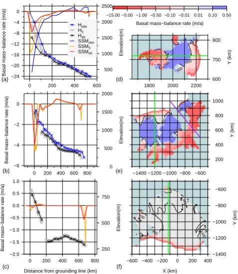
Fig. 3. Melt rate maps generated from lower (9164) and upper (9165) SSM parameter values. The large shelf regions are outlined in green (the latitude,8, and longitude,λ, boundaries are AMY=

8(−75,−65), λ(65,75) and 8(−75,−70), λ(75,80); ROS=

8(−86,−73), λ(160,210); RON=8(−85,−75), λ(280,313)

and FIL=8(−72,−85), λ(313,330)).

(e.g. Alley et al., 2008; Albrecht et al., 2011; Amundson and Truffer, 2010), we have found none to be stable for the rela-tively coarse grid of the GSM. For the present model config-uration, ice shelf calving is based on a steady-state approxi-mation of Amundson and Truffer (2010, Eq. 25) which corre-sponds to the insertion of the Sanderson (1979) relationship for ice shelf half-width into the empirical relation of Alley et al. (2008). Calving velocity is determined for each exposed face of the marginal grid cell. For a calving face normal to the xaxis, it is computed as

Uc= −H0˙xx _∂H

∂x −1

, (19)

−25 −20 −15 −10 −5 0 5

0 500 1000 1500 2000 2500

Ice thickness (m) AMY raw data

AMY pruned data AMY pruned quadratic fit to data

RON raw data RON pruned data RON pruned quadratic fit to data

ROS GLZ = 0.5*interpolated quadratic ROS GLZ = 1.0*interpolated quadratic ROS GLZ = 1.5*interpolated quadratic

(b) −25 −20 −15 −10 −5 0 5

0 500 1000 1500 2000 2500

Ice thickness (m)

0 100 200 300 400 500 600 700

Distance from grounding line (km)

(a)

AMY shelf thickness RON shelf thickness GLZ to ACZ (~700 m) AMY basal mass−balance RON basal mass−balance ACZ to SFZ (300−400 m)

(12)

250 500 750

Elevation(m)

0 200 400 600 800

Distance from grounding line (km) −2.0 −1.5 −1.0 −0.5 0.0 0.5 1.0

(c) (f) −1400 −1200 −1000 −800 −600 Y (km)

−600 −400 −200 0 200 400

X (km) 700 400 400 40 0 0 500 1000 1500 2000 Elevation(m)

0 200 400 600 800 −6

−4 −2 0

(b) (e) 200 400 600 800 1000 Y (km)

−1400 −1200 −1000 −800 −600

700 700 700 700 700 400 400 500 1000 1500 2000 2500 Elevation(m)

0 200 400 600 −24 −20 −16 −12 −8 −4 0

(a) (d) 600

700 800

Y (km)

1800 2000 2200 700 400 400 Hobs H5 H40 SSMobs SSM5 SSM40

−15.00 −5.00 −1.00 −0.50 −0.10 −0.01 0.01 0.10 0.50

Fig. 5. Transects of thickness and observed/computed melt rates, and computed spatial melt maps for the three major shelves: AMY (a, d), ROS (b, e), RON-FIL (c, f) computed from the SSM law with unity parameters (see text).Hobs, H5, and H40are the thicknesses

from the observed, ALBMAP5, and ALBMAP40datasets. SSMobs

is the observed melt rates. SSM5and SSM40are the computed melt

rates based on the respective ALBMAP thicknesses. Green line on the melt maps shows the locations of the transects. The purple line demarcates the divide between the FIL and RON shelves at 47◦W. The black contours highlight the observed 400 and 700 m thickness contours.

whereH0is the terminus ice thickness and˙xx is the along-flow spreading rate (soUc≥0). Due to the coarse grid reso-lution,˙xxand ∂H_∂x

−1

are computed one grid cell upstream from the terminus. The calving rate (ice loss per grid cell area,≥0), adjusted by ensemble parameter shelfcalvC (0.5– 2.5), is computed as

˙

C=shelfcalvC·Uc·

H0

1x. (20)

1x is the the terminal grid cell length perpendicular to the calving face. Once calculatedC˙ is used in the mass balance equation (Pollard and DeConto, 2012b, Eq. 14).

For ice thinner than 300 m the calving rate computed above is enhanced. Given the present-day correspondence between average ice shelf front and the mean annual−5◦C isotherm (Mercer, 1978), for ice thinner than 300 m and thicker than ensemble parameter Hshelfcrit (10–150 m), we impose a simple temperature-dependent (Ts, sea sur-face mean summer temperature in ◦C) parameterization.

For ice thinner than Hshelfcrit, calving is enhanced by a term shelfcalv2C·H, where ensemble parameter

shelf-calv2C ranges from 0 to 0.2 yr−1_{. Thus, the ice shelf calving}

rate is

˙

CIS=

     ˙

C, ifH≥300 ˙

C+max{(Ts+3◦)H₅◦·1 yr−1,0},if Hshelfcrit≤H <300 ˙

C+shelfcalv2C·H, ifH <Hshelfcrit.

(21)

The ad hoc nature of the above arose out of trial-and-error at-tempts to ensure a large range of calving response was attain-able. As for all the parameterizations presented herein, the judgement criteria is plausibility given current understanding and coverage of potential dynamical response over ensemble parameter ranges.

Tidewater calving

For grounded marine ice margins (i.e. large-scale tidewa-ter glaciers), we use a slight variant of the temperature-dependent proximity-to-flotation model of Tarasov and Peltier (2004). This parameterization is motivated by the proximity-to-flotation paradigm of tidewater calving (Van der Veen, 2002) along with an exponential temperature threshold to loosely account for the effects of sea ice and submarine melting, and the impact of surface water on crack propagation. Three conditions are imposed for such calving: (1) an adjacent ice-free grid cell with water depth greater than 20 m, (2) summer sea surface temperatureTs above a critical minimum valueTCmnand (3) ice thickness less than 1.15 times the maximum buoyant thickness,Hflot. When the above conditions are met, the calving velocity is given by

Uc=calvmaxV·min

" 1,

₁_.₁₅_H flot−H 0.35Hflot

2# (22) × exp ₃_·

(Ts−TCmx) TCmx−TCmn

(13)

0 50 100 150 200 250 300

Total mass loss (Gt/a)

Shelf

AMY ROS RON FIL OTHER

RON−F

IL

Jacobs, 1996 Wen, 2007 Yu, 2010 Loose, 2009 Joughin, 2003 (method 1) Joughin, 2003 (method 2) Grosfeld, 1998

H5 unity ensemble paramters

upper nn2679

unity ensemble paramters lower

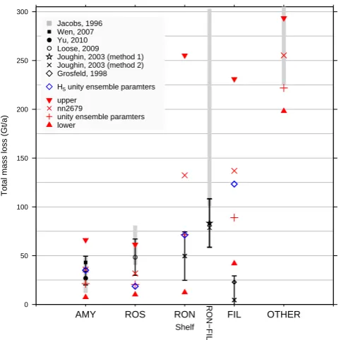
Fig. 6. Comparison plot showing net melt amounts from observa-tions and the predicted melt amount from the SSM component for each of the five shelf regions; two observations that are for the cu-mulative RON-FIL are also shown. The OTHER observation has been clipped as the maximum, estimated from Jacobs et al. (1996), peaks at 675 Gt yr−1(see Supplement Table 4).

Thin ice treatment

The ice shelf calving modules, and the sub-ice-shelf com-ponent described in the next section, were not designed for excessively thin (in this case<10 m thick) ice and we found it necessary to add a separate parameterization for this case. Again using the present-day correspondence between aver-age ice shelf front and the−5◦_{C isotherm (Mercer, 1978),}

we imposed a simple temperature-dependent parameteriza-tion. For marine ice<10 m thick, the calving rate is

˙ Cr=max

calving rate from other modules,0.3 (23)

+zclim(t )·calvthinC],

where calvthinC is a calibration parameter with a range 3– 10 m yr−1and zclim is an interglacial index factor (value 1 at 0 ka, value 0 at LGM, it is compared to other glacial in-dices presented above in Supplement Fig. 2). It is computed, as per Pollard and DeConto (2009), from the sea level depar-ture from present (1s) with some influence from the January orbital insolation anomaly (1qjan):

zclim(t )=max

0,min

1.5,1+1s(t )

85 (24)

+max

0,1qjan(t ) 40

.

Ice volume

0 50 100 150 200 250 300 350 400

Time (ka) high

low

Fig. 7. Lisiecki (2005) stacked benthicδ18O record as proxy for

global ice volume showing key times for spin-up run. For the gener-ation of the spin-up ensemble (see text for details), ice dynamics are only intermittently active from 391 kyr (red) until 205 kyr (green). For the ensemble proper, initialization starts at 205 kyr. Approxi-mate period of the Eemian is highlighted in grey.

2.10.2 Sub-ice-shelf melt

Sub-ice-shelf melt (SSM) is a reaction to a complex inter-action of oceanographic and glaciological conditions and processes. The newly developed SSM component used in MUN/PSU is a physically motivated implementation based on empirical observations. As such we provide a brief review of the SSM process to justify the implementation.

Three modes of melt have been identified (Jacobs et al., 1992). Mode 1 melt occurs in the grounding line zone of the larger shelves; driven by thermohaline circulation, it is triggered by the formation of high-salinity continental shelf water (HSSW). As sea ice forms near the ice shelf edge, brine rejection occurs, producing the dense HSSW. The wa-ter mass sinks and, upon reaching the continental shelf, drifts underneath the ice shelf into the grounding line cav-ity (the continental shelves generally slope down toward the grounding line due to long-term erosion by ice advances and to a lesser degree from isostatic depression). Due to the pressure dependence of the freezing point of water, the in situ melting point of the ice shelf base is lower than the temperature of the HSSW (formed at sea surface tempera-tures of e.g.∼ −1.9◦C). The encroaching water mass, act-ing as a heat delivery mechanism, melts away at the ice shelf base (Jacobs et al., 1992; Rignot and Jacobs, 2002; Joughin and Padman, 2003; Holland et al., 2008). The melt-ing ice freshens (and cools) the surroundmelt-ing water mass, pro-ducing buoyant ice shelf water (ISW), which, if not advected away, rises up and shoals along the base of the ice shelf. As the water mass rises the ambient pressure decreases, increas-ing the in situ freezincreas-ing point until refreezincreas-ing occurs, and new marine ice accretes onto the base of the ice shelf (Jacobs et al., 1992; Joughin and Padman, 2003).

(14)

et al., 2001). Grounding line melt rates of 31±5 m yr−1_have been estimated and accreted marine ice with a thickness up to 190 m have been calculated (Rignot et al., 2008; Fricker et al., 2001). ROS is the largest ice shelf by area but is much shallower with a draught of about 800 m; the melt rates are greatly reduced as is the marine ice accretion (∼10 m; Neal, 1979; Zotikov et al., 1980). RON and FIL both have deep grounding lines ∼1400 m and melt rates that can exceed 5 m yr−1 at some locations, the accreted marine ice can ex-ceed>300 m under RON, but, unlike AMY, it does not per-sist to the ice shelf front (Thyssen et al., 1993; Lambrecht et al., 2007).

Mode 2 and mode 3 melting occur both under the smaller shelves that fringe the AIS (e.g. those that face the Amund-sen, Weddell, and Bellingshausen seas) and proximal to the zone near the calving margin of the larger shelves. Mode 2 melting is associated with the intrusion of “warm” cir-cumpolar deep water (CDW) at intermediate depths (Ja-cobs et al., 1992; Ja(Ja-cobs et al., 1996; Joughin and Padman, 2003). The degree of melt is dependent on the amount of heat that can be delivered into the ice cavity, itself a func-tion of oceanographic condifunc-tions and the proximity of the ice base to the continental shelf edge. The highest melt rates oc-cur at the grounding lines of the Pine Island (44±6 m yr−1) and Thwaites (34±9 m yr−1) glaciers that discharge into the Amundsen Sea (Rignot and Jacobs, 2002). The grounding lines, at a depth of about 1000 m, are melted by the intru-sion of CDW water that is almost 4◦C above the in situ melting point (Rignot and Jacobs, 2002). Mode 3 melting is produced by seasonally warm surface water being advected against and underneath the ice shelf edge, through the action of tidal pumping and coastal currents (Jacobs et al., 1992). Melt rates of 2.8 m yr−1_{, decaying exponentially down to} zero around 40 km upstream from the calving margin, have been estimated for ROS. This is 10–40 % of the published total melt estimates for ROS (Horgan et al., 2011).

There is clear evidence that regional oceanographic forc-ing of the contemporary AIS is important (e.g. Pine Is-land, western Antarctic Peninsula) and growing evidence that similar regional forcing occurred during deglaciation (e.g. Walker et al., 2008; Nicholls et al., 2009; Jenkins et al., 2010; Pritchard et al., 2012). To accurately model SSM over glacial cycles would require a high-resolution coupled GSM and ocean model that are able to represent the major components (e.g. evolving cavity geometry; heat and salt flux exchange between the ice base, the cavity water masses, and the open ocean) of the SSM process (Holland et al., 2003; Payne et al., 2007; Olbers and Hellmer, 2010; Dinniman et al., 2011). This approach is at present not computationally feasible. Re-cent studies with GSMs configured for the AIS have used either parameterized ad hoc implementations (Pollard and DeConto, 2009) or variants of the simplified melt equation proposed by Beckmann (2003) (Martin et al., 2011; Pollard and DeConto, 2012b). The Beckmann equation was devel-oped to model the ice-shelf–ocean interface. It yields a melt

3 4 5 6 7 8 9 10 11 12

Present day WAIS grounded volume (mESL)

0 1 2 3 4 5 6 7 8 9 10 11 12 13 14 15 16 17 18 19 20 21 22 23 24 25 26 27 28 29 30 31 32

slidsedC _slidhardC

flowC

sedpresC

shelfflowC

pinC

calvmaxV

SSMGLz1C SSMGLz2C SSMfrontC

GHFmix

P

deselevEXP

PphaseEXP PresponseC

TresponseC

Tlapse Tmix1 Tmix2 Pmix1 Pmix2 &Peof1C Peof2C

TeofC

Hshelfcrit _shelfcalvC calvthinC shelfcalv2C SSMfrontTC sedEXP slidEXP

HmisfitS

vol0gw upper upper−baseline baseline lower−baseline lower

52 53 54 55 56 57

Present day EAIS grounded volume (mESL)

0 1 2 3 4 5 6 7 8 9 10 11 12 13 14 15 16 17 18 19 20 21 22 23 24 25 26 27 28 29 30 31 32

slidsedC _slidhardC

flowC

sedpresC

shelfflowC

pinC

calvmaxV

GHFmix

P

deselevEXP

TresponseC

TeofC

HmisfitS

vol0ge upper upper−baseline baseline lower−baseline lower

Fig. 8. Sensitivity results for present-day WAIS (upper) and EAIS (lower) grounded ice volume. The dotted lines segregate the pa-rameters into blocks pertaining to ice physics, climate forcing and ice–ocean forcing. Observational metrics values (dashed green line) are computed fromH40.

rate dependent on the heat flux between the ice shelf bottom and the ocean. The PISM-PIK ice sheet model used a variant of this law, forced by a continent-wide constant ocean tem-perature adjusted by the pressure-dependent freezing point of ocean water, to produce an SSM spatial distribution depen-dent on the draught of the ice shelf (Martin et al., 2011). The PSU GSM evolved the PISM-PIK method by, amongst other changes, introducing specific regions of ocean temperatures based on observations; this reportedly gives quite reasonable modern day SSM values (Pollard and DeConto, 2012b). For palaeo-climatic simulations the regional ocean temperatures were hindcast backward proportional to the Lisiecki (2005) stacked benthicδ18O records. The Beckmann law does not capture the freeze-on nor the effect of enhanced ice shelf front melt.

(15)

64 65 66 67 68 69 70 71 72 73 74 75 76 77

LGM AIS grounded volume (mESL)

0 1 2 3 4 5 6 7 8 9 10 11 12 13 14 15 16 17 18 19 20 21 22 23 24 25 26 27 28 29 30 31 32

slidsedC _slidhardC flowC sedpresC shelfflowC pinC calvmaxV

GHFmix

P

deselevEXP

TresponseC

TeofC

Hshelfcrit _shelfcalvC calvthinC shelfcalv2C SSMfrontTC sedEXP slidEXP HmisfitS upper upper−baseline baseline lower−baseline lower 110 120 130 140 150 160 170 180

Longitudinal position of RIS gl along latitude 81°S

0 1 2 3 4 5 6 7 8 9 10 11 12 13 14 15 16 17 18 19 20 21 22 23 24 25 26 27 28 29 30 31 32

slidsedC _slidhardC flowC sedpresC shelfflowC pinC calvmaxV

GHFmix

P

deselevEXP

TresponseC

TeofC

Hshelfcrit _shelfcalvC calvthinC shelfcalv2C SSMfrontTC sedEXP slidEXP HmisfitS RISgl observed upper upper−baseline baseline lower−baseline lower

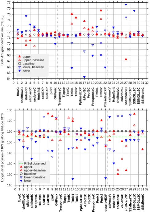
Fig. 9. Sensitivity results for total AIS grounded volume (upper) at LGM and present-day ROSgl position (lower). Note the latter met-ric misfit from observation for the baseline run is∼100 km, which equates to 2–3 grid cells.

to provide both regional tuning of the shelves and palaeo-adjustment. The new SSM component is a physically moti-vated empirical approach that captures both the melt–freeze– melt regimes of the larger shelves and the simpler melt regimes of the peripheral shelves. There are three ensemble parameters to provide some degrees of freedom in the com-ponent. The geometry of the larger shelves is used to adjust the strength of the melt aspect ratio, allowing some regional and temporal evolution.

SSM implementation

We merge the exponential ice shelf front melt law published by Horgan et al. (2011)4with quadratic fits to distance-from-4_{The exponential ice shelf melt law was derived from spatial}

and temporal variations, measured by ICESat laser altimetry data, of the ice surface at the front of the ice shelf. The surface changes were attributed to enhanced basal melt within 60 km of the ice shelf front (Horgan et al., 2011).

0 50 100 150 200 250 300 350 400 450 500 Area (x10

5 km 2)

0 1 2 3 4 5 6 7 8 9 10 11 12 13 14 15 16 17 18 19 20 21 22 23 24 25 26 27 28 29 30 31 32 RIS area upper upper−baseline baseline lower−baseline lower slidsedC _slidhardC flowC sedpresC shelfflowC pinC calvmaxV

GHFmix

P

deselevEXP

TresponseC

TeofC

Hshelfcrit shelfcalvC calvthinC shelfcalv2C SSMfrontTC sedEXP slidEXP HmisfitS 0 50 100 150 200 250 300 350 400 450 500 Area (x10

5 km 2)

0 1 2 3 4 5 6 7 8 9 10 11 12 13 14 15 16 17 18 19 20 21 22 23 24 25 26 27 28 29 30 31 32 FRIS area upper upper−baseline baseline lower−baseline lower slidsedC _slidhardC flowC sedpresC shelfflowC pinC calvmaxV

GHFmix

P

deselevEXP

TresponseC

TeofC

HmisfitS

Fig. 10. Sensitivity results for ROS (upper) and RON-FIL (lower) present-day area.

grounding line transects for the melt rate and the ice shelf thickness measured for AMY (Wen et al., 2007)5and RON (Jenkins and Doake, 1991)6. A flowchart of the implementa-tion is shown in Fig. 2.

The SSM component models three regimes under the larger shelves: a draught-dependent grounding line zone (GLZ) of melt, an accretion zone (ACZ) where freeze-on oc-curs, and a zone of melt at the ice shelf front (SFZ). The smaller shelves only have regions of GLZ and SFZ melt oc-curring. Being on the periphery of the continent, the smaller 5_{The AMY transects were computed from in situ and remote}

sensing datasets; a flow line set of flux gates were defined using the datasets. The mass budgets, basal melting, and freezing rates were derived from the flux gates (Wen et al., 2007).

6_{The RON transects were derived from a glaciological field}

(16)

shelves lack the embayment protection that the larger shelves have. As such, the sub-ice-shelf environment is not suffi-ciently quiescent to allow the mode 1 melt water to freeze-on underneath the ice shelf. For monitoring modelled ice shelf response, the floating ice is divided into five regions (shown in Fig. 3a) pertaining to the four large shelves (AMY, ROS, RON, and FIL), and the ice that is not part of the large shelves (e.g. the smaller shelves of the Amundsen, Weddell, and Bellingshausen seas and the remaining unnamed shelves) is classified as OTHER.

The transitions between the zones were estimated from the AMY and RON transects, shown in Fig. 4a. The raw data for these transects, given in Tables 1 and 2 of the Supplement, were extracted from Wen et al. (2007, Figs. 4 and 6) for AMY and from Jenkins and Doake (1991, Figs. 9 and 10) for RON. The transition from GLZ to ACZ in the larger shelves oc-curs at a shelf thickness of ∼700 m. Similarly the transi-tion from the ACZ to the SFZ occurs at a shelf thickness of approximately 300–400 m. The melt–accretion–melt pat-tern can also be seen, albeit approximately, when compar-ing the 700 m and/or 300 m contour from ALBMAP (Fig. 5) and the satellite-derived melt distribution patterns of AMY (Fricker et al., 2001, Fig. 3), FIL (Joughin and Padman, 2003, Fig. 2), and the modelling study of ROS (Holland et al., 2003, Fig. 10). Sensitivity tests were made adjusting the transition thicknesses within the range of uncertainty in the transects. However, because the melt/accumulation rates before and af-ter the transition zones are very small (Jacobs et al., 1992; Horgan et al., 2011; the dominant melt rates occur at the grounding lines and at the shelf front), there was little im-pact. As such the transition thicknesses are held constant in the SSM component.

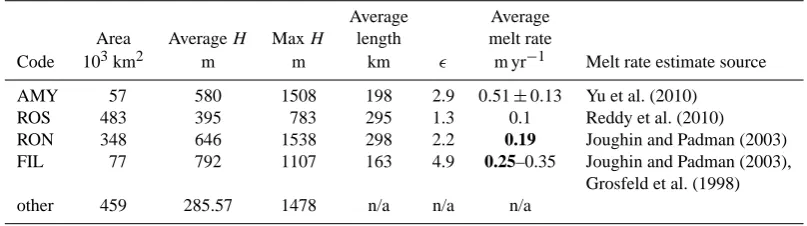
The melt rate in the GLZ is modelled as a function of ice shelf thickness and the aspect ratio of the ice shelf. Plot-ting the melt rate as a function of thickness (Fig. 4b) allows a quadratic best fit to be made (the raw data were pruned so that the quadratic fit is only made with the data that are up-stream of the GLZ-to-ACZ transition thickness threshold; i.e. whereH <700 m the melt rate is set to zero); each transect has a different fit, and thus each ice shelf has a different melt rate thickness function. We hypothesize that, because the larger shelves have distinct cavity geometries that affect the oceanographic processes within them (Fricker et al., 2001; Horgan et al., 2011), the melt function is proportional to the physical dimensions of the ice shelf. We define a thickness-to-length aspect ratio,= [H]/[L], to reflect the cavity di-mensions. Table 4 summarizes the physical characteristics, computed from ALBMAP, used for defining the aspect ratio. The average length is computed as the average minimum dis-tance from each grounding line grid cell to open ocean with-out encountering land or grounded ice. The ice shelf average melt rate magnitudes are taken from Table 3 of the Supple-ment. The stronger melt rates are seen under AMY (thick and short) and FIL (thickest and shortest), which have larger

as-pect ratios than RON (thick and long). ROS (thin and long) has the smallest melt rate.

Using the present-day AMY and RON aspect ratios (AMY, RON) and associated quadratic laws as reference melt functions (_Mg˙

AMY,Mg˙ RON), the GLZ melt rate (Mg) for˙ a shelf of thicknessH(in metres) with aspect ratio (shf) can be computed usingshfas a weighting factor and interpolat-ing between the two reference functions.

˙

Mg_AMY= −7.95×10−06_H2₊₈_.₃₈_×₁₀−03_H₋₂_.₁₉_, ˙

Mg_RON= −5.10×10−06H2+5.92×10−03H−1.62. The ice shelf weighting factor is computed as Wshf= shf−AMY

RON−AMY. (25)

The final GLZ melt rate (m yr−1) is computed from

˙

Mg=fnGLzN _˙

Mg_AMY+WshfMg˙ RON− ˙MgAMY

, (26) where ensemble parameter fnGLzN allows the strength of the computed melt to be adjusted: SSMGLz1C (range 0.5–3) for the larger shelves and SSMGLz2C (range 0.5–2.5) for the OTHER shelves. The aspect ratio for the OTHER shelves is always set to be the maximum of the large shelves, motivated by the fact that they are closer to the CDW so will likely suf-fer stronger melt for a given thickness. As the shelves evolve over time, the aspect ratio will also evolve, reducing or in-creasing the amount of melt proportionally. The calculation of length is computationally costly. As such, it is only per-formed every 20 yr.

The basal accretion (m yr−1) in the ACZ is modelled us-ing a quadratic function that increases from zero at the two transition zones to a maximum near the centre:

˙

Ma= − 1

45 000(H−550)

2₊₀_.₅_. ₍₂₇₎

The maximum accretion is set to be 0.5 m yr−1 for all shelves7. ACZ accumulation, being a product of the GLZ mode 1 melt, should not exceedMg. If this does occur, the˙ totalMa is recomputed to be equal to˙ Mg melt and is re-˙ distributed over the ACZ area. For present day this con-dition only occurs in ROS where, because of the shallow draught, the total GLZ melt is very low. Thus, because of the large area of the ACZ, the redistribution can reduce freeze-on amounts to near 0 m yr−1values (see Fig. 3).

The SFZ melt is modelled in accordance with the expo-nential law presented in Horgan et al. (2011). Within 60 km of the ice shelf front, the melt (m yr−1_{) follows the form}

˙

Ms=(1+SSMfrontTC×(zclim(t )−1)) (28)

×2.0 exp

₋

x 11.9 km

,

7_{From the transects and the RON (Joughin and Padman, 2003,}