A constraint solving approach to model reduction by tropical equilibration

R E S E A R C H

Open Access

A constraint solving approach to model

reduction by tropical equilibration

Sylvain Soliman

, François Fages

and Ovidiu Radulescu

Abstract

Model reduction is a central topic in systems biology and dynamical systems theory, for reducing the complexity of detailed models, finding important parameters, and developing multi-scale models for instance. While singular perturbation theory is a standard mathematical tool to analyze the different time scales of a dynamical system and decompose the system accordingly, tropical methods provide a simple algebraic framework to perform these analyses systematically in polynomial systems. The crux of these methods is in the computation of tropical equilibrations. In this paper we show that constraint-based methods, using reified constraints for expressing the equilibration conditions, make it possible to numerically solve non-linear tropical equilibration problems, out of reach of standard computation methods. We illustrate this approach first with the detailed reduction of a simple

biochemical mechanism, the Michaelis-Menten enzymatic reaction model, and second, with large-scale performance figures obtained on the http://biomodels.net repository.

Keywords: Systems biology, Model reduction, Tropical algebra, Tropical equilibration, Constraint programming

Background

Model reduction is a central topic in systems biology and dynamical systems theory, for reducing the complexity of detailed models, finding important parameters, and developing multi-scale models for instance.

Indeed, for many of the problems in computation and analysis of complex systems, the upper limit on the size of the system that can be studied has been reached. This limit can be very low, namely tens of variables for system identification, symbolic calculation or bifurcation of attractors of large dynamical systems. For instance, the complexity of extant symbolic solvers of polynomial equations is exponential in the number of indeterminates and parameters, that sets a drastic limitation to the size of the models that can be analyzed [1,2]. Some examples of computational difficulties that arise when trying to apply standard tools of algebraic geometry to systems biology models can be found in [3]. Model reduction is a way to bypass these limitations by replacing large scale mod-els with modmod-els containing less parameters and variables, easier to analyse.

*Correspondence: [email protected]

1Inria, Domaine de Voluceau 78150, Rocquencourt, France Full list of author information is available at the end of the article

There are mathematical methods, based on singular perturbations or on the theory of invariant manifolds, allowing reduction of fully parametrized systems with separation of time scales. More precisely, in dissipative systems, fast variables relax rapidly to some low dimen-sional attractive manifold called invariant manifold [4] that carries the slow mode dynamics. A projection of dynamical equations onto this manifold provides the reduced dynamics. Numerical reduction methods, such as computational singular perturbation (CSP, [5]), intrinsic low dimensional manifold (ILDM, [6]) exploit the sep-aration of timescales of various processes and compute approximations of the invariant manifold. Purely struc-tural reduction methods can handle big models possibly with lack of kinetic information [7]. However, the case of biochemical models of intermediate size, with partially known parameters and that ask for symbolic analysis, is more open [8].

While singular perturbation theory is a standard math-ematical tool to analyze the different time scales of a dynamical system and decompose the system accordingly, tropical methods provide a simple algebraic framework to perform these analyses systematically in polynomial systems, and in situations when model parameters are known only by their orders of magnitude. Differential

equations describing kinetics of biochemical reactions are polynomial or become polynomial after decomposition of reaction mechanisms into elementary steps. For these models, quasi-equilibrium or quasi-steady state invari-ant manifolds allowing reductions are given by systems of algebraic equations [3]. A potentially crucial applica-tion of tropical mathematics is to enumerate and describe asymptotic solutions of algebraic systems of equations [9]. In particular, tropical solutions of polynomial equations provide the leading terms of their solutions via curves or in other terms via Newton-Puiseux series [10,11]. At the basis of our method lies the idea that equilibration of fast variables on invariant manifolds implies, at low-est order, equilibration of at least two dominant mono-mials, one positive and the other negative in the right hand side of the differential equations. We have called such a condition, similar to Kapranov’s condition [11] for existence of Newton-Puiseux series with specified low-est order terms, tropical equilibration. The crux of our method lies in the computation of tropical equilibrations that define some reduced truncated systems with fewer parameters to identify, thus pointing to fewer experiments to (in)validate the model [12,13]. Our method copes with uncertain parameters by replacing exact values by orders of magnitude and the reduction is performed symboli-cally in both variables and parameters. With respect to methods based on singular perturbations, this could be less precise at lowest order, but it is more general in implementation.

Solving the tropical equilibration problem boils down to solving a system of equations in the min-plus algebra (also known as the tropical semiring). For solving linear tropical systems there are pseudo-polynomial algorithms, i.e. whose complexity is polynomial in the size of the sys-tem and in the absolute values of its coefficients [14]. In the nonlinear case, the existence of tropical equilibrations, which is equivalent to the problem of the intersection of tropical varieties, was shown to be NP-complete [15]. In this paper we show that constraint-based methods, using reified constraints for expressing the equilibration con-ditions, make it possible to numerically solve non-linear tropical equilibration problems, out of reach of standard computation methods.

We first illustrate this approach with the detailed reduc-tion of a simple biochemical mechanism, the Michaelis-Menten enzymatic reaction model. We detail the general procedure to obtain truncated systems by identifica-tion, through equilibraidentifica-tion, of fast and slow species, and relate the obtained reduced systems to the usual notions of quasi-steady-state and quasi-equilibrium. Then, we demonstrate that the approach is computationally feasi-ble, and scales up properly, by treating in an automatic way all the curated dynamical models of http://biomodels.net repository [16].

Model reduction by tropicalization

We consider networks of biochemical reactions with mass action kinetic laws. The structure of a reaction is defined by a multiset rewriting rule as

n

i=1

αjiAi→ n

k=1

βjkAk

where Ai,i = 1,. . .,n denote the chemical species and αji,βjk are positive integers named stoichiometric coeffi-cients defining which species are consumed and produced by the reactionj, 1≤j≤r, and in which quantities.

The mass action law means that reaction rates are monomial functions of the species concentrationsxi, 1≤ i≤nand read

Rj(x)=kjxαj,

where kj > 0 are kinetic parameters and we use the shorthand notationxαj=_xαj1

1 . . .x αjn

n .

The network dynamics is then described by the follow-ing differential equations

dxi

dt =

r

j=1

kjSijxαj. (1)

where Sij = βji − αji are entries of the stoichiometric matrix.

In what follows, the kinetic parameters do not have to be known precisely, they are given by their orders of magnitude. A convenient way to represent orders is by considering that

kj= ¯kjγj,

whereis a positive parameter much smaller than 1,γjis an integer or, more generally, a rational number, andk¯jhas order unity. An approximate integer order can be obtained from any real positive parameter by

γj=round(log(kj)/log()),

where round stands for the closest integer. Notice that in this representation, small quantities have large orders. Furthermore, the smaller , the better the separation between quantities of different orders, indeed lim→0k_ki_j = ∞, ifγi< γj.

We also define orders for species concentrations, using a vector of ordersa=(a1,. . .,an), such thatx= ¯xa. We suppose that various(a1,. . .,an)are integers or rational numbers with a common denominator. In our method we will calculate the concentration orders as solutions of the tropical equilibration problem (see below).

First, let us replace Eqs. (1) by their equivalent rescaled versions

dx¯i

dt =

r

j=1

μj−ai_k

where

μj=γj+<a,αj>, (3) and<,>stands for the vector dot product.

The r.h.s. of each equation in (2) is a sum of multi-variate monomials in the concentrations. The ordersμj indicate how large are these monomials, in absolute value. For sufficiently small, monomials of different orders are well separated. For instance a monomial of smallest order

μj < μj dominates the other monomials kj|Sij|xαj kj|Sij|xαj. One could see all these monomials as “forces” acting on the chemical species. At steady state, the resul-tant of all these forces should be naught. A consequence of this is that the orders of dominant positive and neg-ative forces should be equal. This is exactly our notion oftropical equilibrationthat we introduced in [13]. More precisely, we say the system (2) istropically equilibratediff

min(μj,Sij<0)=min(μj,Sij >0), for all i=1,. . .,n (4)

The tropical equilibration problem consists in solving the system (4) for ordersai, 1≤i≤n.

Another way to understand the condition (4) is via Newton-Puiseux series. Suppose we want to solve the polynomial equation

P(x,)=

j

bjγjxαj =0, (5)

whereαjare positive integers,γjare rational powers, and bjare real coefficients. It is well known [10] that solutions of this equation can be expressed as Newton-Puiseux series, i.e. have the form

x()=c1

a₁ q +_c

2

a₂ q +. . ._,

where ci are complex coefficients, a1 < a2 < . . . are integers, q is a positive integer. By substituting x() = c1

a₁ q (₁+_x

1())(wherex1()collects terms with positive orders in) in (5) we get

P(x,)=

j

bjcα1jγj+a1αj/q+r1()=0,

wherer1()collects higher order terms. Necessary condi-tions forP(x,)=0 read at lowest order

j,γj+a1αj/q=m

bjcα1j=0 (6)

m=min

j (γj+a1αj/q) (7)

In order to satisfy (6), the minimum in (7) should be attained at least twice. Furthermore, if one looks for real solutionsci ∈R, then from (6) it follows that at least two bj corresponding to the minimum (7) should have oppo-site signs. This means that the lowest ordera1/q in the

Newton-Puiseux series solution has to satisfy a tropical equilibration problem.

We must emphasize that the tropical equilibration con-dition is weaker than the steady state concon-dition, and makes sense also away from a steady state. In systems with slow/fast variables, the fast variables are equilibrated by compensation of dominant forces whose orders result from the tropical condition (4). As a consequence, the fast variables can be expressed as functions of the slow vari-ables. However, both fast and slow variables can slowly evolve under the influence of weaker, higher order forces. This picture is valid as long as the relative dominance relations between various monomial terms in Eqs.(2) are preserved. This is true if the rescaled concentrations x¯i stay between bounds, whereasis allowed to tend to zero. To summarize, the tropical equilibration is a neces-sary condition for the elimination of fast variables and model reduction. As we showed in [13], in order to become sufficient this condition should be combined with a boundedness condition, called permanency:

Definition 0.1.The system (1) is permanent, if there are two constants C− > 0and C+ > 0, a set of renor-malization exponents ai, and a function T0of the initial conditions, such that after renormalization we have

C−<x¯i(t) <C+, for all t>T0(x(0))and for every i.

A simple example, the Michaelis-Menten reduction The Michaelis-Menten enzymatic reaction network con-sists of three reactions:

S+E k1 k−1

ES→k2 P+E,

where S,ES,E,P represent the substrate, the enzyme-substrate complex, the enzyme and the product, respec-tively.

The corresponding system of polynomial differential equations reads:

x₁= −k1x1x3+k−1x2 x₂=k1x1x3−(k−1+k2)x2 x₃= −k1x1x3+(k−1+k2)x2 x₄=k2x2

(8)

wherex1=[S],x2=[ES],x3=[E],x4=[P].

It can be easily checked that the system has two alge-braic invariants:(x2+x3)=0, which implies

x2+x3=e0, (9)

where e0 is a positive constant (the total amount of enzyme), and

wheres0is a positive constant (the total amount of sub-strate and product). These conservation laws can be used to reduce the model by elimination ofx4(by (10)) andx3 (by (9)). It follows:

x₁= −k1x1(e0−x2)+k−1x2 x₂=k1x1(e0−x2)−(k−1+k2)x2

(11)

The constraintx2≤e0resulting from the elimination is also to consider, but we will see that all equilibrations of the above equations already imply it.

Tropical equilibration equations

By rescaling variables and parameters, we getxi = ¯xiai, 1≤i≤2,k1= ¯k1γ1,k−1= ¯k−1γ−1,e0= ¯e0γe.

The tropical equilibration equations for the reduced system read:

γ1+γe+a1=min(γ1+a1,γ−1)+a2 (12)

γ1+γe+a1=min(γ1+a1, min(γ−1,γ2))+a2 (13) The set of integer (or rational) orders endowed with the ⊕ = min and⊗ = + operations is a semi-field, called min-plus algebra or tropical field [17]. In this semi-field, −∞ plays the role of 0 and 0 plays the role of 1. The multiplicative inverse ofais denoted−a. Our tropical equilibration problem means solving a set of polynomial equations in this semi-field. Using these notations and properties of semi-field operation, the tropical equations become:

γ1⊗γe⊗a1⊗(−a2)=(γ1⊗a1)⊕γ−1 (14)

γ1⊗γe⊗a1⊗(−a2)=(γ1⊗a1)⊕γ−1⊕γ2 (15)

Classical Michaelis-Menten reduction

The classical derivation of the Michaelis-Menten reduc-tion is based on the behaviour of the variable x2for the complex concentration. Using (8) it follows that:

x₄=Vmx2/e0

whereVm=k2e0is the maximum value of the production ratex₄, sincex2≤e0.

The variablex2satisfies equilibration relations and can be expressed as a function of a slow variable (either the substrate x1 when x2 is small, or the sum x1 + x2 in general) in two situations: stationarity and quasi-equilibrium.

The quasi-stationarity corresponds to settingx₂to zero and is justified by the smallness of x2 that can be con-sidered a fast species (radical). More precisely one has k1x1(e0 − x2) − (k−1 + k2)x2 = 0, leading to x2 = x1e0/(Km+x1), whereKm=(k−1+k2)/k1, i.e.

x₄=Vmx1/(Km+x1) (16)

The quasi-equilibrium corresponds to setting k1x1

(e0 − x2) − k−1x2 = 0, meaning zero net flux of the first reaction in the mechanism. This leads to x2 = x1e0/((k−1/k1)+x1), i.e.

x₄=Vmx1/((k−1/k1)+x1) (17)

This is justified by having a very fast transformations in the direct and reverse sense by the first reaction, much faster than the transformations by the second reaction. In this case bothx1andx2are fast, but their sumx1+x2is slow.

We show next, in Section “Tropical equilibrations and model reductions”, that analysis of tropical equations pro-vide the conditions for the asymptotic validity of quasi-stationarity and quasi-equilibrium approximations and also the exhaustive list of asymptotic regimes.

Geometrical interpretation

It was discussed in [13] that there is a bijection between the set of solutions of each tropical equation and parts of the tropical curves of the polynomials defining the ordi-nary differential equations. A tropical curve is defined as the locus of species concentration values(x,y) where at least two monomials of the considered polynomial are equal and larger than all the others. In logarithmic scale, this locus is made of lines, half-lines, or line seg-ments [13,18]. There is one tropical curve for each differ-ential equation. For instance, the tropical curve defined by the polynomial−k1e0x1+k1x1x2+k−1x2is made of three half-lines with a common origin depicted in Figure 1, namely

log(x2)=log(e0), log(x1) >log(k−1/k1) (18)

log(x1)=log(k−1/k1), log(x2) >log(e0) (19)

log(x2)=log(x1)+log(e0k1/k−1), log(x1) <log(k−1/k1) (20)

The solutions of the tropical equation (14) form two branches, corresponding to the two situations(γ1⊗a1)⊕

γ−1=(γ1⊗a1)and(γ1⊗a1)⊕γ−1=γ−1, respectively. These are two half-lines in the plane of concentration orders:

a2=γe, γ1+a1< γ−1 (21)

Figure 1Tropical curves in the planes of concentrations and orders for the two variables Michaelis-Menten model.Tropical curves are defined as the locus of points where two monomials of a polynomial describing a differential equation are equal. The tropical curves for each differential equations are indicated by colors, blue for the first equation and red for the second equation. The vertical half-line of each of the tripods does not carry tropical equilibrations because it corresponds to equality of two monomials of the same sign. The horizontal and the oblique half-lines of the tripods carry tropical equilibrations. We have represented the two situations whenk₋1>k2and whenk−1<k2. All the tropical equilibrations are double (both variables are equilibrated) in the first case, and can be simple (only one variable is equilibrated) in the latter.

The two branches of solutions can be also related to parts of the tropical curves corresponding to the equili-bration of monomials of different signs. More precisely (21) corresponds to (18), and (22) corresponds to (20). The branch (19) of the tropical curve corresponds to the equal-ity of two positive monomials and has no correspondence in the set of tropical equilibrations.

Similarly to computing steady states as intersections of null-clines, we are considering multiple tropical equilibra-tions as intersecequilibra-tions of tropical curves.

We therefore consider the second tropical equation (15), in two situationsγ₋1⊕γ2 = γ−1andγ−1⊕γ2 = γ2. In the first case the tropical equation (15) is equivalent to the tropical equation (14) (also, the tropical curves coincide). Therefore, the two solutions (21) and (22) equilibrate both equations. In the second case, the solutions of the trop-ical equation (15) form two branches, corresponding to

(γ1⊗a1)⊕γ2=γ1⊗a1and(γ1⊗a1)⊕γ2=γ2, respec-tively. They correspond to two half-lines in the plane of orders (a1,a2), namely a2 = γe, a1 < γ2− γ1 and a2=a1+γ1+γe−γ2, a1> γ2−γ1. A simple graph-ical inspection of the relative positions of these half-lines with respect to the half-lines carrying solutions of the first tropical equation shows that there are four branches of tropical equilibrations:

a2=γe, a1< γ2−γ1 (23)

a2=γe, γ2−γ1<a1< γ2−γ1 (24)

a2=a1+γ1+γe−γ2, a1> γ2−γ1 (25)

a2=a1+γ1+γe−γ−1, a1> γ−1−γ1 (26)

The branch (23) equilibrates the two variables. The branch (25) equilibrates only the second variable, whereas the branches (24), (26) equilibrate only the first variable.

Tropical equilibrations and conservation laws

considering equilibration of dominant terms, leads to the tropical problem:

γ1⊗a1⊗a3=γ−1⊗a2 (27)

γ1⊗a1⊗a3=(γ−1⊗a2)⊕(γ2⊗a2) (28)

a2⊕a3=γe (29)

This tropical problem is different from (14), (15) and leads to different solutions in general. Firstly, let us notice that elimination is not possible in semi-fields, because there is no additive inverse in general. Hence, (27), (28) (29) can not be reduced to an equivalent system of two tropical equations. Secondly, dominant monomial equilibration in the reduced model does not always cor-respond to monomial equilibrations in the unreduced model. A typical example is the monomial x1x3 that becomes the differencex1e0−x1x2in the reduced model. The two monomials can equilibrate each other in the reduced model, but the same quantity is an unique, un-equilibrated monomial in the full model.

There are six branches of tropical solutions of the sys-tem (27), (28), (29). Two branches are obtained when

γ−1 ⊗ a2 = γ−1. In this case the two tropical equations (27), (28) are identical. Depending ona2⊕a3= a2, ora2⊕a3=a3we get:

a2=γe, a1< γ−1−γ1 (30)

a2=a1+γ1+γe−γ−1, a1> γ−1−γ1 (31)

These branches correspond to equilibrations of all the variables.

When γ₋1 ⊗a2 = γ2 the two tropical Eqs. 27, (28) are incompatible. Depending on a2⊕a3 = a2, ora2⊕ a3=a3and further choosing only one of the two tropical Eqs. 27, (28) we get the following branches:

a2=γe, a1< γ−1−γ1 (32)

a2=γe, a1< γ2−γ1 (33)

a2=a1+γ1+γe−γ−1, a1> γ−1−γ1, (34)

a2=a1+γ1+γe−γ2, a1> γ2−γ1 (35)

In the branches (32), (34), the variablesx2,x3are not equilibrated, whereas in the branches (33), (35), the vari-ablex1is not equilibrated.

Comparison of Eqs. (30)-(35) and Eqs. (21)-(26) proves that the tropical equations of the unreduced model have

the same set of solutions as the reduced model. However, the branch of solutions (33) equilibrates all the variables in the reduced model and does not equilibrate the vari-ablex1 in the reduced model. The reason is exactly the one given above: the monomialx1x3is dominant and un-equilibrated in the unreduced model, becomesx1e0−x1x2 with equilibrated monomials in the reduced model.

Tropical equilibrations and model reductions

Tropical equilibrations can be used for model reduction. The reduction starts by tropical truncation. We call trop-ically truncated model the model obtained by elimination of all dominated monomials from the r.h.s. of the ordinary differential equations. The next step is ordering the vari-ables according to the values of the exponentsμi−ai. This allows to determine which variables are slow and fast.

An additional construction is needed in the case when the tropically truncated system of fast variables has con-servation laws that are not conserved by the un-truncated system. The conservation laws define species pools that are supplementary slow variables. The pools follow differ-ential equations involving previously dominated monomi-als.

For instance, in the two variables Michaelis-Menten model, we found essentially two types of reduced models, corresponding to equilibrium and quasi-stationarity approximations [19].

The branch (21) of tropical solutions leads to the follow-ing truncated system:

x₁= −k1x1e0+k−1x2 x₂=k1x1e0−k−1x2

(36)

This truncated system has conserved quantityz=x1+ x2. The variable z is not conserved by the full model described by (11). Indeed, addition of Eqs. (11) leads to z = −k−1x2. As the variable x2 can be eliminated from −k1x1e0+ k−1x2 = 0 andx1 +x2 = z we have the reduced dynamicsz = −kzz, wherekz = k−1/(1+ k₋1/(k1e0)). For small, we can consider thatkz ∼ γz, with γz = γ−1−min(0,γ−1−γ1 −γe). Because μ1− a1 = γ1 +γe, μ2 −a2 = γ1+ γe +a1− a2 = γ−1 the relation kz > μ1 − a1, kz > μ2 − a2 are always satisfied guaranteeing that z is slower than x1, x2. The form (36) of the truncated equations and the conservation ofx1+x2by the fast dynamics shows that this case cor-responds to quasi-equilibrium of the first reaction in the Michaelis-Menten model, as described in Section “Classi-cal Michaelis-Menten reduction”, equation 17.

The branches (23) and (24) lead to quasi-equilibrium with the following truncated system:

x₁= −k1x1(e0−x2) x₂=k1x1(e0−x2)

These cases correspond to saturation of the enzyme (x2 has the same order ase0). A slow variablez=x1+x2has to be introduced as before, but the reduced dynamics is z= −k₋1x2= −k−1e0.

The branch (25) leads to quasi-stationarity of the enzyme/substrate complex. In this case we have the trop-ical truncated system:

x₁= −k1x1e0 x₂=k1x1e0−k2x2

(38)

The variable x1 is not equilibrated, which still allows for model reduction because this variable is slow. The fast variable x2 is equilibrated, and the equilibration equation corresponds to the classical notion of quasi-stationary approximation, as described in Section “Clas-sical Michaelis-Menten reduction”, equation 16. In this case,μ1−a1=γ1+γe,μ2−a2=γ1+γe+a1−a2=γ2. The condition thatx1is slower thanx2readsμ1−a1 >

μ2−a2and we get the additional conditionγ1+γe> γ2, which is a low enzyme concentration condition.

The branch (26) leads to quasi-stationarity of the sub-strate with the following truncated system:

x₁= −k1x1e0+k−1x2, x₂= −k2x2

(39)

The variablex2is not equilibrated, which is allowed only if this variable is slower thanx1. In this case,μ1−a1 =

γ1+γe,μ2−a2=γ2. The condition thatx2is slower than x1readsμ1−a1< μ2−a2and leads to the additional con-ditionγ1+γe< γ2, which is a high enzyme concentration condition.

Finally, the branch (24) leads to the truncated system:

x₁= −k1x1(e0−x2) x₂= −k2x2

(40)

The variablex1is equilibrated, but it can not satisfy per-manency. Indeed, at fixedx2this variable will converge to zero. Therefore, this tropical equilibration does not lead to a reduced model.

Tropical equilibration as a constraint satisfaction problem

As explained in Section “Model reduction by tropical-ization”, given a biochemical reaction system with its Mass-Action kinetics, and a small, the problem of trop-ical equilibration is to look for a rescaling of the variables such that the dominating positive and negative term in each ODEequilibrateas per Eqs. (4), i.e., are of the same degree in.

Section “A simple example, the Michaelis-Menten reduction” showed that it is possible to iteratively reduce the equilibration problem to a linear system of equations for each possible pair of positive and negative dominating

monomial. It is actually possible to consider fewer pairs by restricting that search to the pairs denoting edges of the Newton polygon [13]. Nevertheless, the number of linear systems to consider remains exponential in the number of species, and may lead to redhibitory computational costs, especially when handling biochemical systems with hub molecules, i.e., molecules involved in a high num-ber of reactions (e.g., E2F, p53, cMyc in cell-cycle control or NFκB in signalling), which corresponds to a Newton polygon with many vertices.

In order to tackle that complexity, we propose a numer-ical approach based on Constraint Programming, that encodes the equilibration problem as a Constraint Satis-faction Problem (CSP) [20-22] and uses reified constraints to prune the search space. Constraint Programming is a paradigm that has showed great success at solving combi-natorial decision or optimization problems, in particular for real-world instances of NP-hard problems, e.g., in the field of production planning and scheduling. It is there-fore an interesting way to approach the combinatorial explosion described above.

In presence of invariants (conservation laws) in the orig-inal system, Section “Conservation law constraints” has shown that some constraints related to rescaling need be added. We have shown in [23] that finding these conserva-tion laws can be efficiently solved by constraint methods. Here we will thus assume that the conservation laws are given in input. In our prototype implementation, both the computation of conservation laws and the following equilibration are performed for a given system.

Reified constraints

Key to the modeling of tropical equilibration problems as CSP are reified constraints. Reified constraints are special constraints that link in a bidirectional way the value of a boolean variable to the satisfaction of another constraint. They allow for powerful cuts in the search space by prop-agating the truth value of some constraints of the problem to the truth value of the Boolean variable, and vice versa.

For instance, the reified constraint

B#<==>X#=Y

states that the Boolean variableBis true (i.e. equal to 1) if and only if the constraintsX = Y is satisfied. That con-straint posts the concon-straintX= Y(resp.X =Y) as soon asB gets value 1 (resp. 0), and vice versa, sets B = 1 (resp.B=0) as soon asX=Y(resp.X=Yi.e. when the domains ofXandYbecome disjoint).

many things on the domains ofA, BandCbefore even-tually tryingA = Bor A = C. For instance it is safe to add thatA ≤ BandA ≤ C, but also if you have, from other equations, thatB ≥minBandC ≥ minC then you can add the fact thatA ≥ min(minB,minC). If later you obtain that actuallyA = Bthen you can enforceC ≥ B, etc. Section “Minimum constraints” shows in more detail how reified constraint do precisely this kind of conditional addition of cuts and can therefore be used to handle mini-mum constraints while postponing enumerative search as much as possible.

Variables and domains

For practical reasons, mainly the lack of an efficient solver over rationals with reified constraints, we use a finite domain solver and therefore only look for inte-ger solutions (whereas solutions are rational). In practice this did not seem to change much the nature of results, see Figure 2. Extensions of the approach to cope with half-integer solutions or with rational solutions with a common, small denominator are straightforward.

For each original equationdxi/dt, 1 ≤ i ≤ nis intro-duced a variableai ∈Zthat is used to rescale the system by posingxi = aix¯i. These are the variables of our CSP. Note that they require a solver handlingZlike for instance SWI-Prolog [24,25] with the clpfd library by Markus Triska, which we used for our implementation.

Tropical equilibration constraints

For each differential equation that should be equilibrated is a list of positive monomialsM_i+, and a list of negative monomialsM_i−. The degrees inof all these monomials are integer linear expressions in theai. Now, to obtain an equilibration one should enforce for eachithat the min-imum degree inM+_i is equal to the minimum degree in M−_i . This corresponds to the Eqs. 4. We will see how they can be implemented with reified constraints, but for now,

let us assume a constraint min(L, M)| that enforces that the variable M ofZis the minimum value of a list L of lin-ear expressions over variables ofZ. We have in our CSP, for each 1 ≤ i ≤ n, min(PositiveMonomialDegrees, M) and min(NegativeMonomialDegrees, M).

Conservation law constraints

The second kind of constraint comes from conservation laws. Each conservation law is an equality between a linear combination of thexiand a constantci. By rescal-ing, we obtain a sum of rescaled monomials equal to

log(ci)/log()_c¯

i. We want this equality to hold whengoes to zero, which implies that the minimal degree inin the left hand side is equal to (the round of ) the degree of the right hand side. Since once again the degrees on the left are linear combinations of our variables ai, this is again a constraint of the form: min(ConservationLawDegrees, K) where K is equal to round(log(ci)/log()). This corre-sponds to the tropical equation (29).

Minimum constraints

Furthermore, if the system under study is not at steady state, the minimum degree should not be reached only once, which would lead to a constant value for the corre-sponding variable when goes to zero, but at least twice. This is the case for the example treated in [12]. The con-straint we need is therefore slightly more general than min/2: we need the constraint min(L, M, N) which is true if M is smaller than each element of L and equal to N elements of that list. Note that using CLP notation, we have:

min(M, L) :− C#>=1, min(M, L, C).

In order to enforce that the minimum is reached at least a required number of times, one obvious solution is to try all pairs of positive and negative monomials and

count the successful pairs [26]. However, this is not nec-essary, the min(L, M, N) constraint directly expresses the cardinality constraint on the minimums and can be imple-mented usingreified constraintsto propagate information between L, M and N in all directions, without enumera-tion. Using SWI-Prolog notations, the implementation of min/3 by reified constraints is as follows:

min([ ] ,,0).

min([ HT] , M, C):−M#=<H, B#<==> M#=H, C#=B+CC, min(T, M, CC).

The translation of this predicate into words is roughly as follows, first ignoring the counts: M is smaller than a list with head H and tail T, if it is smaller than the tail T and it is smaller than the head, i.e., M≤H. Now, we also impose that the value M is reached C times as follows: it is reached CC times in the tail and C=B+CC where B is a variable equal to 1 iff M is equal to the head and 0 otherwise. Note that this latest statement is enforced through a reified con-straint, it will therefore not lead to immediate branching but to the propagation of as much information as possi-ble (e.g., if some values in the list are already known to be strictly greater than others, the corresponding boolean for each of them will be set to 0, and thus the sum will by necessity enforce some other values to be equal to the required minimum).

This concise and portable implementation will probably improve when the minimum and minnglobal constraints are available (see [27] for a reference). However it already proves very efficient as demonstrated in the next section.

When C is equal to one, we can fall back to using the built-in min construct in a constraint (e.g., M #= min(L1, min(L2, L3))). Some preliminary benchmarking showed that the reified version is more efficient if the length of the list is greater than 3 or 4.

Enumeration strategy

Constraints over finite domains come with domain fil-tering algorithms which dynamically prune the domain of variables when the domain of other variables change in a constraint. However this strategy is not complete and must be combined with a search procedure for vir-tually enumerating all possible values of the variables. For this application we obtained good performances with dichotomic search by bissecting the domain of the vari-ables (bisect option in SWI-Prolog) without any particular heuristics for choosing the variables.

Note that since this approach is numerical, contrary to solvingsymbolicallyan exponential but finite number of linear systems as done in Section “A simple example, the Michaelis-Menten reduction” and in [13], there can be an infinite number of solutions. This situation denotes an

under-constrained linear system and remains to be inter-preted biologically. In practice bounds are put on variables in order to force finiteness. This is not a restriction in practice since biochemical species’ concentrations usually do not vary by more than a hundred of magnitude orders. Furthermore, in order to speed-up the computation of all solutions in such large domains, we used an iterative domain expansion strategy: the problem is first tried with a domain of [−2, 2] for all variables , i.e., equilibrations are searched by rescaling in the 10−2, 102interval. If that fails, the domain is doubled and the problem tried again until a limit of 10−128, 10128.

Computation results on Biomodels.net

To benchmark our approach, we applied it systematically to all the dynamical models of the curated part of the http://biomodels.net repository [16] of biological systems, withset arbitrarily to 0.1.

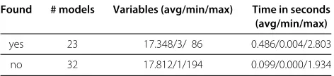
We used release r24 from 2012-12-12 which includes 436 curated models. Among them, only 55 models have non-trivial purely polynomial kinetics (ignoringeventsif any). Our computational results on those are summarized in Table 1, where the first column indicates whether a complete equilibration was found, and the times are in seconds.

The domain expansion strategy coupled with dicho-tomic search by domain bisections allowed us to gain two orders of magnitude of computation time on the biggest models.

Only one of the models (number 002) used values far from 0 in the equilibration (up to40) and has no complete equilibration if the domain is restricted to [−32, 32]. This is because the model is written with units such that the ini-tial concentrations are of the order 10−21_{, translating the} search accordingly. We thus do not believe that enlarging the domains even more would lead to more equilibra-tions. Nevertheless, choosing a smaller might increase the number of equilibrations.

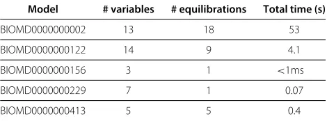
18 of the 23 models for which there is a complete equi-libration are actually under-constrained and appear to have an infinity of such solutions (typically linear rela-tions between variables). For the 5 remaining ones, we computed all complete equilibrations as shown in Table 2.

Table 1 Number of models of the BioModels repository, with a polynomial kinetics, for which tropical

equilibrations were found or not, with corresponding size of the model and computation time

Found # models Variables (avg/min/max) Time in seconds (avg/min/max)

yes 23 17.348/3/ 86 0.486/0.004/2.803

Table 2 Number of equilibrations and computation time for the models of the BioModels database with finitely many numerical solutions

Model # variables # equilibrations Total time (s)

BIOMD0000000002 13 18 53

BIOMD0000000122 14 9 4.1

BIOMD0000000156 3 1 <1ms

BIOMD0000000229 7 1 0.07

BIOMD0000000413 5 5 0.4

Conclusions

In this paper we have shown that constraint-based meth-ods can be efficiently used to numerically solve tropical equilibration problems in biological models of real-size in the BioModels.net repository. These calulations are important for model reduction and for determining the unknown orders of the variables. Once the orders of the variables are known, the rapid variables can be identified and the system reduced to a simpler one. This trunca-tion, described in Section “Tropical equilibrations and model reductions” coupled with the proposed constraint-based method for finding equilibrations therefore pro-vides an automatic way to reduce models and to identify fast/slow variables. We have started the application of such technique on non-trivial models provided by biolo-gists and modellers and hope to be able to improve both the understanding, through that identification of fast/slow variables, and the analysis, through the size reduction, of those models.

Even with the progress of high-throughput technolo-gies, having more focused models, with fewer species and parameters to measure, will definitely permit an improve-ment in the quality and speed of developimprove-ment of the models. Furthermore, the structural methods for com-paring models in model repositories, such as [7], can be refined by filtering the structural reduction relationships according to the kinetics of the reactions and the tropical reasoning on the magnitude orders.

In many cases, it makes sense biologically to only look for partial equilibrations. Strategies to decide when such decision has to be made remain unclear. Nevertheless the framework of partial constraint satisfaction and more specifically Max-CSP [28] would allow us to easily handle the maximization of the number of equilibrated variables. One of the limits of this approach, is that it is not particularly well suited to equilibration problems with an infinite number of solutions. As discussed at the end of previous section, in such situations symbolic solu-tions would be more appropriate. Nevertheless, even the approximate detection of such a case by the very high number of (bounded) numerical solutions was shown to be not very costly in practice.

Competing interests

The authors declare that they have no competing interests.

Authors’ contributions

FF and OR designed the study. SS devised the algorithm and conducted the experiments. All authors equally contributed to the writing of the manuscript. All authors read and approved the final manuscript.

Acknowledgements

This work has been supported by the French ANR BioTempo, CNRS Peps ModRedBio, EPIGENMED Excellence Laboratory and OSEO Biointelligence projects.

Author details

1_{Inria, Domaine de Voluceau 78150, Rocquencourt, France.}2_{University of}

Montpellier 2, Place Eugene Bataillon, 34095 Montpellier, France.

Received: 4 April 2014 Accepted: 4 November 2014

References

1. Grigoriev D, Vorobjov N:Solving systems of polynomial inequalities in subexponential time.J Symbolic Computat1988,5:37–64.

2. Grigoriev D:Complexity of quantifier elimination in the theory of ordinary differential equations.Lect Notes Comput Sci1989,18:11–25. 3. Pantea C, Gupta A, Rawlings JB, Craciun G:The QSSA in chemical

kinetics: as taught and as practiced.InDiscrete and Topological Models in Molecular Biology. Berlin: Springer; 2014:419–442.

4. Gorban A, Karlin I:Invariant manifolds for physical and chemical kinetics.Lect Notes Phys2005,660:1–491.

5. Lam S, Goussis D:The CSP method for simplifying kinetics.Int J Chem Kinet1994,26(4):461–486.

6. Maas U, Pope SB:Simplifying chemical kinetics: intrinsic

low-dimensional manifolds in composition space.Combustion Flame

1992,88(3):239–264.

7. Gay S, Soliman S, Fages F:A graphical method for reducing and relating models in systems biology.Bioinformatics2010,

26(18):i575–i581. [Special issue ECCB’10].

8. Radulescu O, Gorban AN, Zinovyev A, Noel V:Reduction of dynamical biochemical reactions networks in computational biology. Front Genet2012,3:131. [http://www.frontiersin.org/bioinformatics_ and_computational_biology/10.3389/fgene.2012.00131/abstract] 9. Sturmfels B:Solving systems of polynomial equations, Volume 97. American

Mathematical Soc: Providence; 2002.

10. Walker RJ:Algebraic curves. New York: Springer; 1978.

11. Einsiedler M, Kapranov M, Lind D:Non-archimedean amoebas and tropical varieties.J für die reine und angewandte Mathematik (Crelles J)

2006,2006(601):139–157.

12. Noel V, Grigoriev D, Vakulenko S, Radulescu O:Tropical geometries and dynamics of biochemical networks application to hybrid cell cycle models.Electron Notes Theor Comput Sci2012,284:75–91.

13. Noel V, Grigoriev D, Vakulenko S, Radulescu O:Tropicalization and tropical equilibration of chemical reactions.InTropical and Idempotent Mathematics and Applications, Volume 616 of Contemporary Mathematics. Edited by Litvinov G, Sergeev S: American Mathematical Society; 2014:261–277.

14. Grigoriev D:Complexity of solving tropical linear systems. Comput Complexity2013,22:71–88.

15. Theobald T:On the frontiers of polynomial computations in tropical geometry.J Symbolic Comput2006,41(12):1360–1375.

16. le Novère N, Bornstein B, Broicher A, Courtot M, Donizelli M, Dharuri H, Li L, Sauro H, Schilstra M, Shapiro B, Snoep JL, Hucka M:BioModels Database: a free, centralized database of curated, published, quantitative kinetic models of biochemical and cellular systems. Nucleic Acid Res2006,1(34):D689–D691.

17. Cohen G, Gaubert S, Quadrat J:Max-plus algebra and system theory: where we are and where to go now.Ann Rev Control1999,23:207–219. 18. Viro O:From the sixteenth Hilbert problem to tropical geometry.

19. Gorban AN, Radulescu O, Zinovyev AY:Asymptotology of chemical reaction networks.Chem Eng Sci2010,65(7):2310–2324. [International Symposium on Mathematics in Chemical Kinetics and Engineering]. 20. Mackworth AK:Consistency in networks of relations.Artif Intell1977,

8:99–118.

21. Meseguer P:Constraint satisfaction problems: an overview.A.I. Commun1989,2:3–17.

22. Kumar V:Algorithms for constraint- satisfaction problems: a survey. A.I. Mag1992,13:32–44.

23. Soliman S:Invariants and other structural properties of biochemical models as a constraint satisfaction problem.Algorithms Mol Biol2012,

7(15):15.

24. Wielemaker J, Schrijvers T, Triska M, Lager T:SWI-Prolog.Theory Prac Logic Program2012,12(1-2):67–96.

25. Wielemaker J:SWI-Prolog 6.3.15 Reference Manual; 1990. [http://www.swi-prolog.org/pldoc/refman/]

26. Radulescu O, Gorban A, Zinovyev A, Noel V:Reduction of dynamical biochemical reaction networks in computational biology. Front Bioinformatics Comput Biol2012,3:131.

27. Beldiceanu N, Carlsson M, Demassey S, Petit T:Global constraints catalog.Tech. Rep. T2005-6, Swedish Institute of Computer Science 2005. 28. Freuder EC, Wallace RJ:Partial constraint satisfaction.Artif Intell1992,

58:21–70.

doi:10.1186/s13015-014-0024-2

Cite this article as:Solimanet al.:A constraint solving approach to model reduction by tropical equilibration.Algorithms for Molecular Biology

20149:24.

Submit your next manuscript to BioMed Central and take full advantage of:

• Convenient online submission

• Thorough peer review

• No space constraints or color figure charges

• Immediate publication on acceptance

• Inclusion in PubMed, CAS, Scopus and Google Scholar

• Research which is freely available for redistribution