RESEARCH
Crime topic modeling
Da Kuang
1, P. Jeffrey Brantingham
2*and Andrea L. Bertozzi
1Abstract
The classification of crime into discrete categories entails a massive loss of information. Crimes emerge out of a complex mix of behaviors and situations, yet most of these details cannot be captured by singular crime type labels. This information loss impacts our ability to not only understand the causes of crime, but also how to develop optimal crime prevention strategies. We apply machine learning methods to short narrative text descriptions accompany-ing crime records with the goal of discoveraccompany-ing ecologically more meanaccompany-ingful latent crime classes. We term these latent classes ‘crime topics’ in reference to text-based topic modeling methods that produce them. We use topic distributions to measure clustering among formally recognized crime types. Crime topics replicate broad distinctions between violent and property crime, but also reveal nuances linked to target characteristics, situational conditions and the tools and methods of attack. Formal crime types are not discrete in topic space. Rather, crime types are dis-tributed across a range of crime topics. Similarly, individual crime topics are disdis-tributed across a range of formal crime types. Key ecological groups include identity theft, shoplifting, burglary and theft, car crimes and vandalism, criminal threats and confidence crimes, and violent crimes. Though not a replacement for formal legal crime classifications, crime topics provide a unique window into the heterogeneous causal processes underlying crime.
Keywords: Machine learning, Non-negative matrix factorization, Text mining, Crime
© The Author(s) 2017. This article is distributed under the terms of the Creative Commons Attribution 4.0 International License (http://creativecommons.org/licenses/by/4.0/), which permits unrestricted use, distribution, and reproduction in any medium, provided you give appropriate credit to the original author(s) and the source, provide a link to the Creative Commons license, and indicate if changes were made.
Background
Upon close inspection, the proximate causes of crime can be traced to subtle interactions between situational con-ditions, behavioral routines, and the boundedly-rational decisions of offenders and victims (Brantingham and Brantingham 1993). Consider two crimes. In one event, an adult male enters a convenience store alone in the middle of the night. Brandishing a firearm, he compels the store attendant to hand over liquor and all the cash in the register (Wright and Decker 1997:89). This event may be contrasted with a second involving female sex worker who lures a john into a secluded location and takes his money at knife point, literally catching him with his pants down (Wright and Decker 1997:68). In spite of the fine-grained differences between these events, both end up classified as armed robberies. As a matter of law, the classification makes perfect sense. The law favors a bright line to facilitate classification of behavior into that which is criminal and that which is not (Casey and Niblett 2015;
Glaeser and Shleifer 2002). The loss of information that comes with condensing complex events into singular cat-egories, however, may hamper our ability to understand the immediate causes of crime and what might be done to prevent them, though the quantitative tractability gained may certainly offset some of the costs.
The present paper explores methods for crime clas-sification based directly on textual descriptions of crime events. Specifically, we borrow methods from text mining and machine learning to examine whether crime events can be classified using text-based latent topic modeling (e.g., Blei 2012). Our approach hinges on the idea that the mixtures of behavioral and situational conditions under-lying crime events that are captured at least partially in textual descriptions of those events. These text descrip-tions of the event itself might be from the perspective of the offender, police or third party. We focus on text nar-ratives produced by police. Although the description of any one event might be quite limited, over a corpus of events, the relative frequency of situational and behav-ioral conditions should be captured by the relative fre-quency of different words in the text-based descriptions of those events. Topic modeling of the text then allows
Open Access
*Correspondence: [email protected]
2 Department of Anthropology, University of California Los Angeles, 341 Haines Hall, Los Angeles, CA 90095-1553, USA
one to infer something about the latent behavioral and situational conditions driving those events.
Latent topic modeling offers two unique advantages over standard classification systems. First, latent topic models potentially allow novel typological class struc-tures to emerge autonomously from lower-level data, rather than being imposed a priori. Simpler or more complex class structures, relative to the formal system in place, may be one result of autonomous classification. Such emergent class structures might be ecologically more meaningful, painting a clearer picture of the rela-tionship between behavioral and situational elements and crime events. They might also be more free to change over time as the situations surrounding crime change. Adaptive crime classes might be problematic in a legal context, but valuable in terms of tracking the evolution of criminal behavior. Second, latent topic models allow for soft clustering of events. Common crime classification systems require so-called hard clustering into discrete categories. A crime either is, or is not a robbery. Soft-clustering, by contrast, allows for events to be conceived of as mixtures of different latent components, reveal-ing nuanced connections between behaviors, settreveal-ings and crime. An event that might traditionally be consid-ered a robbery, for example, may actually be found to be better described as a mixture of robbery and assault characteristics.
The remainder of this paper is structured as fol-lows. “Background” introduces text-based latent topic modeling at a conceptual level. This forms a basis for describing how the models may be applied to the prob-lem of crime classification. Note that we forego a dis-cussion of different theoretical traditions in criminology and merely assert that our interest is in leveraging text-based narratives to better characterize crime events. The analyses might ultimately support environmental, situ-ational or social theories of crime, but we do not dwell on these connections here. “Latent topic modeling for text analysis” presents methodological details underlying non-negative matrix factorization as a method for topic modeling (Lee and Seung 1999). Here we also introduce methods for evaluating topic model classifications using the official classifications as a benchmark. We introduce a method to measure the distance between different clas-sifications in terms of their underlying topic structure. “Methods” introduces the empirical case and data analy-sis plan. We analyze all crimes occurring in the City of Los Angeles between Jan 1, 2009 and July 19, 2014 using data provided by the Los Angeles Police Department (LAPD). “Data and analysis plan” presents results. The paper closes with a discussion of the implications of this work and future research directions.
Latent topic modeling for text analysis
We focus on methods from computational linguistics as a potential source of quantitatively robust, but quali-tatively rich information about crime. These methods allow crime classifications to emerge naturally from fine-grained behavioral and situational information associated with individual crime events. Specifically, we apply latent topic modeling to short, text narratives written by police about individual crime events.
Latent topic modeling is a core feature of contempo-rary computational linguistics and natural language pro-cessing. It is a popular analytical approach deployed in the study of social media (Blei 2012; Hong and Davison 2010). The conceptual motivation for topic modeling is quite straightforward. Consider a collection of Tweets.1 Each Tweet is a bounded collection of words (and poten-tially other symbols) published by a user. In computa-tional linguistics, a Tweet is called a document and a collection of Tweets a corpus. When viewed at the scale of the corpus we might imagine that there are numerous conversations about a range of topics both concrete (e.g., political events) and abstract (e.g., the meaning of life). That these topics motivate the social media posts might not be obvious when examining any one individual Tweet. But viewed at the scale of the whole corpus the dimensions and boundaries of the topics might be resolv-able. “Methods” will introduce the mathematical archi-tecture for how topics are discovered from a corpus of documents. The key point to highlight here is that each topic is defined by a set of words that tend to co-occur in documents. The regular co-occurrence is presumed to reflect some higher level semantic or contextual connec-tion between the words. Recognize then that each docu-ment reflects potentially a mixture of different topics by virtue of the words present in that document. That is, a document is not bound to only have the words from one topic. A single document can be both about political events and the meaning of life, with connection to these higher-level topics in different measures.
We make a conceptual connection between text-based activity Tweet and crime at two levels. The more abstract connection envisions an individual crime as the analog of a document. A collection of crimes, such as all reported crimes in a jurisdiction during 1 week, is therefore the analog of the documents in a corpus. We might imag-ine that the environment consists of a range of complex social, behavioral and situational factors, some very local and others global, which co-occur in ways that gener-ate different types of crimes. These co-occurring factors are the analogs of the different topics that generate text
documents such as Tweets. We therefore think of them as ‘crime topics.’ How crime topics actually generate crime might not be obvious when examining any one crime. We suppose that the proximate causes underlying any one crime sample from the broader set of commonly co-occurring social, behavioral and situational conditions. But when crimes are aggregated into a lager collection, the dimensions and boundaries of crime topics might be discernable. The key conceptual point to emphasize here is that crime topics are mixtures of behaviors and situa-tions. Each crime is therefore a mixture of crime topics by virtue of the situations and behaviors present at the time of the crime.
The more concrete connection appeals directly to text-based descriptions of crimes as a source of information. Specifically, we treat text-based descriptions of crime compiled by reporting police officers as a record of some
fraction of the behavioral and situational factors deemed
most relevant to that crime. The narrative text associated with a single crime is literally a document in the conven-tion of computaconven-tional linguistics, while the narratives associated with a collection of crimes is literally a corpus. The text narrative for a single crime is likely to be insuf-ficient to define text-based ‘crime topics,’ but such may be discernable over a large collection of narratives. Given this motivation, we seek to apply topic modeling directly to the text-based descriptions of crime accompanying crime records.
Methods
The goal of the current section is to describe methods for building latent topic models using text-based descrip-tions of crimes. First, we introduce several preprocessing steps needed to clean text narratives to a state where they can be handled computationally. Second, we introduce term frequency-inverse document frequency (TF-IDF) weighting, the standard approach to counting words in text-based topic modeling. Third, we present Nonnega-tive Matrix Factorization (NMF) as our main topic mod-eling method. Finally, we outline cosine similarity as and average linkage clustering for measuring the distance between official recognized crime types (e.g., robbery, burglary, assault) based on the mixtures of topics repre-sented by those events.
Text preprocessing
Text-based narratives are typically very noisy, including typos and many forms of abbreviation for the same word. To obtain reliable results that are less sensitive to noise, we run a few preprocessing steps on the raw text accom-panying crime events including removal of so-called stop-words (see e.g., Rajman and Besançon 1998). Stop-words refer to the most common Stop-words in a language,
which can be expected to be present in a great many documents regardless of their content or subject mat-ter. We augment a standard list of stop-words (e.g. a, the, this, her, …) with all the variations of the words “suspect” and “victim”, since these two words are almost universally present in all descriptions of crime and do not provide useful contextual information (though they could be use-ful for other studies). The linguistic variations include all the prefixes such as “S”, “SUSP”, “VIC” and anything fol-lowed by a number (e.g. “V1”, “V2”). All the stop-words are then discarded. We also discard any term appearing less than 5 times in the entire corpus. Finally, any docu-ment containing less than 3 words in total is discarded. This procedure runs in an iterative manner until no more terms or documents can be discarded.
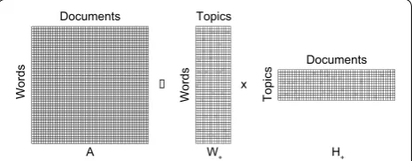
Term frequency‑inverse document frequency (TF‑IDF) The term-document matrix, denoted as A, plays a cen-tral role in our analysis (see Manning et al. 2008). Each row of A corresponds to a unique word in the vocabu-lary, and each column of A corresponds to a document (Fig. 1). The (i, j)th entry of A is the term frequency (TF) of the ith word appearing in the jth document. Note that the term-document matrix ignores the ordering of words in the documents. Following convention, the (i, j)th entry of A is the inverse document frequency (IDF) weighting for each term in the vocabulary (Manning et al. 2008). This weighting scheme puts less weight on the terms that appear in more documents and more weight on terms appear infrequently in documents. The premise is that common terms have less discriminative power relative to rare words.
Topic discovery non‑negative matrix factorization (NMF) We focus on a particular linear algebraic method in unsu-pervised machine learning for topic discovery, namely nonnegative matrix factorization (NMF) (Lee and Seung 1999). The linear algebraic approach is computationally efficient and scalable to massive data sets, for example
H
A W+ +
Documents
Word
s
Topics
Topics
x
Documents
Word
s
Fig. 1 Conceptual illustration of non-negative matrix factorization (NMF) decomposition of a matrix consisting of m words in n docu-ments into two non-negative matrices of the original m words by k
the text descriptions of nearly one million crimes dis-cussed below. The linear algebraic approach contrasts with probabilistic methods such as the popular latent Dirichlet allocation (LDA) (Blei et al. 2003), which is computationally expensive. Our approach does not yield a probabilistic interpretation and rigorously should be called a “document clustering” method. Recent research, however, has built connections between linear algebraic and probabilistic methods for topic modeling (Arora et al. 2013), supporting the usefulness of linear algebraic methods as an efficient way to compute topic models.
NMF is designed for discovering interpretable latent components in high-dimensional unlabeled data such as the set of documents described by the counts of unique words. NMF uncovers major hidden themes by recast-ing the term-document matrix A into the product of two other matrices, one matrix representing the relation-ships between words and topics and another represent-ing the relationship between topics and documents in the latent topic space (Fig. 1) (Xu et al. 2003). In particular, we would like to find matrices W ∈Rm+×k and H∈R
k×n
+
to solve the approximation problem A ≈ WH, where R+ is the set of all nonnegative numbers and m, n and k are the numbers of unique words, documents, and topics, respectively. The term-document matrix A is given as the input, while W and H enclose the latent term-topic and topic-document information. Specifically, W reflects the frequency of different words in each discovered topic, while H reflects the topic mix present in each document. Note that the number of topics k is typically many orders of magnitude smaller than the number of words m and number of documents n under consideration and thus topic modeling is a form of dimension reduction. Matri-ces W and H constitute the principal result of topic mod-eling and the distribution of words and documents in relation to topics is the primary focus of interpretation.
Numerous algorithms exist for solving A ≈ WH
(Cichocki et al. 2009; Kim et al. 2014). A general approach is to measure the difference between A and WH
(Kim et al. 2014):
where �·�F is the Frobenius norm. A good topic model is one that minimizes the squared difference between the raw data contained in the term-document matrix A
and product of candidate term-topic and document-topic matrices, W and H. The problem resembles a least-squares formulation and indeed a common solution approach relies on a non-negative least squares method. The optimization is computed iteratively by alternat-ing between minimization given candidate entries of W
(1)
min W,H>0�A−
WH�2F
and then given candidate entries for H (Kuang and Park 2013):
This approach would take several hours to run on large-scale data sets consisting of millions of documents, which is the challenge we face here. We therefore employ a highly efficient hierarchical rank-2 NMF algorithm that is orders of magnitude faster (Kuang and Park 2013). The algorithm first constructs a hierarchy of topics in the form of a binary tree. Each node in the tree is scored on the basis of how distinctive it is as a topic from its sis-ter and a node is no longer split if two well-differentiated daughters can no longer be found. Terminal leaf nodes of the tree are chosen to represent the flat topic model. Details of the algorithmic process are presented in (Kuang and Park 2013).
In theory, hierarchical rank-2 NMF could proceed to produce hundreds or thousands of topics depend-ing on the size of the corpus of documents. Obviously, this would defeat the purpose of trying to reduce the dimensionality of the problem to a relatively small set of interpretable topics. One option is to set a relatively high threshold in the scoring system which then natu-rally terminates when all of the existing nodes in a tree can no longer be split to form well-differentiated topics (Kuang and Park 2013). We simply choose the maximum number of terminal nodes to be 20. Comparison with 50 and 100 topic models finds little additional meaningful differentiation.
Cosine similarity and crime type clusters
Text-based topic modeling typically reveals that any one document is a mixture of different topics. Therefore, in principle, the distance between any two documents can be measured by comparing how far apart their topic mixture distributions are. Here we extend this idea to consider officially recognized crime types as mixtures of different crime topics. The distance between any two official crime types can be measured using the topic mixtures observed for those two crime types. We use cosine similarity (Steinbach et al. 2000) to compute such measures.
Consider two hypothetical crime types A and B. Type
A might represent aggravated assault and type B might represent residential burglary. Each crime type is a col-lection of many individual events, each of which is poten-tially a mixture of one or more crime topics. To simplify
(2)
min
W>0
W
THT −AT
2
F,
(3) min
H>0�
analysis, we assign each crime event to its dominant topic, defined as the topic which shares the greatest over-lap in words with the narrative text for the crime. After assigning crimes to individual topics, inspection of all of the events formally classified as assault with a deadly weapon might show that 40% fall into crime topic i = 1, 30% fall into topic 4, 20% into topic 9, and 10% into topic 12. Similarly, for all the events formally classified as resi-dential burglary, 5% might fall into topic i = 9, 15% into topic 12, 60% into topic 15 and 20% into topic 19. Assault with a deadly weapon and residential burglary are similar only in events falling into topics 9 and 12. More formally, the similarity between any two official crime types A and
B is given as:
where Ai is the frequency at which events formally clas-sified as crime type A belongs to topic i and equivalently for events formally classified as crime type Bi.
We choose cosine similarity over other measures such as KL-divergence and Chi square distances because cosine similarity is bounded, taking values between − 1 and 1, and is a good measure for graph-based crime type clustering (discussed below). Negative values reflect dis-tributions that are increasingly diametrically opposed and positive values distributions that point in the same direction. Values of cosine similarity near zero reflect vectors that are uncorrelated with one another. In our case, cosine similarity will only assume values between 0 and 1 because NMF returns only positive valued matrices.
Viewing the collection of official crime types as a graph, where each crime type is a node and cosine sim-ilarities define the weights of the edges between nodes, we use average linkage clustering (Legendre and Leg-endre 2012) on this graph to partition the crime types into ecologically meaningful groups (see also Brennan
cos(θ )=
k i=1AiBi
k i=1A2i
k
i=1B2i
1987: 228). Crime types are clustered in an agglom-erative manner. Initially, each crime type exists as its own isolated cluster. The two closest clusters are then merged in a recursive manner, with the new cluster adopting the mean similarity from all cluster mem-bers. The process continues until only C clusters are left. The number C can be chosen automatically by a cluster validation method such as predictive strength (Tibshirani and Walther 2005), or manually for eas-ier interpretation. We manually set the number of clusters.
Data and analysis plan
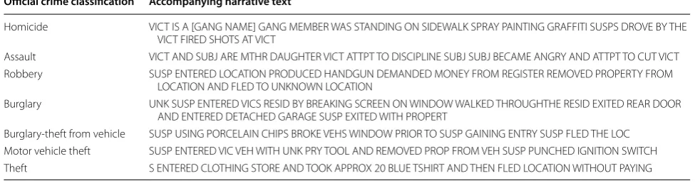
The above modeling framework is flexible enough in principle to handle any form of data (e.g., Chen et al. 2010), not just text. In spite of this flexibility, we do not stray far from its most common application in text min-ing. Here we exploit the presence of short text descrip-tions associated with individual crime events to compute text-based hierarchical NMF. Table 1 illustrates several examples of individual crime events and the associated text descriptions of the events.
We focus on the complete set of crimes reported to the Los Angeles Police Department (LAPD) from Janu-ary 1, 2009 and July 19, 2014. The end date of the sample is arbitrary. Los Angeles is a city of approximately 4 mil-lion people occupying an area of 503 square miles. The Los Angeles Police Department is solely responsible for policing this vast area, though Los Angeles is both sur-rounded by and encompasses independent cities with their own police forces.
The total number of reported crimes handles by the LAPD during the sample period was 1,027,168. In a typi-cal year, the LAPD collected reports on 180,000 crimes. On average 509 crimes were recorded per day, with crime reports declining over the entire period. During the first year of the sample, LAPD recorded on average 561.5 crimes per day. During the last year they recorded 463.8 crimes per day.
Table 1 Examples of official crime classifications and the narrative text tied to the event
Official crime classification Accompanying narrative text
Homicide VICT IS A [GANG NAME] GANG MEMBER WAS STANDING ON SIDEWALK SPRAY PAINTING GRAFFITI SUSPS DROVE BY THE VICT FIRED SHOTS AT VICT
Assault VICT AND SUBJ ARE MTHR DAUGHTER VICT ATTPT TO DISCIPLINE SUBJ SUBJ BECAME ANGRY AND ATTPT TO CUT VICT Robbery SUSP ENTERED LOCATION PRODUCED HANDGUN DEMANDED MONEY FROM REGISTER REMOVED PROPERTY FROM
LOCATION AND FLED TO UNKNOWN LOCATION
Burglary UNK SUSP ENTERED VICS RESID BY BREAKING SCREEN ON WINDOW WALKED THROUGHTHE RESID EXITED REAR DOOR AND ENTERED DETACHED GARAGE SUSP EXITED WITH PROPERT
The crime coding system used by the LAPD includes 226 recognized crime types. This is considerably more finely resolved than either the FBI Uniform Crime Reports (7 Part I and 21 Part II offenses), or National Inci-dent Based Reporting System (49 Group A and 90 Group B offenses). Aggravated assault, for example, is associ-ated with four unique crime codes including assault with a deadly weapon, assault with a deadly weapon against a police officer, shots fired at a moving vehicle, and shots fired at a dwelling. These crime types could be considered a type of ground truth against which topic model classifi-cations can be evaluated. We are interested in the degree of alignment of the LAPD crime types and topic models derived from text-based narratives accompanying those crimes.
In addition to this rich coding system, a large fraction of the incidents recorded in the sample include narra-tive text of the event. Of the 1,027,168 recorded crimes, 805,618 (78.4%) include some form of text narrative. On average 397.6 events per day contain some narrative text describing the event. The fraction of events containing narrative text increased over time from 76.6% of events, in the first 6 months of the sample, to 87.0%, in the last 6 months.
There are pointed differences in the occurrence of nar-rative text by official crime types (Table 2). Virtually all violent crimes are accompanied by narrative text. Rob-bery and homicide have associated narrative text for 98.9 and 98.2% of events, respectively. Assault and kidnapping have 97.8 and 97.4% of events associated with narrative text. Burglary shows narrative text occurrence on par with the most serious violence crimes (98.6%). For less serious property crimes, narrative text reporting falls off to 91.1% for theft and 74.3% for vandalism. The lowest occurrence of narrative text is seen for arson (37.8%) and motor vehicle theft (4.3%). In the former case, it must be
acknowledged that most arson reporting responsibilities lie with the fire department, so low narrative load might be expected. In the latter case, either the vehicles are not recovered (about 40% of the cases) and therefore the cumstances of the theft are not known, or detailed cir-cumstances beyond make, model and year of the car—all recorded in separate fields—are not deemed as relevant to recording of the crime.
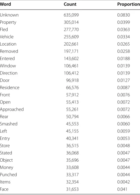
Overall, the text narratives associated with crime events total 7,649,164 discrete words, after preprocess-ing (see above). These are unevenly distributed across events. The mean number of words contained in a single narrative is 18.57 (s.d. 6.72), while the maximum num-ber of words is 41 (see Table 1). Individual words are also unevenly distributed, though not massively so (Table 3). For example, the word “unknown” is the most common word in the corpus appearing 635,099 times. However, this still represents only 8.3% of all words. The next most common word is “property” occurring 305,014 times, but represents only 4% of all words. Words that are strongly indicative of crime type are extremely rare. The word homicide appears only 45 times in the entire text corpus, a frequency of 5.88 × 10⁻⁶ overall. Burglary appears 252
times, robbery 286 times, assault 457 times, and theft 969 times. When they do appear, diagnostic words are not generally coincident with the corresponding formal classifications. For example, of the 1593 formally clas-sified homicides in the dataset, only 11 of those events also find the word homicide as part of the narrative text. Thus, 1582 formally classified homicides are not explic-itly marked as such in the narrative text. The 34 events that include the word homicide in the narrative, but are not classified as homicides, include 17 events labeled as “other” (primarily threatening letters or phone calls), nine aggravated assaults, seven vandalism events, and one robbery. In general, narrative text provides context rather
Table 2 Counts of events with and without accompanying narrative text by official crime type
No narrative text Narrative text Total Fraction with narrative text
Robbery 597 53,379 53,976 0.989
Burglary 1320 91,260 92,580 0.986
Homicide 28 1565 1593 0.982
Assault 1032 45,665 46,697 0.978
Kidnapping 45 1707 1752 0.974
Grand theft person 230 7754 7984 0.971
Theft 13,326 136,117 149,443 0.911
Burglary-theft from vehicle 20,192 126,912 147,104 0.863
Other miscellaneous crime 72,518 256,816 329,334 0.780
Vandalism 27,630 80,038 107,668 0.743
Arson 1111 675 1786 0.378
than strictly redundant typological detail. It is important to note, however, that narrative text and formal crime type classifications are unlikely to be completely decou-pled. Ultimately, it is the job of police officers in the field to recognize and record behavioral and circumstantial evidence consistent with legal definitions of different crime types. Thus we should expect that specific narrative words correlate to some degree with formally recognized crime types. As a result, we may also expect there to be important differences across crime types in the character of their associated narrative text. Such variation could be explored further with text-based topic modeling.
Results
Hierarchical models for all crimes
Figure 2 presents a hierarchical topic model applied to all crime events in the LAPD corpus associated with narrative text. After preprocessing the data set includes 711,119 events. Each node in the tree represents a latent topic characterized by key words appearing in the topic. Summary statistics for the number of events, the percent violent and property crime, and the top-ten words for
each topic node are shown in tabular format. The hier-archical structure is shown in graph form. Terminal leaf nodes are highlighted in gray.
The topic tree has three major components. The topics associated with the left branch (Nodes A–O) are linked to property crimes (Fig. 2). Words such as property and
vehicle identify key targets of crime, while words such
as window, door, enter, remove, and fled describe the
behavioral steps or sequences involved in commission of a crime. The validity of the property crime label for this component may be tested by using the formally recog-nized crime types in the LAPD ground truth. For exam-ple, 93.4% of the events associated with terminal leaf node C are formally recognized by the LAPD as prop-erty crimes. None of the intermediate or terminal nodes in the left branch (Nodes A–O) captures less than 89.9% property crimes.
By contrast, the right branch (Nodes P-AG) stands out for its connection to violent crime (Fig. 2). Words such as face, head and life identify key targets of crime, while words such as approach, verbal, and punch iden-tify sequences of behaviors involved in violent actions. The LAPD ground truth supports the broad label of topics P-AG as violent crime. For example, 90.5% of all the events associated with terminal topic S are formally recognized as violent crime types. With the exception of nodes P and Y, no other topic in this component captures less than 70% of formally recognized violent crimes. Ter-minal node Y appears to be an association of violations of court orders and/or annoying communications, which may be reasonable ecological precursors to or conse-quences of other violent crimes.
Intermediate node P is a bridge between crime top-ics that are clearly associated with violent crime (Nodes Q-AG) and a series of crime topics we label as deception-based property crime (Nodes AH-AL). Words indica-tive of shoplifting and credit card fraud stand out in this group of topics. Why such topics trace descent through a branch more closely with violent is unclear.
Hierarchical models for aggravated assault and homicide Figure 3 presents topic modeling results for the sub-set of crimes formally classified by the LAPD as aggra-vated assaults (LAPD code 230) and homicide (LAPD code 110). This is a semi-supervised analysis in the sense that we have used information external to narrative data to partition or stratify the collection of events into a priori groups. Our goal is to assess topic distinctions that arise within these serious violent crimes. A total of 40,208 events are classified as either aggravated assaults (38,626 events) or homicides (1582 events). Notion-ally, these events are separated on the basis of outcome (i.e., death), but such a distinction is not visible within
Table 3 The top twenty-five most common words in the full
text corpus consisting of 7,649,164 discrete words
Word Count Proportion
Unknown 635,099 0.0830
Property 305,014 0.0399
Fled 277,770 0.0363
Vehicle 255,609 0.0334
Location 202,661 0.0265
Removed 197,171 0.0258
Entered 143,602 0.0188
Window 106,461 0.0139
Direction 106,412 0.0139
Door 96,918 0.0127
Residence 66,576 0.0087
Front 57,912 0.0076
Open 55,413 0.0072
Approached 55,261 0.0072
Rear 50,794 0.0066
Smashed 45,553 0.0060
Left 45,155 0.0059
Entry 40,341 0.0053
Store 36,515 0.0048
Stated 36,068 0.0047
Object 35,696 0.0047
Money 33,608 0.0044
Punched 33,317 0.0044
Items 32,354 0.0042
the classification hierarchy. Rather, the key distinction is between topics involving weapons other than firearms (Nodes A–I) and those involving firearms (Nodes J–R). Homicide looms large in terms of legal and harm-based classification (Ratcliffe 2015; Sherman 2011), and plays a
large role in public health debates (Cook et al. 2017; Jena et al. 2014), but it is not resolved within the larger volume of aggravated assaults. Homicides never make up more than 2.1% of any of the non-gun violence topics (Nodes A–I) (Fig. 3). Homicides never rise above 11.8% in the Fig. 2 Hierarchical NMF topic structure for the entire corpus of events. The left branch captures property crimes. The right branch captures violent crimes. Deception-based property crimes form a distinct tree in the right branch. Tables show topic labels, number of events in each topic, number of events of the top 40 most frequent crime types in each topic, the percent of events for the topic that are formally classified as violent crime (v%) or property crime (p%), and the top-ten topic words. Terminal leaves of the topic model are marked in gray
gun violence topics (Nodes J–R). Notably, the greater lethality of guns is clearly visible when comparing the percent of homicides that are gun-related and those that are not. The most lethal crime topic is terminal node N, with key words approach, handgun, multiple, shot, and
fled. Node P stands out with an emphasis on the use of vehicles as a weapon, but still tracing a pattern of descent linked to gun violence. Inspection of the top 100 words in this topic confirms that gun-related terms do not appear in topic P. The close connection to topic Q, which links guns and vehicles, is clearly through the common ele-ment of vehicles not guns.
Figure 4 shows that removing homicides from the sub-set of events does not fundamentally change the structure of the resulting topics. Indeed, it seems clear that assaults provide the overriding structure for crimes of interper-sonal violence. This outcome may reflect the relatively low volume of homicides relative to aggravated assaults, but also the fact that homicides and aggravated assaults are ecologically very closely related (Goldstein 1994). Topic nodes A–I are notable for making fine-grained dis-tinctions between the targets of violence, including head,
face, hand, and arm, the weapons used, including metal
object, bottle, and knife, and the action, including hit,
threw, punch, kick, stab, and cut. The topics appear
tacti-cally very exacting. For example, the topics consistently show knives being used to target the body, while bottles/ blunt object are used to target the head (Ambade and Godbole 2006; Webb et al. 1999).
Hierarchical model for homicides
Figure 5 presents the results of hierarchical NMF analy-sis of text narratives associated with formally classi-fied homicides. There are clear distinctions that surface within formally classified homicides in spite of the much smaller numbers of events (1414 with more than three words). The primary split is between homicides involving firearms (Node A and all of its daughters) and those where firearms are not indicated (Node R). Node R in fact features words stab and head, which we know from the broader analysis of aggravated assaults are two terms associated with knife violence and blunt-force violence, respectively (see Figs. 3, 4). Node H implicate
gangs exclusively in relation to gun violence. Nodes D,
F and G highlight the central role of vehicles in gun vio-lence. In each of these latter topics, words showing peo-ple emerging to attack or being attacked in cars, lending much behavioral and situational nuance to gun violence. By contrast, the adjacent branch (Nodes I–Q) appears to capture street-based homicides where the offender
approached and fled on foot.
Crimes as mixtures of topics
The above discussion points to key terms such as knife,
different topics. This observation leads to a conceptual-ization of crimes as mixtures of crime different topics.
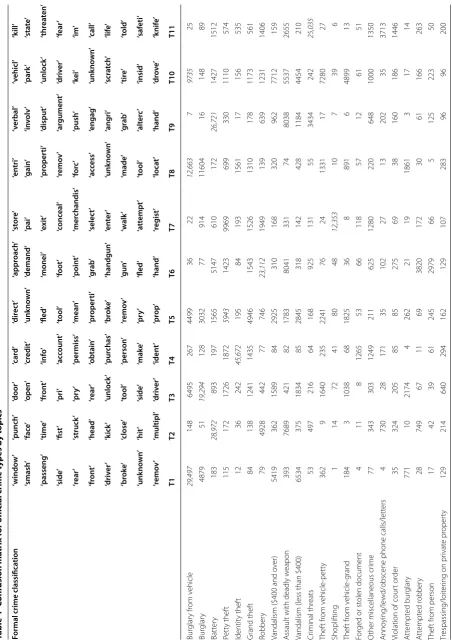
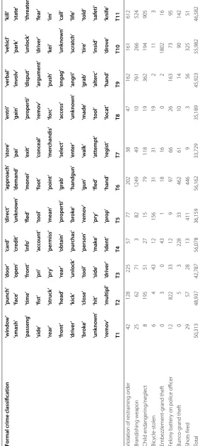
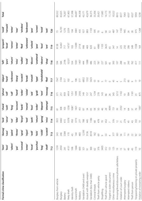
Table 4 shows a confusion matrix for formal crime types assigned by the LAPD against the topics associated with each crime event. A confusion matrix is typically used for evaluating the performance of a predictive algo-rithm (Fielding and Bell 1997). Here a confusion matrix is used to illustrate both how official crime types exist as mixtures of topics and how individual topics are associ-ated with many different official crime types. We use a refined version of the leaf nodes from hierarchical clus-tering for all crime types and number the topics from 1 to 20 (see Fig. 2). We also restrict the confusion matrix to the thirty most common crime types in the dataset for readability. Clustering analyses below restrict the analysis to the forty most common crime types.
Official crime types mix topics in unique ways. Row counts in Table 4 give the number of events of a given offi-cial crime type that are assigned to different discovered crime topics. Recall that each crime event can be a mix-ture of different topics. However, we assign each event to a single topic based on overlap in narrative text words. Using this procedure, for example, 29,497 (32.94%) of the 89,552 events officially classified by the LAPD as burglary from vehicle are assigned to Topic 1. This topic is marked by words smash/broke, rear/passenger/side/driver/fron
t, window, and remove, all of which provide clear target
and behavioral information intuitively consistent with the official crime type. However, other topics also grab sig-nificant numbers of burglary from vehicle events. Topics 3 (7.25%), 5 (5.02%), 8 (14.14%), 10 (10.87%), 14 (8.79%),
and 19 (9.09%) each represent at least 5% of total events (Table 4). Topic 8 shares a connection on property crime with Topic 1, but otherwise emphasizes a very different focus, marked by words such as force/gain, access/entry,
tool, remove and property. Topic 8 sounds considerably
more generic and is consistent with burglary in general. Similarly, Topic 10 also grabs a large number of burglary from vehicle events, but here the focus is more clearly on vandalism, marked by words such as kei ([sic] i.e., key),
scratch and tire. A more formal analysis of mixture
char-acteristics is presented below.
Topic mixtures also characterize violent crimes. For example, aggravated assault (or assault with a deadly weapon) has events distributed evenly across Topics 2 (7689 events or 18.02%), 6 (8041 events, 18.84%) and 9 (8038 events, 18.83%). Topic 2 is characterized by words such as punch/kick, hit/struck, face/head, without promi-nent occurrence of words related to weapons. Topic 6, by contrast, features words such as gun/handgun as well as
approach, demand and money. Topic 9 involves words
such as verbal, argument/dispute, grab, push, and hand. While aggravated assaults appear to be evenly divided among these three topics, the topics themselves suggest heterogeneity in crime contexts. Topic 8 clearly stands out as related to robbery.
Crime topics are also not exclusively linked to individ-ual crime types (Table 4). Rather single topics are spread across crime types at different frequencies. For example, 58.63% (24,497) of the Topic 1 events fall within burglary from vehicle. However, 12.99, 10.77 and 9.7% of Topic 1 events are classified as petty vandalism under $400,
Table
4
C
onfusion ma
trix f
or official crime t
yp
es b
y t
opics
Formal crime classifica
tion ‘windo w ’ ‘punch ’ ‘door ’ ‘car d’ ‘dir ec t’ ‘appr oach ’ ‘st or e’ ‘en tri ’ ‘v erbal ’ ‘v ehicl ’ ‘k ill ’ ‘smash ’ ‘fac e’ ‘open ’ ‘cr edit ’ ‘unk no wn ’ ‘demand ’ ‘pai ’ ‘gain ’ ‘in volv ’ ‘park ’ ‘s tate ’ ‘passeng ’ ‘time ’ ‘fr on t’ ‘inf o’ ‘fled ’ ‘monei ’ ‘e xit ’ ‘pr oper ti ’ ‘disput ’ ‘unlock ’ ‘thr ea ten ’ ‘side ’ ‘fist ’ ‘pri ’ ‘ac coun t’ ‘tool ’ ‘foot ’ ‘c onc eal ’ ‘remo v’ ‘ar gumen t’ ‘driv er ’ ‘fear ’ ‘rear ’ ‘struck ’ ‘p ry ’ ‘permiss ’ ‘mean ’ ‘poin t’ ‘mer chandis ’ ‘fo rc ’ ‘push ’ ‘ke i’ ‘im’ ‘fr on t’ ‘head ’ ‘rear ’ ‘obtain ’ ‘pr oper ti ’ ‘g ra b’ ‘selec t’ ‘ac cess ’ ‘engag ’ ‘unk no wn ’ ‘call ’ ‘driv er ’ ‘k ick ’ ‘unlock ’ ‘pur chas ’ ‘br ok e’ ‘handgun ’ ‘en ter ’ ‘unk no wn ’ ‘ang ri ’ ‘scr at ch ’ ‘lif e’ ‘br ok e’ ‘close ’ ‘tool ’ ‘person ’ ‘remo v’ ‘gun ’ ‘w alk ’ ‘made ’ ‘g ra b’ ‘tir e’ ‘told ’ ‘unk no wn ’ ‘hit ’ ‘side ’ ‘m ak e’ ‘p ry ’ ‘fled ’ ‘a tt empt ’ ‘tool ’ ‘alt er c’ ‘insid ’ ‘saf eti ’ ‘remo v’ ‘multipl ’ ‘driv er ’ ‘iden t’ ‘pr op ’ ‘hand ’ ‘reg ist ’ ‘loca t’ ‘hand ’ ‘d ro ve ’ ‘k nif e’ T1 T2 T3 T4 T5 T6 T7 T8 T9 T10 T11 Bur glar y fr om v ehicle 29,497 148 6495 267 4499 36 22 12,663 7 9735 25 Bur glar y 4879 51 19,294 128 3032 77 914 11604 16 148 89 Batt er y 183 28,972 893 197 1565 5147 610 172 26,721 1427 1512 Pett y thef t 115 172 1726 1872 5943 1423 9969 699 330 1110 574 Identit y thef t 12 36 242 45,672 195 84 193 1561 17 156 535 Grand thef t 84 138 1241 1435 4946 1543 1526 1310 178 1173 561 Robber y 79 4928 442 77 746 23,112 1949 139 639 1231 1406
Vandalism ($400 and o
ver) 5419 362 1589 84 2925 310 168 320 962 7712 159 A
ssault with deadly w
eapon 393 7689 421 82 1783 8041 331 74 8038 5537 2655
Vandalism (less than $400)
6534 375 1834 85 2845 318 142 428 1184 4454 210 Cr iminal thr eats 53 497 216 64 168 925 131 55 3434 242 25,035 Thef t fr om v ehicle -pett y 362 9 1640 235 2241 76 24 1331 17 7280 27 Shoplif ting 1 14 72 41 80 48 12,353 10 7 39 6 Thef t fr om v ehicle -g rand 184 3 1038 68 1825 36 8 891 6 4899 13 For
ged or st
olen document 4 11 8 1265 53 66 118 57 12 61 51 O
ther miscellaneous cr
ime 77 343 303 1249 211 625 1280 220 648 1000 1350 Anno ying/le w
d/obscene phone calls/lett
ers 4 730 28 171 35 102 27 13 202 35 3713
Violation of cour
t or der 35 324 205 85 85 275 69 38 160 186 1446 A tt empt ed bur glar y 771 10 2174 4 262 21 19 1861 3 17 14 A tt empt ed r obber y 28 749 67 11 69 3820 172 30 61 166 263 Thef t fr om person 17 42 39 61 245 2979 66 5 125 223 50 Tr espassing/loit er
ing on pr
Table
4
c
on
tinued
Formal crime classifica
tion ‘windo w ’ ‘punch ’ ‘door ’ ‘car d’ ‘dir ec t’ ‘appr oach ’ ‘st or e’ ‘en tri ’ ‘v erbal ’ ‘v ehicl ’ ‘k ill ’ ‘smash ’ ‘fac e’ ‘open ’ ‘cr edit ’ ‘unk no wn ’ ‘demand ’ ‘pai ’ ‘gain ’ ‘in volv ’ ‘park ’ ‘s tate ’ ‘passeng ’ ‘time ’ ‘fr on t’ ‘inf o’ ‘fled ’ ‘monei ’ ‘e xit ’ ‘pr oper ti ’ ‘disput ’ ‘unlock ’ ‘thr ea ten ’ ‘side ’ ‘fist ’ ‘pri ’ ‘ac coun t’ ‘tool ’ ‘foot ’ ‘conc eal ’ ‘remo v’ ‘ar gumen t’ ‘driv er ’ ‘fear ’ ‘rear ’ ‘struck ’ ‘p ry ’ ‘permiss ’ ‘mean ’ ‘poin t’ ‘mer chandis ’ ‘fo rc ’ ‘push ’ ‘ke i’ ‘im’ ‘fr on t’ ‘head ’ ‘rear ’ ‘obtain ’ ‘pr oper ti ’ ‘g ra b’ ‘selec t’ ‘ac cess ’ ‘engag ’ ‘unk no wn ’ ‘call ’ ‘driv er ’ ‘k ick ’ ‘unlock ’ ‘pur chas ’ ‘br ok e’ ‘handgun ’ ‘en ter ’ ‘unk no wn ’ ‘ang ri ’ ‘scr at ch ’ ‘lif e’ ‘br ok e’ ‘close ’ ‘tool ’ ‘person ’ ‘remo v’ ‘gun ’ ‘w alk ’ ‘made ’ ‘g ra b’ ‘tir e’ ‘told ’ ‘unk no wn ’ ‘hit ’ ‘side ’ ‘m ak e’ ‘p ry ’ ‘fled ’ ‘a tt empt ’ ‘tool ’ ‘alt er c’ ‘insid ’ ‘saf eti ’ ‘remo v’ ‘multipl ’ ‘driv er ’ ‘iden t’ ‘pr op ’ ‘hand ’ ‘reg ist ’ ‘loca t’ ‘hand ’ ‘d ro ve ’ ‘k nif e’ T1 T2 T3 T4 T5 T6 T7 T8 T9 T10 T11
Violation of r
estraining or der 42 128 225 57 77 202 38 47 162 161 612 Brandishing w eapon 25 62 71 3 82 1249 49 10 761 266 524 Child endanger ing/neglec t 8 195 51 27 15 79 118 19 362 194 905 Bic ycle -st olen 6 4 43 12 156 31 31 19 2 11 3 Embezzlement -g rand thef t 0 3 0 43 1 18 16 0 2 1802 16 Felon y batt er
y on police officer
Table
4
c
on
tinued
Formal crime classifica
tion ‘it em ’ ‘damag ’ ‘lock ’ ‘check ’ ‘phone ’ ‘objec t’ ‘lef t’ ‘pr oper ti ’ ‘resid ’ Total ‘busi ’ ‘caus ’ ‘secur ’ ‘cash ’ ‘c ell ’ ‘har d’ ‘purs ’ ‘loca t’ ‘ransack ’ ‘selec t’ ‘pain t’ ‘cut ’ ‘fo rg ’ ‘call ’ ‘unk no wn ’ ‘return ’ ‘remo v’ ‘en ter ’ ‘pai ’ ‘thr ew ’ ‘bik e’ ‘ac coun t’ ‘hand ’ ‘sharp ’ ‘miss ’ ‘en ter ’ ‘rear ’ ‘c onc eal ’ ‘spr ai ’ ‘bic ycl ’ ‘bank ’ ‘or der ’ ‘scr at ch ’ ‘w allet ’ ‘fled ’ ‘windo w ’ ‘en ter ’ ‘injuri ’ ‘tool ’ ‘monei ’ ‘viola t’ ‘br eak ’ ‘insid ’ ‘unk no wn ’ ‘bedr oom ’ ‘loca t’ ‘w all ’ ‘park ’ ‘busi ’ ‘ask ’ ‘smash ’ ‘disc ov ’ ‘unlock ’ ‘p oe’ ‘pur chas ’ ‘k ick ’ ‘return ’ ‘or der ’ ‘g ra b’ ‘type ’ ‘una tt end ’ ‘p oe’ ‘scr een ’ ‘bag ’ ‘visibl ’ ‘gar ag ’ ‘deposit ’ ‘tex t’ ‘windshield ’ ‘obser v’ ‘busi ’ ‘insid ’ ‘shelf ’ ‘scr at ch ’ ‘miss ’ ‘a tt empt ’ ‘messag ’ ‘fled ’ ‘shop ’ ‘e nt ’ ‘e xit ’ T12 T13 T14 T15 T16 T17 T18 T19 T20 Bur glar y fr om v ehicle 1239 243 7872 81 371 7547 594 8138 73 89,552 Bur glar y 2050 246 4482 308 251 1704 584 16,463 16,705 83,025 Batt er y 241 5384 415 103 959 517 2196 717 1276 79,207 Pett y thef t 4131 170 5378 1258 4914 102 10,521 14737 2259 67,403 Identit y thef t 598 43 950 5087 1251 5 554 103 104 57,398 Grand thef t 1666 144 3773 1821 1099 108 5581 13289 3081 44,697 Robber y 669 483 277 451 2593 577 1407 2718 435 44,358
Vandalism ($400 and o
ver) 321 12,595 788 87 149 6852 444 998 927 43,171 A
ssault with deadly w
eapon 91 3136 445 34 157 1332 1088 469 883 42,679
Vandalism (less than $400)
300 8318 1186 83 247 5423 486 820 1103 36,375 Cr iminal thr eats 62 182 68 58 1234 53 223 61 595 33,356 Thef t fr om v ehicle -pett y 376 69 478 50 278 91 787 4980 70 20,421 Shoplif ting 3405 9 70 46 143 5 227 1103 6 17,685 Thef t fr om v ehicle -g rand 312 53 452 28 96 77 501 3625 58 14,173 For
ged or st
olen document 151 4 7 9099 26 0 45 65 32 11,135 O
ther miscellaneous cr
ime 125 377 376 721 345 45 393 347 487 10,522 Anno ying/le w
d/obscene phone calls/lett
ers 19 301 12 39 3212 4 107 14 147 8915
Violation of cour
t or der 15 56 21 2592 1102 5 288 225 1165 8377 A tt empt ed bur glar y 37 111 274 14 10 213 33 250 945 7043 A tt empt ed r obber y 49 79 45 64 304 85 243 206 26 6537 Thef t fr om person 45 22 43 37 1181 9 762 548 28 6527 Tr espassing/loit er
ing on pr
ivat e pr oper ty 119 92 332 76 23 17 417 1558 975 5959
Violation of r
Table
4
c
on
tinued
Formal crime classifica
tion ‘it em ’ ‘damag ’ ‘lock ’ ‘check ’ ‘phone ’ ‘objec t’ ‘lef t’ ‘pr oper ti ’ ‘resid ’ Total ‘busi ’ ‘caus ’ ‘secur ’ ‘cash ’ ‘c ell ’ ‘har d’ ‘purs ’ ‘loca t’ ‘ransack ’ ‘selec t’ ‘pain t’ ‘cut ’ ‘fo rg ’ ‘call ’ ‘unk no wn ’ ‘return ’ ‘remo v’ ‘en ter ’ ‘pai ’ ‘thr ew ’ ‘bik e’ ‘ac coun t’ ‘hand ’ ‘sharp ’ ‘miss ’ ‘en ter ’ ‘rear ’ ‘c onc eal ’ ‘spr ai ’ ‘bic ycl ’ ‘bank ’ ‘or der ’ ‘scr at ch ’ ‘w allet ’ ‘fled ’ ‘windo w ’ ‘en ter ’ ‘injuri ’ ‘tool ’ ‘monei ’ ‘viola t’ ‘br eak ’ ‘insid ’ ‘unk no wn ’ ‘bedr oom ’ ‘loca t’ ‘w all ’ ‘park ’ ‘busi ’ ‘ask ’ ‘smash ’ ‘disc ov ’ ‘unlock ’ ‘p oe’ ‘pur chas ’ ‘k ick ’ ‘return ’ ‘or der ’ ‘g ra b’ ‘type ’ ‘una tt end ’ ‘p oe’ ‘scr een ’ ‘bag ’ ‘visibl ’ ‘gar ag ’ ‘deposit ’ ‘tex t’ ‘windshield ’ ‘obser v’ ‘busi ’ ‘insid ’ ‘shelf ’ ‘scr at ch ’ ‘miss ’ ‘a tt empt ’ ‘messag ’ ‘fled ’ ‘shop ’ ‘e nt ’ ‘e xit ’ T12 T13 T14 T15 T16 T17 T18 T19 T20 Brandishing w eapon 8 38 31 3 21 19 70 37 115 3444 Child endanger ing/neglec t 10 264 19 49 21 10 413 76 402 3237 Bic ycle -st olen 3 3 1365 1 1 8 151 401 58 2309 Embezzlement -g rand thef t 0 1 0 10 31 0 279 1 1 2224 Felon y batt er
y on police officer
3 381 6 30 8 10 137 19 5 2007 Bunco -g rand thef t 19 6 7 575 123 0 33 64 44 1919 Shots fir ed 3 91 6 5 0 7 44 117 75 1776 Total 17,012 34,995 30,147 25,571 22,355 25416 30,630 74,287 35441 D ominan t w or
ds in each t
opic ar
e sho
wn acr
oss the t
op
. R
ow t
otals r
eflec
t the t
otal number of cr
imes f
or
mally classified under each cr
ime t ype . C olumn t otal r eflec
t the t
otal number of cr
imes clust
er
ed within each t
opic
.
Italic numbers ar
e c
vandalism over $400 and burglary, respectively. Topic 1 thus reveals connections among three different crime types. Such is the case for each topic. For example, 14.3% (8041) of Topic 6 events are aggravated assaults, though robbery is the single most common crime type attributed to this topic (41.15% or 23,112 events). Battery (9.17% or 5147 events), attempted robbery (6.8% or 3820 events) and theft from person (5.3% or 2979 events) are all also heavily represented within Topic 6.
Overall, the confusion matrix gives the sense that crimes may be related to one another in subtle ways and that these subtle connections can be discovered in the narrative descriptions of those events. A more for-mal way to consider such connections is to measure the similarities in their topic mixtures. The premise is that two crime types are more similar to one another if their distribution of events over topics is similar. For example,
burglary from vehicle and petty vandalism show simi-lar relative frequencies of events within Topic 3 (7.3 and 5.0%, respectively), Topic 5 (5.0 and 7.8%) and Topic 10 (10.9 and 12.2%) (Table 4). This gives the impression that burglary from vehicle and petty vandalism are closely related to one another.
Distances between crime types and crime topic clustering To develop a more quantitative understanding of the relationships among formally recognized crime types we turn to the cosine similarity metric (Steinbach et al. 2000). Figure 6 shows the cosine similarity between for-mally recognized crime types as a matrix plot where the gray-scale coloring reflects the magnitude of similarity. The matrix is sorted in descending order of similarity. The darkest matrix entries are along the diagonal, reflect-ing the obvious point that any one crime type is most
similar to itself in the distribution of events across topics. More revealing is the ordering of crime types in terms of how far their similarities extend. For example, the rank 1 crime type, ‘other miscellaneous crimes’, has a topic distribution that is broadly similar to the topic distribu-tions for every other crime type (Fig. 6). The classifica-tion ‘other miscellaneous crime’ is a grab-bag for events that do not fit well into other categorizations. It is rea-sonable to expect that such crimes will occur randomly with respect to setting and context and therefore share similarities with a wide array of other crime types. What is astonishing is that this broad pattern of connections is picked up in the comparison of topic profiles.
More surprising perhaps are the widespread con-nections shared by shots fired (rank 2) and aggravated assault (assault with a deadly weapon) (rank 3) with other crimes. Guns appear to mix contextually with many other
formally recognized crime types. By contrast, robbery and attempted robbery show a more limited set of con-nections. Both of these latter crime types display par-ticularly weak connections to burglary and vandalism. Identity theft appears to be largely isolated in its topic structure from other crimes (rank 20).
Figure 7 goes one step further to identify statistical clusters, or communities within similarity scores using average linkage clustering (Legendre and Legendre 2012). We focus on a six cluster solution using this method. Consistent with Fig. 6, identity theft is clustered only with itself (pink). This is also the case for shoplifting (brown). The first major cluster (purple) includes bur-glary, petty and grand theft, attempted burbur-glary, trespass-ing, bike theft, and shots fired at an inhabited dwelling. The second cluster (red) includes burglary from vehicle, petty and serious vandalism, petty and grand theft from
vehicle, embezzlement, and vehicle stolen. The third clus-ter (green) includes criminal threats, forged documents, other miscellaneous crimes, annoying behavior, violation of a court or restraining order, child endangering, bunco and disturbing the peace. The final and largest cluster (orange) incudes violent crimes such as battery, rob-bery, aggravated assault (assault with a deadly weapon), attempted robbery, theft from person, brandishing a weapon, battery on a police officer, shots fired, homicide, resisting arrest and kidnapping.
Discussion and conclusions
The application of formal crime classifications to criminal events necessarily entails a massive loss of information. We turn to short narrative text descriptions accompany-ing crime records to explore whether information about the complex behaviors and situations surrounding crime can be automatically learned and whether such informa-tion provides insights into the structural relainforma-tionships between different formally recognized crime types.
We use a foundational machine learning method known as non-negative matrix factorization (NMF) to detect crime topics, statistical collections of words reflecting latent structural relationships among crime events. Crime topics are potentially useful for not only identifying ecologically more relevant crime types, where the behavioral situation is the focal unit of analysis, but also quantifying the ecological relationships between crime types.
Our analyses provide unique findings on both fronts. Hierarchical NMF is able to discover a major divide between property and violent crime, but below this first level the differences between crime topics hinge on quite subtle distinctions. For example, six of eight final top-ics within the branch linked to property crime involve crimes targeting vehicles or the property therein (see Fig. 2). Whether entry is gained via destructive means, or non-destructive attack of unsecured cars seems to play a key role in distinguishing between crimes. Such sub-tleties are also seen in the topics learned from arbitrary subsets of crimes. For example, among those crimes for-mally classified as aggravated assault and homicide shows a clear distinction between topics associated with knife/ sharp weapon and gun violence (see Figs. 3, 4, 5). A dis-tinction is also seen between violence targeting the body and that targeting the face or head. Few would consider knife and gun violence equivalent in a behavioral sense. That this distinction is discovered and given context is encouraging.
Individual crime types are found distributed across different topics, suggesting subtle variations in behav-iors and situations underlying those crimes. Such varia-tion also implies connecvaria-tions between different formally
recognized crime types. Specifically, two events might be labeled as different crime types, but arise from very simi-lar behavioral and situational conditions and therefore be far more alike than their formal labels might suggest. Clustering of crimes by their topic similarity shows that this is the case. As presented in Fig. 7, some crime types stand out as isolated from all other types (e.g., identity theft, shoplifting). Other crime types cluster more closely together. For example, the formal designation ‘shots fired’ does connect more closely with other violent crime types such as assault, battery and robbery, even though ‘shots fired’ is found widely associated with many other crimes as well. Burglary from vehicle clusters more closely with vandalism and embezzlement than it does with residen-tial or commercial burglary.
The similarity clusters confirm some aspects of intui-tion. Violent crimes are naturally grouped together. Burglary and theft are grouped together. Burglary from vehicle, car theft and vandalism are grouped together. Less intuitive perhaps is the group that combines crimi-nal disturbance with ‘confidence’ crimes such as forged documents and bunco.
Implications
though it would be a stretch to describe these as high-skill activities.
Several distinctions also stand out with respect to violent crimes. Notably, several crimes that might be thought of as threatening violence do not actually cluster directly with violent crime. For example, criminal threats, violations of court and restraining orders, and threaten-ing phone calls all occupy a cluster along with the catch-all ‘other crime’. Conversely, theft from person (i.e., theft without threat of force) clusters with violent crimes, though in a technical sense it is considered a non-vio-lent crime. Robbery is a small step away from theft from person and one wonders whether routine activities that facilitate the less serious crime naturally lead to the more serious one.
The clustering shown in Fig. 7 may also imply some-thing about the ability to generalize crime prevention strategies across crime types. It may be the case that crimes that cluster together in topical space may be suc-cessfully targeted with a common set of crime prevention measures. The original premise behind ‘broken windows policing’ was that efforts targeting misdemeanor crimes impacted the likelihood of felony crime because the same people were involved (Wilson and Kelling 1982). It is also possible that policing efforts targeting certain misdemeanor crime types may have an outsized impact on certain felony crime types because they share simi-lar behavioral and situational foundations, whether or not the same people are involved. Figure 7 suggests, for example, that targeting the conditions that support theft from person might impact robberies. Efforts targeting vandalism might impact burglary from vehicle. In gen-eral, we hypothesize that the diffusion of crime preven-tion benefits across crime types should first occur within crime type clusters and only then extend to other crime clusters.
Limitations
There are several limitations to the present study. The first concerns unique constraints on text-based narra-tives associated with crime event records. These nar-ratives are unlikely to be completely free to vary in a manner similar to other unstructured text systems. Tweets are constrained in terms of the total number of characters allowed. Beyond this physical size con-straint, however, there is literally no limit to what can be expressed topically in a Tweet. Additional topical constraints are surely at play in the composition of nar-rative statements about crime events. For example, the total diversity of crime present in an environment likely has some upper limit (Brantingham 2016). Thus, narra-tives describing such crimes may also have some topical upper limit. In addition, we should recognize that the
narrative text examined here has a unique bureaucratic function. Text-based narratives are presumably aimed at providing justification for the classification of the crime itself. As alluded to above, this likely means that there is a preferred vocabulary that has evolved to provide mini-mally sufficient justification. Thus we can imagine that there has been a co-evolution of narrative terms and for-mal crime types that impacts how topics are ultimately resolved. The near complete separation of property from violent crimes in topic space may provide evidence that such is the case.
A second limitation surrounds our ground truth data. We assumed that the official crime type labels applied to crime events are accurate. However, crime type labels may harbor both intentional and unintentional errors (Gove et al. 1985; Maltz and Targonski 2002; Nolan et al. 2011). The application of a crime type label is to some extent a discretionary process and therefore the process is open to manipulation. Additionally, benign classification errors both at the time of report taking and data entry are certainly present. If such mislabeling is not accompanied by parallel changes in the event narrative text, then there are sure to be misalignments between official crime types and discovered crime topics. What would be needed is a ground truth crime database curated by hand to ensure that mislabeling of official crime types is kept to a mini-mum. Curation by hand is not practical in the present case with ~ 1 million crime records.
The challenge of mislabeling suggests a possible exten-sion of the work presented here. It is conceivable that a pre-trained crime topic model could be used as an auton-omous “cross-check” on the quality of official crime type labels. We envision a process whereby a new crime event, consisting of an official crime type label and accompany-ing narrative text, is fed through the pre-trained topic model. The event is assigned to its most probable topic based on the words occurring in the accompanying nar-rative text. If there is a mismatch between the officially assigned crime type and the one determined through crime topic assignment, then an alarm might be set for additional review.