Large Data Generalized Dynamic Fault Feature Extraction Algorithm Based on Intuitionistic Fuzzy-Rough Set Discernibility Matrix

(1)

Large Data Generalized Dynamic Fault Feature Extraction

Algorithm Based on Intuitionistic Fuzzy-Rough Set

Discernibility Matrix

Zhang Chuanchao

1, 2*

1 _{School of Information Engineering of Wuhan University of Technology, Wuhan, PR. China.} 2_{Aviation Industry Corporation of China, Beijing, PR. China.}

* Corresponding author. Email: [email protected]

Manuscript submitted October 10, 2018; accepted November 8, 2018. doi: 10.17706/jcp.14.1.1-24

Abstract: Feature extraction or feature selection is the premise and key of rule mining and fault diagnosis in fuzzy information system. According to the characteristics of large-scale fuzzy information system, such as dynamic, large amount of data, fuzziness and high dimensionality, this paper is based on dynamic reduction method, used dynamic sampling method, divided the large data set into small data set, and transformed the dynamic information system into a series of static information system. At the same time, this paper is used an intuitionistic fuzzy-rough set method, proposed a generalized dynamic feature extraction algorithm based on the theory of discernibility matrix of intuitionistic fuzzy-rough sets and dynamic reduction. The algorithm obtains the key fault feature parameters of fuzzy decision information system with dynamic, large amount of data, fuzziness and high dimensionality. Taking the actual sampled aero-engine data sets as an example, the algorithm is proved to be scientific, effective and correct. Under the condition of guaranteeing the accuracy of diagnosis, the minimum attribute set obtained by the algorithm is proved to be the characteristic parameter of the fuzzy decision information system, and the size of rule base can be reduced by 99.2%. The algorithm can be used for aircraft fault classification, fault diagnosis and condition monitoring in big data environment.

Key words: Intuitionistic fuzzy-rough set, discernibility matrix, generalized dynamic reduction, feature selection, big data.

1. Introduction

(2)

and so on.

At present, intuitionistic fuzzy-rough set has been widely used in attribute reduction [12], [13], feature extraction [14]-[19], classification [20]-[22] and recognition [23]. However, these methods are not only serial computing methods, and need to compute difference matrix [4], and fuzzy similarity relation matrix [5], [24], and transitive closure and closeness matrix [5], [6], and similarity and compatibility [25], but also static processing methods, and limited computing power and efficiency for dynamic and increment data sets and large amount of data.

In order to improve the efficiency of feature selection and the adaptability of large-scale data processing, multi-performance acceleration can be achieved from data parallelism, model parallelism and method level in a unified parallel large-scale feature selection framework [26]. At the data parallelism level, parallel algorithms are designed based on the most popular parallel model MapReduce in cloud computing platform and implemented by Hadoop and Spark. At the model parallelism level, the feature selection algorithm selects the best feature from a set of candidate sets in each iteration, and evaluates multiple (or all) features simultaneously by multithreading. Candidate feature sets can then be optimized. At the method level, the efficiency of feature selection can be improved to the maximum by using the principles of attribute reduction of intuitionistic fuzzy-rough sets. In addition to parallel processing algorithm [27], [28], parallel reduction [29], [30], incremental reduction [31], dynamic reduction [32] can solve the attribute reduction of intuitionistic-fuzzy information system with fuzzy, large volume and high dimensionality.

Incremental reduction and dynamic reduction can solve attribute reduction of dynamic intuitionistic-fuzzy information systems. Among them, dynamic reduction has a strong dependence on the initial decision information system, and its reduction requirements are that the conditions of initial decision table reduction are too harsh, and in many cases the dynamic reduction of subgroups can not be obtained. However, the generalized dynamic reduction can get the most stable reduction results, and its generalization ability of decision rules is the strongest [33].

In the framework of dynamic reduction, the large data set is decomposed into small data sets by dynamic reduction sampling technique, which solves the problem of dynamic increment and large amount of data in fuzzy information system. That is, all the reductions of sub decision information system are obtained by using the discernibility matrix method based on intuitionistic fuzzy rough sets as core reduction algorithm. Finally, through the reduction theory of fuzzy information system under the condition of multi-universe, all reductions are doing intersection operation, then the attribute reduction of original decision information system is obtained.

2. Dynamic Reduction Theory

In the real life, the amount of data in the database is very large and complex. For the fuzzy decision information system with massive data, static reduction has certain effect, but the reduction obtained by static reduction has locality and instability, and the decision rules generated by static reduction can’t enough to describe the characteristics of the object to be identified, thus the generalization ability of the derived rules are reducing. At the same time, because decision-making information systems in reality are dynamic, the efficiency of static reduction in solving knowledge reduction and data mining is not high. The dynamic reduction proposed by Jan. G. Bazan can solve this problem very well. It can extract a large number of fuzzy sub-decision information systems randomly, and the final reduction result is obtained by intersecting all the sub-systems. When faced with changing data, the feature of dynamic reduction can adapt well to the changes of datasets. Therefore, in some sense, the reduction obtained by dynamic reduction is very stable.

(3)

only suitable for small-capacity decision information systems. For decision information systems with massive data, it is an important topic to obtain more stable reduction in decision tables. Dynamic reduction emerges as the times require. It transforms the reduction of complex system into the intersection of reduction of several sub-decision information systems through multiple sampling of large-scale and complex decision information systems, so as to obtain more stable reduction.

2.1. The Presentation of Dynamic Reduction

As an important research content of rough set theory, attribute reduction refers to deleting redundant attributes and their attribute values, but its premise is to keep the dependency unchanged between condition attributes and decision attributes in the original decision table. At present, the reduction algorithm based on rough set theory can be divided into two kinds according to whether there is no heuristic information. One is blind method, which can get a reduction without any heuristic information, but the result is unsatisfactory. The other is heuristic algorithm [34], [35], whose idea is as follows starting from the core of the decision table, we take it as a reduction, then add attributes according to certain heuristic information, that is the importance of attributes, until the reduction of the decision table is obtained.

At present, most of the reduction algorithms based on rough set theory are static, that is, the initial decision information system is calculated using heuristic algorithms, such as mutual information-based attribute reduction algorithm, discernibility matrix-based attribute reduction algorithm, and Pawlak attribute importance-based attribute reduction algorithm. But there are some problems in these algorithms: it only reduces the compatible decision information system with small capacity, and the generalization ability of the decision rules obtained by these algorithms is limited when the decision information system has massive data. At the same time, decision-making information system contains a lot of noise data, stability reduction becomes an urgent problem to be solved.

Aim To solve the above problems, Jan.G.Bazan has proposed a dynamic reduction algorithm [36]-[38]. The idea of the algorithm is to obtain the final reduction result by reductions intersection operation, which are coming from a large number of sub-decision systems randomly extracted from the initial decision information system. Dynamic reduction can get more stable reduction in decision table in time. It has a good performance in mass data processing, adaptability to variable data sets, stability of reductions, and anti-noise ability [39].

2.2. F-subtable Extraction Strategy

The key of dynamic reduction algorithm is how to determine the size of the extracted F family. As for how to sample, it is generally believed that the use of random sampling strategy can achieve the goal of fairness. Bazan's method has some defects in determining the size of F family. After that, WANG Jiayang and others have improved Bazan's reasoning process and introduced the reduced stability coefficient into the estimation of F family, thus a more perfect F family capacity is obtained [39].

(4)

extract sub-table family F is the premise of dynamic reduction, and the quality of sampling strategy will directly affect the accuracy of reduction results. When the decision table contains a large amount of data or the decision table is constantly changing, the used sampling strategy is different. Different decision tables choose different sampling strategies, such as trace extraction method and probability sampling strategy [39].

2.3. Determination of F Family Range

For parallel reduction, the final reduction is based on parallel computation of sub-tables. Therefore, how to extract the sub-decision table that meets the requirements is the premise of parallel reduction, and the quality of the extraction strategy will directly affect the final results of parallel reduction. The following is an introduction to incremental data sub-table computing strategy.

Attribute reduction of incremental dataset is carried out by taking each new data as a sub-table, and the existing data can be as a parent table, or the parent table can be as a sub-table set. The following two ways are used to determine the new data table, that is, the calculation of the sub table.

(1)Regarding the database which the data quantity increases regularly every day, it may refer to the data growth speed, and selects the sub-table according to the time.

(2)For databases whose data increment does not increase with time, new data sub-tables can be obtained by referring to the size of the original table. For this kind of incremental data sub-table selection, if the original table has

U

data, and the new table should select about

U

/

F

data volume each time. F is called the F family of decision information system DS. That is, for all decision subsystems P (DS) of DS, there is

F



P DS

 

and

F

 

.

F

represents the capacity of the F family. According to the study of the capacity of F family in document [40], it can get

(1)

where, MLE P



_G

_{ }

R



is the maximum likelihood estimator of

P

G

 

R

.



MLE P



G

 

R



is the maximum acceptable error of MLE P



_G

_{ }

R



.

t

 represents the interval function related to the

allowable maximum error



, and it must satisfy:

2

1 exp

2

t t

t dt



 

 

  _ _

 



(2)

When

P

_G

 

R



1/ 4

, the maximum value 1/4 of

P R

_G

 



1 

P R

_G

 



is obtained, and then the

minimum value of

F

is obtained.

(3)

where, the value

t

_ can be querying through the normal distribution table.

2.4. F-dynamic Reduction

Definition 1 (F-dynamic reduction) For a given decision information system

DT



( ,

U C

d

)

, where

( )

(

( )

)

( )

(

)

(

)

2

1−

 

G G

G

t P R P R

F

MLE P R



( )

(

)

(

)

(

)

2

4 G

t

MLE P R





(5)

U

is a domain, and

C

is a set of non-null conditional attributes, and

d

is a non-null decision attribute.

(

_B

,

)

B



U C

d

is an arbitrary sub decision information system for decision making information system

DT

, and where

U

B



U

.

F

is a sub decision information system family of decision information system

DT

.

( , ) ( , ) ( , )

B F

DR DT F RED DT d RED B d



 (4)

where, any element in the system is called F- dynamic reduction of decision information system

DT

.

The final reduction result of F-dynamic reduction is computed from the intersection of all reductions in the initial decision information system and all reductions in the sub-decision information system randomly extracted from it. Therefore, the reduction result obtained by this method is the most stable and the generalization ability of the decision rules is the strongest. But this method is too strict for F-family dynamic reduction which must be the reduction of the initial decision-making system, and has a strong dependence on the initial decision-making information system. The literature [39] uses ROSETTA software to deal with UCI data sets by dynamic reduction method, many data sets has no F-family dynamic reduction. Therefore, it is necessary to generalize the concept of dynamic reduction and introduce (F−λ) dynamic reduction so as to improve the ability of F-family dynamic reduction.

Definition 2 ((F−λ)-dynamic reduction) For a given decision information system DT ( ,U C d),

where

U

is a domain,

C

is a set of non-empty conditional attributes, and

d

is a non-empty decision attribute. B(U C_B, d) is an arbitrary sub decision information system for decision making

information system

DT

,where U_BU.

F

is a sub decision information system family of decision

information system

DT

.



: ( , )



( , ) ( , ) : B F R RED B d

DR DT F R RED DT d

F

 

   

 

   

 

 

(5)

where, any element in the system is called the (F-λ)-dynamic reduction of decision information system

DT

. Where,





[0,1]

is called the precision coefficient of (F−λ)-dynamic reduction,



B

F R

:

RED B d

( , )



F



is called the stability coefficient of (F−λ)-dynamic reduction R relative to F

family.

(F−λ) -dynamic reduction has the following properties： (1)If

F



{

DT

}

,then DR DT F( , )RED DT d( , ).

(2) If



2





1, then DR₂(DT F, )DR₁(DT F, ).

(3)DR DT F₁( , )=DR DT F( , ).

(F−λ)-dynamic reduction of decision information system is an extension of F-family-dynamic reduction, and reduces the dependence on initial decision information system in F-family-dynamic reduction. However, when the data increases, the decision rules generated by the new decision information system will be greatly different from those generated by the original decision information system, which requires further expansion of dynamic reduction to improve the adaptability and generalization ability of reduction.

(6)

( , )

DT U C d , where

U

is a domain, and

C

is a set of non-empty conditional attributes, and

d

is a non-empty decision attribute. B(U C_B, d) is an arbitrary sub decision information system for

decision making information system, where U_BU. F is a sub decision information system family of

decision information system

DT

.

(

, )

( , )

B F

GDR DT F

RED B d





(6)

Any element is called F-generalized dynamic reduction of decision information system

DT

.

When the number of objects and attributes in the decision information system is very large, the complexity and difficulty of the reduction of the decision system will become immeasurable. F-family generalized dynamic reduction is no longer to reduce the initial decision-making information system, but to intersect the reduction of all sub-decision-making systems randomly extracted. In a sense, generalized dynamic reduction is more extensive than dynamic reduction.

Definition 4 (F−λ)-generalized dynamic reduction For a given decision information system

( , )

DT  U C d , where

U

is a domain, and

C

is a set of non-null conditional attributes, and

d

is a non-null decision attribute. B(U CB, d) is an arbitrary sub decision information system for decision

making information system

DT

, where U_B U.

F

is a sub decision information system family of decision information system

DT

.



: ( , )



( , ) : B F R RED B d

GDR DT F R C

F

 

   

 

_   _

 

 

(7)

Any element is called (F−λ)-generalized dynamic reduction in the decision information system DT. Where [0,1] is the precision coefficients of (F−λ)-generalized dynamic reduction, and



B F R: RED B d( , )



F

  _{is called the stability coefficients of (}_F−λ_{)-generalized dynamic reduction}_R_{relative to}

F family.

(F−λ)-generalized dynamic reduction has the following properties：（1）DR DT F( , )GRD DT F( , ).

（2）If ₂₁,then

2( , ) 1( , )

GDR_ DT F GDR_ DT F . （3）DR DT F₁( , )GDR DT F( , ).

（4）If

DT



F

, then DR DT F( , )=GDR DT F( , ).

3. Intuitionistic Fuzzy-Rough Set

Intuitionistic Fuzzy Rough Set (IFRS) is the fusion product of intuitionistic-fuzzy set and rough set theory，and the extension and development of rough set and fuzzy-rough set (FRS).

Definition 5 (Intuitionistic Fuzzy Information System) Intuitionistic fuzzy information system is a quaternion IFIS = (U, A, V, F). Where U is the non-empty finite universe of the object, and A is the non-empty finite set of the intuitionistic fuzzy attributes. _a

a A

V V



 , where

V

_a represents the range of the

intuitionistic fuzzy attribute a.

 

a

A

,

:

a a

f

U



V

,

 

x U

, and f xa( ) represents the value of the

(7)

corresponding to V_a,

a

f F. For

 

v

V

a, fa v( )( )x  a v( )( ),x a v( )( )x  represents the membership degree

and non-membership degree value of the object x on the intuitionistic fuzzy attribute a which value is v,

( )

a v a

f



f

.

Definition6 (Intuitionistic Fuzzy Decision Table) Supposed IFIS = (U, A, V, F). When attribute set A is divided into conditional attribute set C and decision attribute set D, IFIS = (U, C D, V, F) is called intuitionistic fuzzy decision table or intuitionistic fuzzy decision information system. When condition attribute set C is intuitionistic fuzzy attribute, decision attribute set D is ordinary discrete attribute, IFIS = (U, C D, V, F) is called intuitionistic fuzzy condition information system. When condition attribute set C is ordinary discrete attribute, decision attribute set D is intuitionistic fuzzy attribute, IFIS = (U, C D, V, F) is called intuitionistic fuzzy objective information system.

Definition 7 (Intuitionistic Index) For each fuzzy subset in attribute set A,



A

( )

x

 

1 

A

( )

x





A

( )

x

is called the intuitionistic index of A multiple x. The intuition index indicates the hesitancy degree of x to A. For a general fuzzy subset, the intuition index is 0. While for a intuitionistic fuzzy subset, the intuition index is not 0.

Definition 8 To set R∈IFR(U×U)，∀x，y，z∈U, then R is (1) reflexive, if R（x，y）=1L.

(2) symmetric, if R（x,y）=R（y,x）.

(3) transitive, if R R LR

 



  _{. Where, ° represents relational composition,}_∧_and_∨_{is a Zadeh}

operator, λ, ρis a general fuzzy t-module or s-module.

(4) T is transmitted, if T（R(x, ,R(z,y))z) _LR(x,y).

(5) Sup-min transmitted, if

sup T

R(

z)

_L

R(x,y)





（

x, ,R(z,y))

M z U

.

Definition 9 (Intuitionistic Fuzzy Equivalence Relation and Similarity Relation) To set R∈IFR(U

×U), if R satisfies with reflexivity, transitivity and symmetry, then R is called intuitionistic fuzzy equivalence relation on U. If R satisfies with reflexivity and symmetry, then R is called intuitionistic fuzzy similarity relation on U.

The property of R determines the property of knowledge obtained by dividing the universe U. If R is a general equivalence relation, then the knowledge obtained by U/R is a clear equivalence class. If R is an intuitionistic fuzzy equivalence relation, then the knowledge obtained by U/R is an intuitionistic fuzzy equivalence class, that is, each of which is an intuitionistic fuzzy set. If R is intuitionistic fuzzy similarity relation, the knowledge obtained by U/R is intuitionistic fuzzy similar class. If R is a general intuitionistic fuzzy relation, then R divides the universe U into several intuitionistic fuzzy sets.

Definition 10 (Rough Set Concept in Classical Pawlak Sense) To set R be an equivalent relation on finite universe U. For

X



U

, （R-_X_，_R+_X_）_{is called a rough approximation of X on Pawlak approximation}

space (U, R), where









-R X=

| [ ]

R X=

| [ ]

R

x U

x

X

x U

x

X















 



(8)

R-_X_and_R+_X_{are respectively called the lower approximation and upper approximation of}_X_{under the}

equivalence relation R. If R-_X₌_R+_X_,_X_{is called an exact set of equivalence relation}_R_{. Otherwise,}_X_{is called}

(8)

When R is a general equivalence relation, the knowledge in the knowledge base is clear. Using this clear knowledge base to approximate the intuitionistic fuzzy concept X, the intuitionistic fuzzy rough set model under the general equivalence relation is obtained. In order to facilitate the understanding and definition of the model, the membership degree and non-membership degree may be introduced into the definition 10, to let

1, ,

( )

0, ,

x

y X y

y X

 _{ } 

 

0, ,

( )

1, ,

x

y X

y

y X

   _ 

(9)

Rewrite the expression (8) in the following form,

















( ) ( ) 1| , ( , )

( ) ( ) 0 | , ( , )

( ) ( ) 1| , ( , )

( ) ( ) 0 | , ( , )

R X x X y y U x y R R X x X y y U x y R R X x X y y U x y R R X x X y y U x y R

 

 

 

 





    



   

 

   



 _ _ _ _



(10)

The expression (10) implies that when the element y of U with general equivalence relation with x is in the concept field X, the membership degree of Y with respect to X equals 1 and the non-membership degree equals 0, that is X y( )=1 and



X y( )=0, then y must exist in the lower approximation R-X of X with

respect to R, and must also exist in the upper approximation R+_X_of_R_.

The expression (10) seems meaningless, but if conversely, the element Y in U which has a general equivalent relationship with x is not in the concept field X, the membership degree of y to X,



X y

( )

=0, and

the non-membership degree of y,



X y( )= 1. Then y certainly does not exist in the lower approximation

R-_X_of_X_{with respect to}_R_{, but it may exist in the upper approximation}_R+_X_of_R_{. The next step is to extend}

the range of membership and non-membership from {0, 1} to [0,1]. In the class [x]R, which is composed of

elements y in some U with equivalent relation to x, that is

 

y

[ ]

x

_R, the lower definitized bounds of



X y( ) |y[ ]x _R



and the upper definitized bounds of





X y( ) |y[ ]x _R



, respectively, represent the

maximum possibility that element y must belong to concept domain X and the minimum possibility that element Y must not belong to concept domain X. Then the upper approximation of X can be represented by them. Similarly, the upper definitized bounds of





X y( ) |y[ ]x _R



and the lower definitized bounds of





X y( ) |y[ ]x R



are taken to represent respectively the minimum possibility that y must belong to the

concept field X and the maximum possibility that y must not belong to the concept field X. Then, the upper approximation of X can be represented by them. Then the expression (10) is rewritten as follows,

















( ) ( ) | , ( , )

R X x X y y U x y R R X x X y y U x y R

 

 

 

 





    



   

 

   



 _{ } _ _



(11)

(9)

















( ) inf ( ) | [ ]

( ) sup ( ) | [ ]

( ) inf ( ) | [ ]

R

R X x X y y x

                        _ _  (12)

The expression (12) and the expression (10) are the models of intuitionistic fuzzy rough sets under general equivalence relations.

Definition 11 (Intuitionistic Fuzzy Rough Set under General Equivalence Relation) Assumption (U,

R) is Pawlak approximation space, and R is a general equivalence relation on universe U. If X is an intuitionistic fuzzy set on U, then X can be represented by a pair of upper and lower approximations （R-_X_， R+_X_）_{. This pair upper and lower approximations are intuitionistic fuzzy sets. Specifically, it can be}

expressed as

























-R X= , inf ( ) | [ ] , sup ( ) | [ ] |

R X= , sup ( ) | [ ] , inf ( ) | [ ] |

R R

x X y y x X y y x x U

               (13)

where,

[ ]

x

_R is the equivalence class of element x under the equivalence relation R. If R-_X₌_R+_X_{, then}_X_is

called a definable set, otherwise X is called an intuitionistic fuzzy rough set. R-_X_{is called to be the positive}

domain of X with respect to (U, R), and （～R+_X_）_{is called the negative domain of}_X_{with respect to (}_U_,_R_),

and R+_X_∩（～_R+_X_）_{is called the boundary of}_X_{. The expression (11) is expressed (13) in terms of}

membership degree and non-membership degree.

If the intuitionistic fuzzy set X is described by the classical set in the knowledge base (U, R), it can be transited by the cut-off set of intuitionistic fuzzy set.

Definition 12 (Cut-sets of Intuitionistic Fuzzy Rough Set under General Equivalence Relations) Assumption (U, R) is a Pawlak approximation space, and X is an intuitionistic fuzzy set on the universe U, then the lower approximation

1,1

X_{ } and the upper approximation 1 1 +

,

X  of X with respect to the

approximation space (U, R) are defined as respectively according to parameters 0



₂



₁1 and

2 1

0







1,

















1 1 2 2

, 1 1

1 1

, 2 2

2 2 | ( ) ; ( ) , [ ] [ ] | ( ) ; ( ) , [ ] | ( ) ; ( ) , [ ] [ ] | ( ) ; ( ) , [ ] R R R R R R

X x U X y X y y x

x X y X y y x

X x U X y X y y x

x X y X y y x

                                          _ _ _ _  (14)

1, 1

X_{ } can be understood that all the objects belonging to intuitionistic fuzzy set X in U whose the degree of membership is not less than



1 and non-membership is not more than



1, but ₂ ₂

+ ,

X_{ } can be understood that all the objects belonging to intuitionistic fuzzy set X in U whose the degree of membership not less than



2 and the degree of non-membership is not more than



2.

It can be verified that when X is a classical set on U, R+_X_and_R-_X_{degenerate into upper approximation and}

(10)

Definition 13 (Positive Domain under Intuitionistic Fuzzy Rough Set Theory) Similar to the definition of positive domain in classical rough set theory. By extending theorem, if

 

x U

, P and Q are intuitionistic fuzzy attributes, then the membership degree and non-membership degree of intuitionistic fuzzy positive domain can be defined as

( )

/ ( ) sup ( )

P

POS Q

x U Q

x x

 



 ; ( )

/

( ) inf ( )

P

POS Q

x U Q

x x

 



 (15)

where,

-( )

x



and





( )

x

represents respectively the membership degree and non-membership degree

the lower approximation of an intuitionistic fuzzy concept X under the intuitionistic fuzzy similarity relation family P.

Therefore, the positive domain of intuitionistic fuzzy rough sets can represent to use a number pair

( )

( ),

( )

P P

POS Q

x

POS Q

x





. The P positive domain of Q is the object sets in the universe U which can be fuzzily divided into the similar classes of intuitionistic fuzzy relation Q according to the information of intuitionistic fuzzy classification U/P. Assumption P and Q are intuitionistic fuzzy similar relations,

R



P

,

if

 

( )( ( )) ( )( ( ))

ind P ind P R

POS ind Q POS _ ind Q

then R is called unnecessary for Q in P. Otherwise, R is called necessary for Q in P.

If P is the conditional attribute set, Q is the decision attribute set, Fi is the intuitionistic fuzzy similar class family after the intuitionistic fuzzy division of the conditional attribute set in universe, and fi is the intuitionistic fuzzy similar class family after the intuitionistic fuzzy division by the decision attribute in the universe. From expression (15), membership and non-membership degree which Fi can be divided into fi

by intuitionistic fuzzy are be defined as,





( )

( ) sup ( )

( ) inf ( ) , / , /

P i

POS Q i f i

POS Q i f i i i

F F

F F F U P f U Q

              (16)

Similar class under intuitionistic fuzzy relation group P and Q of intuitionistic fuzzy rough set model under intuitionistic fuzzy similarity relation is defined as,

















( ) inf max[ ( ),1 ( , )] |

( ) sup min[ ( ),1 ( , )] |

( ) sup min[ ( ), ( , )] |

( ) inf max[ ( ), ( , )] |

i i i

f i f F

F y x y y U

                      _ _ _          (17)

For any object x in universe U, the degree of membership and the degree of non-membership to the intuitionistic fuzzy positive domain can be expressed by combining the expression (16) with the expression (17) as follows,









( ) ( )

( ) sup min[ ( ), ( )]

( ) inf max[ ( ), ( )]

P i P

POS Q F POS Q i

POS Q i F i POS Q i

x x F

(11)

where, FiU P f/ , iU Q/ .

The dependency of an attribute group represents the inclusion relationship between two attribute groups, that is, when attribute group B depends on attribute group A (as noted AB), if and only if

( ) ( )

ind A ind B . Dependence can be measured by numerical value, that is dependency degree.

Definition 14 (Attribute dependency Degree and Independency Degree of Intuitionistic Fuzzy Rough Sets) According to the definition of fuzzy positive domain, for intuitionistic fuzzy attributes P and Q, the dependency degree of the attribute P to attribute Q can be defined as

( ) ( )

( ) ( )/ | | ( )/ | |

P P

P POS Q POS Q

x U

Q x U x U

  



 



The dependency degree of intuitionistic fuzzy attribute P which is not depend on attribute Q can be defined as

( ) ( )

( ) ( )/ | | ( )/ | |

P P

P POS Q POS Q

x U

Q x U x U







 



Using expressions (16), (18) and definition 14, the dependency degree and non-dependency degree between attributes can be defined as,

















( ) sup min ( ), max[ ( ),1 ( , )] | , / | |

( ) inf max ( ), min[ ( ),1 ( , )] | , / | |

i i i

P F f F

x U

P F f F

x U

Q x y x y x y U U

           _ _ _       



(19)

In the decision table, different attributes may have different importance. In order to find out the importance of some attributes (or attribute sets), the method of rough set is to remove some attributes from the decision table, and then examine how the classification will change without the attributes. If the attributes are removed, the corresponding classification changes greatly, then it is indicating that the importance of the attribute is high. Otherwise, it is indicating that importance of the attribute is low.

To set a non-empty finite set U

_

x x₁, ₂, xn

_

of n objects, which is called a universe. P



r r1, ,2 rm



is a

set of intuitionistic fuzzy conditional attributes, Q is a set of intuitionistic fuzzy decision-making attributes, and the intuitionistic fuzzy similarity relation R divides the universe U into intuitionistic fuzzy sets

 

/ / ( ) i, 1, 2, ,

U R U IND P  F i k . The fuzzy decision system can be written as



U P, Q



at this time. To set





( )( , ) ( , ) | ( , ) , ( , )

S P x y  r x y x y  U U r x y P , which is a set of conditional attributes. Obviously, it is also an

intuitionistic fuzzy similarity relation. The positive domain of intuitionistic fuzzy-rough set in cutset form can be described as follow as:

Definition 15 (Positive Domain in Cut-set Form) Such as:





 









 









,

0,1 , inf max ( ),1 ( , ) ;

sup min[ ( ),1 ( , )] ( )

, , inf max ( ),1 ( , ) ; sup min[ ( ),1 ( , )]

i i i i X F X F P X F X F

y x y

X x

y x y y x y

                  _  _    _ _         _ _      (20)

It is called positive domain. Where,



_,



( ) P

X  x is the cut-set of intuitionistic fuzzy set.

(12)

is the minimal subset of P, then





, _{S P}_{( )} [ ]Q

X_{ }  x and



 ，



= ( ) ([ ] )( ),S P  x_Q x x U . When





, _{S P}_{( )} [ ]Q

X   x , then





( )( , )

1-S P x y   ， .

Defining 16 (Discriminant Matrix of Intuitionistic Fuzzy Rough) Assumption S( ,U P Q V f, , ) is

an intuitionistic fuzzy knowledge representation system, and U n. The intuitionistic fuzzy set of S is an n

×n Matrix, where the elements are



| ( , ) ( ( , ) ( , ) ,



ij i j i j i j i j

C  r P r x x S P x x）， x x ，x x U (21)

If the conditions ( ,x x_i _j) is satisfied with    _i _j, _i _j ,and



  i, i



S P( ) ([ ] )( ) xi Q xi , and



 _j, _j



S P( ) ([ ] )( ) x_{j Q} x_j . If not, then C_ij .

According to defining 16, _{( )}

_

_| _{ }_,1 _,

_

P ij

core Q  r C  r i j n can be obtained. When R C_ij ,C_ij , the intuitionistic fuzzy similarity relation RP is the relative Q reduction of P, and R is the smallest subset

of P.

4. Algorithmic Description

4.1. General Idea

The existing attribute reduction algorithms are only for small capacity compatible decision information systems. When the decision information systems have large amounts of data, the generalization ability of the decision rules obtained by these algorithms is limited. At the same time, decision-making information system contains a lot of noise data, stability reduction becomes an urgent problem to be solved. Dynamic reduction transforms the reduction problem of a large complex decision information system into a number of sub-decision information systems by multiple sampling. The attribute reduction method based on intuitionistic fuzzy rough sets is used to derive the reduction of sub decision information system. Based on the principle of the dynamic reduction algorithm [36]-[38] proposed by Jan.G.Bazan, the reductions and their intersection operation of the sub-decision information system [41] is performed, and a stable reduction of the large-scale fuzzy decision information system is obtained.

4.2. Algorithmic Description

The basic idea of dynamic feature selection algorithm based on intuitionistic fuzzy attribute discernibility matrix for large data is as follows: firstly, the continuous attributes of decision table are intuitionistic fuzzified according to the standardization method in reference [42], and the intuitionistic fuzzy decision information system is sampled by dynamic sampling technology to obtain intuitionistic fuzzy sub-decision information system families



U U₁, ₂, U_n



. For each sub-decision information system

U

n , the intuitionistic fuzzy rough discernibility matrix is obtained by calculating S P( ) and

S P

( ) ([ ] )( )



x

_Q

x

, and

then the weights of each attribute is calculated, and the attribute with the largest weights is selected and put into the candidate subset. Then the combination of the attributes contained in the discernibility matrix are deleted, and a new discernibility matrix is reconstructed. Until all the intuitionistic fuzzy sub decision information system families are reduced to be obtained the reduction



R R₁, ₂, R_n



. Finally, the intersection operation RR₁R₂ R_n of these reductions is carried out and the reduction R of

intuitionistic fuzzy decision information system is obtained.

(13)

Input: original decision table S( ,U P Q V f, , ).

Output: reduced intuitionistic fuzzy set R.

Step 1. Data preprocessing, constructing intuitionistic fuzzy information system.

Step 2. Data standardization and intuitionistic fuzzification. According to the formula given in document [42], that is

1, ,

1, , 1, ,

min ( )

max ( ) min ( )

i i i i

i i

i i i i

x r i n x r x r

i n x r i n x r

v v

 

 

 

 (22)

where,

i i

x r



represents the standardized attribute value of the object

x

i in the attribute

r

i, and

v

x r_{i i} represents the attribute value of the object

x

i in the original fuzzy decision-making system in the

attribute

r

i. After processing, the result



x r_{i i} is in interval [0,1], and then according to the intuitive index

i i

x r



given by the experts, the non-membership degree



_{x r}_{i i}

( )

x

is calculated by the formula

( ) 1 ( ) ( )

i i i i i i

x r x x r x x r x



 







. If ( )=1

i i

x r x

 , then

( )

0

i i

x r

x





. If ( )=0 i i

x r x



,then

( ) 1

i i

x r

x





. In this way, the attribute values of intuitionistic fuzzy attributes can be expressed by number pairs < ( )

i i

x r x



, ( ) i i

x r x



>, instead of triangular membership function to intuitionistic fuzzification of continuous attributes.

Step 3. Determine the capacity N of the F family [43]. Where, the stability coefficient



of generalized dynamic reduction R relative to F family is very important. Reference [33] considers that the system can obtain the most stable generalized reduction when



∈[0.5,1]. That is, the coverage rate of the sample family must be more than 50%. If the number of objects in system U is small, 90%, 80%, 70%, 60% and 50% form decision information system U is randomly selected by probability sampling, and these objects come into being N1 sub-tables and these sub-tables join them into F-family. Then, N=5*N1. And if the number of objects in system U is large, the size of sample space is recommended as 50~1500. Dynamic sampling is used to generate the F family of the intuitionistic fuzzy decision system U, that is, the sub-family



U U1, 2, Un



. For each Ui, steps 4~8 are execution repeatedly, the resulting reductions are noted as



R R1, 2, Rn



respectively.

Step 4: To calculate intuitionistic fuzzy similarity relations S P( ) according to the formula





( )( , )= ( , ) | ( , ) , ( , )

S P x y r x y x y  U U r x y P (23)

The similarity relation of each intuitionistic fuzzy attribute

r

_k is calculated according to the formula,



( ) ( )

 

( ) ( )



(min , , max , ), ( ) ( )

(1, 0), ( ) ( )

k i k j k i k j

r x r x r x r x k i k j

k

k i k j

r x r x R

r x r x

   

 _

  

 

(24)

Step 5. To calculate S P x y( )( , )*([ ] )( )x_Q x .Where, [ ]xQ is the equivalence class of decision attribute Q.

Step 6. To calculate C_ij by the following formula,



| ( , ) ( )( , ), ( , ), ,



ij i j i j i j i j

C  r P r x x S P x x  x x x x U (25)

(14)

, ;( , ) ( )*([ ] )( ),( , ) ( )*([ ] )( )

i j i j i i S P xi Q xi j j S P xj Q xj

           (26)

Step 7. To calculate the weight of each intuitionistic fuzzy conditional attribute

r

_k according to the

formula,

1

2 1 ( )

m i k

i j ij

P r

C

 

 

 

  

   



(27)

And calculate the Card (

r

k) value of each attribute

r

k.

Step 8. To choose the attribute with the largest weight to add to the candidate set R. If the weight is the same, then select the attribute with larger Card (

r

k) to add to the candidate set R, and empty the combinations of the attribute

r

_k contained in the discernibility matrix, and then reconstruct a new

discernibility matrix. So as to cycle until the reductions



R R₁, ₂, R_n



are calculated.

Step 9. The intersection operation RR₁R₂ R_n of these reductions is carried out and the reduction

R

of intuitionistic fuzzy decision information system is obtained.

4.3. Algorithm Time Complexity Analysis

Assumption S( ,U P Q V f, , ) is an intuitionistic fuzzy knowledge representation system. Where,

U n, P m, and the number of subgroups is F .

In the dynamic sampling stage, each sampling almost needs to traverse the domain of the system. Therefore, the time complexity of each sampling is _{O U}_(| _{| )}2 and the time complexity of the sub-family

sampling process is 2 2 2 2 2



2



(90% | | +80% | | +70% | | +60% | | +50% | | )

O U U U U U O F U .

Before the reduction of intuitionistic fuzzy information system, the algorithm needs to find the intuitionistic fuzzy discernibility matrix in the information table. The time complexity and memory of this work are relatively large. The time complexity of the process is

Therefore, the maximum time complexity of the algorithm is



2





 

2





 

2



| | log ) | | | | log ) | |

O F U O F P  U U O F P  U U

The time complexity of the algorithm will increase with the increase of the number of domain elements and subfamilies, and the computational efficiency will decrease.

5. Experimentation Analysis and Results

5.1. Original Data

Taking the fault diagnosis of a certain aircraft which is in the ground scheduled check state as an example,

(

)

(

)

(

)

(

)

(

)

(

)

(

)

(

)

( )

(

)

(

)

2 2

2

( | | log 90% ) 90% | | + | | log 80% ) 80% | |

+ | | log 70% ) 70% | | | | log 60% ) 60% | |

+ | | log 5 80% ) 50% | | )

| | log ) | |

O P U U P U U

P U U P U U

P U U

O F P U U

+ +

+ + +

+ +

(15)

the engine fault diagnosis model can be represented by the following nonlinear equations [45]:

y=f(T1*，N1，N2，Φpc，PM，B) (28)

where,

y——the output value, indicates the engine state.

T1*——Total inlet temperature. N1——Low-pressure rotor speed. N2——High-pressure rotor speed. Φpc——Tail nozzle indication value.

PM——Lubricating oil pressure.

B——engine crankcast vibration value.

T=（U，S，R，D） be an engine fault information system, where U={X1, X2,…, Xn} is a set of engine fault data,

which is abbreviated as universe. R={total inlet temperature, low-pressure rotor speed, high-pressure rotor speed, tail nozzle indication value, lubricating oil pressure, engine crankcast vibration value} is a continuous conditional attribute set, respectively noted as R



r r r r r r₁, , , , ,₂ ₃ ₄ ₅ ₆



. D= {engine state y} is a

discrete decision attribute set. SR D is an all attribute set.

Table 1. Normalized Samples for Aero-Engine Fault Diagnosis Models

Table 2. An Intuitionistic Fuzzy Information System for Aero-Engine Fault (R100%, _0.01

ij

  )

U T1* N1 N2 Φpc PM B y

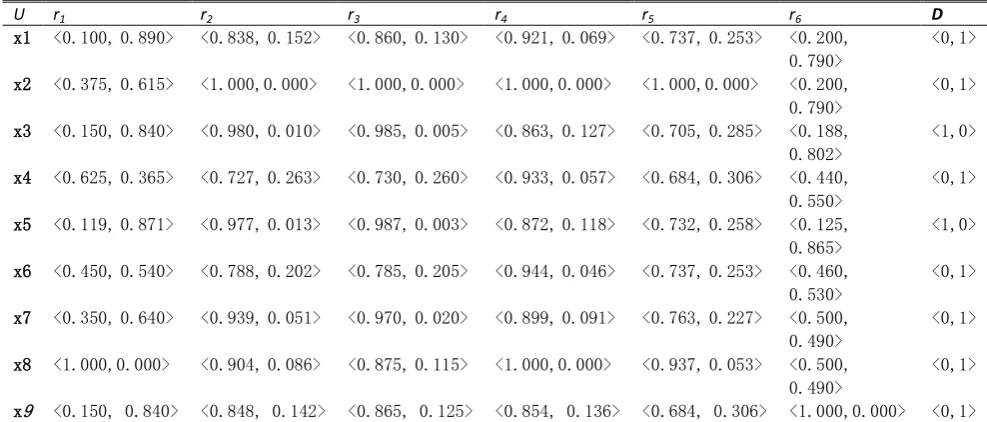
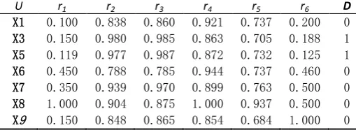
x1 0.100 0.838 0.860 0.921 0.737 0.200 0 x2 0.375 1.000 1.000 1.000 1.000 0.200 0 x3 0.150 0.980 0.985 0.863 0.705 0.188 1 x4 0.625 0.727 0.730 0.933 0.684 0.440 0 x5 0.119 0.977 0.987 0.872 0.732 0.125 1 x6 0.450 0.788 0.785 0.944 0.737 0.460 0 x7 0.350 0.939 0.970 0.899 0.763 0.500 0 x8 1.000 0.904 0.875 1.000 0.937 0.500 0 x9 0.150 0.848 0.865 0.854 0.684 1.000 0

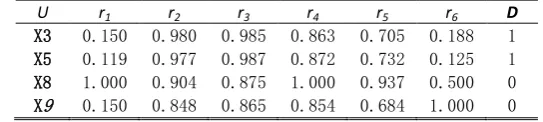
The intuitionistic fuzzy similarity relation

S P

( )

(which the matrix is symmetric) of the table is obtained,

U r1 r2 r3 r4 r5 r6 D

x1 <0.100,0.890> <0.838,0.152> <0.860,0.130> <0.921,0.069> <0.737,0.253> <0.200, 0.790>

<0,1>

x2 <0.375,0.615> <1.000,0.000> <1.000,0.000> <1.000,0.000> <1.000,0.000> <0.200, 0.790>

<0,1>

x3 <0.150,0.840> <0.980,0.010> <0.985,0.005> <0.863,0.127> <0.705,0.285> <0.188, 0.802>

<1,0>

x4 <0.625,0.365> <0.727,0.263> <0.730,0.260> <0.933,0.057> <0.684,0.306> <0.440, 0.550>

<0,1>

x5 <0.119,0.871> <0.977,0.013> <0.987,0.003> <0.872,0.118> <0.732,0.258> <0.125, 0.865>

<1,0>

x6 <0.450,0.540> <0.788,0.202> <0.785,0.205> <0.944,0.046> <0.737,0.253> <0.460, 0.530>

<0,1>

x7 <0.350,0.640> <0.939,0.051> <0.970,0.020> <0.899,0.091> <0.763,0.227> <0.500, 0.490>

<0,1>

x8 <1.000,0.000> <0.904,0.086> <0.875,0.115> <1.000,0.000> <0.937,0.053> <0.500, 0.490>

<0,1>

(16)

1 0.100 1 0.100 0.150 1 0.100 0.200 0.150 1 0.100 0.119 0.119 0.119 1 0.100 0.200 0.150 0.440 0.119 1 0.100 0.200 0.150 0.350 0.119 0.350 1 0.100 0.200 0.150 0.440 0.119 0.450 0.350 1 0.100 0.150 0.150 0.150 0.119 0.150 0.150 0.150 1 ( )= S P                            

 

xQ=



x x x x x x x1, 2, 4, 6, 7, 8, 9

 

, x x3, 5



, let

 

xQ=



A B,



,it is obtained,

  





























 

1 2 4 6 7 8 9 0.900, 0 , ,

0.800, 0.100 , ,

0.560, 0.034 , ,

0.550, 0.350 , , ( )

0.650, 0.250 , ,

0.500, 0.400 , ,

0.850, 0.050 , ,

0,1 , i x x x x x x x x

S P A x

x x x x x x others       _   _        _      ；

  









 

3 5

0.850, 0.050 , ,

( ) 0.881, 0.019 , ,

0,1 ,

i

x x

S P B x x x

others     _    ；

The discernibility matrix M U PQ( , ) is calculated,as

1 1 1 1

1 1

1 6 1 1 1 1 1

1 6 1 6 1 1 1 1 6 1 1 1 1 6 1 6 1 1 1 1

1 1

( , )=

Q

r r r r

r r

r r r r r r

r

r r r r r r r

r r r r r

r r r r r r r r

r r

M U P

                                                                        

The weights of attributes in the intuitionistic fuzzy rough discernibility matrix are calculated,

1 2 3 4 5 6

( ) 251, ( ) 0, ( ) 0, ( ) 0, ( ) 0, ( ) 54

W r  W r  W r  W r  W r  W r 

1 2 3 4 5 6

( ) 29, ( ) 0, ( ) 0, ( ) 0, ( ) 0, ( ) 6

Card r  Card r  Card r  Card r  Card r  Card r 

After the first round of calculation, Red (P) =

{ }

r

₁ , the combinations of attribute

r

₁ in the discernibility

matrix are set as emptied, and the weights of all the attributes are calculated.

1 2 3 4 5 6

( ) 0, ( ) 0, ( ) 0, ( ) 0, ( ) 0, ( ) 54

W r  W r  W r  W r  W r  W r 

1 2 3 4 5 6

( ) 0, ( ) 0, ( ) 0, ( ) 0, ( ) 0, ( ) 6

After the second round of calculation, Red (P) =

{ , }

r r

1 6 , and the combinations of attribute

r

6 in the

(17)

1 2 3 4 5 6

( ) 0, ( ) 0, ( ) 0, ( ) 0, ( ) 0, ( ) 0

W r  W r  W r  W r  W r  W r 

1 2 3 4 5 6

( ) 0, ( ) 0, ( ) 0, ( ) 0, ( ) 0, ( ) 0

The final reduction is Red (P)=

{ , }

r r

₁ ₆ .

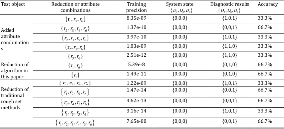
5.2. Sampling and Reduction

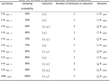
Two subgroups which are containing90%、80%、70%、60%、50% samples were extracted respectively from original decision information system, and they are noted as F-R（90%，1）、F-R（90%，2）、F-R（80%，1）、F-R（80%，

2）、F-R（70%，1）、F-R（70%，2）、F-R（60%，1）、F-R（60%，2）、F-R（50%，1）、F-R（50%，2）,Seen in Tab. 3~12.Their reductions

are noted as R（90%，1）、R（90%，2）、R（80%，1）、R（80%，2）、R（70%，1）、R（70%，2）、R（60%，1）、R（60%，2）、R（50%，1）、R

（50%，2）.

Table 3. Sampled Intuitionistic Fuzziness Sub-decision Information System（F-R（90%, 1））

U r1 r2 r3 r4 r5 r6 D

X1 0.100 0.838 0.860 0.921 0.737 0.200 0 X2 0.375 1.000 1.000 1.000 1.000 0.200 0 X3 0.150 0.980 0.985 0.863 0.705 0.188 1 X4 0.625 0.727 0.730 0.933 0.684 0.440 0 X5 0.119 0.977 0.987 0.872 0.732 0.125 1 X7 0.350 0.939 0.970 0.899 0.763 0.500 0 X8 1.000 0.904 0.875 1.000 0.937 0.500 0 X9 0.150 0.848 0.865 0.854 0.684 1.000 0

U r1 r2 r3 r4 r5 r6 D

X1 0.100 0.838 0.860 0.921 0.737 0.200 0 X3 0.150 0.980 0.985 0.863 0.705 0.188 1 X4 0.625 0.727 0.730 0.933 0.684 0.440 0 X5 0.119 0.977 0.987 0.872 0.732 0.125 1 X6 0.450 0.788 0.785 0.944 0.737 0.460 0 X7 0.350 0.939 0.970 0.899 0.763 0.500 0 X8 1.000 0.904 0.875 1.000 0.937 0.500 0 X9 0.150 0.848 0.865 0.854 0.684 1.000 0

U r1 r2 r3 r4 r5 r6 D

X1 0.100 0.838 0.860 0.921 0.737 0.200 0 X2 0.375 1.000 1.000 1.000 1.000 0.200 0 X3 0.150 0.980 0.985 0.863 0.705 0.188 1 X4 0.625 0.727 0.730 0.933 0.684 0.440 0 X5 0.119 0.977 0.987 0.872 0.732 0.125 1 X8 1.000 0.904 0.875 1.000 0.937 0.500 0 X9 0.150 0.848 0.865 0.854 0.684 1.000 0

U r1 r2 r3 r4 r5 r6 D