Numerical Study On Natural Convection In A Rectangular Cavity With Partially Active Side Walls

(1)

Page 319 www.ijiras.com | Email: [email protected]

Numerical Study On Natural Convection In A Rectangular Cavity

With Partially Active Side Walls

K. Gayathri Devi

Research Scholar, Department of Mathematics, Sri Krishnadevaraya University, Anantapuramu, A.P., India

R. Siva Prasad

Professor, Department of Mathematics,

Sri Krishnadevaraya University, Anantapuramu, A.P., India

I. INTRODUCTION

A natural convection flow in a rectangular cavity has many engineering and geo-physical applications with different heating locations. In the fields like solar energy collection and cooling of electronic components, the active walls may be subject to abrupt temperature non-uniformities due to shading or other effects. With a view to understand the above problem, we shall first look into the studies related to the above problem. The effect of aspect ratio on flow structure and the convective heat transfer in a rectangular porous cavity is numerically analyzed by Prasad and Kulacki [1] Multicellular flow has been found for Ar ≤ 1 and the flow structure comprises a primary recirculating cell with smaller secondary cells inside. Paolucci and Chenoweth [2] studied the natural convection in shallow enclosures with differentially heated end walls. They find that the classical parallel flow solution, accurate in the core of the cavity in the Boussinesq limit, does not exist when variable properties are introduced.

Ho and Chang [3] numerically and experimentally studied the effect of aspect ratio of natural convection heat transfer in a vertical rectangular enclosure with two-dimensional discrete heating. Numerical simulation is conducted for aspect ratio varying from 1 to 10 with given relative heater size and location. From the numerical simulation, they find that the

effect of enclosure aspect ratio on the average Nusselt number of the discrete heaters tends to decrease with the increase of the modified Rayleigh number. R.L. Frederick [4] concludes the Nusselt number decreases rapidly with increasing aspect ratio and the circulation rate increases always with the Rayleigh number and with aspect ratio by the investigation of a numerical study of natural convection of air in rectangular cavities. Wakitani [6] numerically presented the three dimensional oscillatory natural convection at low Prandtl number in rectangular enclosures. His numerical results agreed with available experimental results.

The effect of the surface waviness and aspect ratio on heat transfer inside a wavy enclosure is studied numerically by Das et al. [7]. It shows that the heat transfer is changed considerably when the surface waviness changes and also depends on the aspect ratio of the domain. Effect of the aspect ratio of thermal–fluid transport phenomena in cavities under reduced gravity is studied numerically by Torii [8]. Valencia and R.L.Frederick [9] have investigated the natural convection of air in a square cavity with partially active vertical walls for five different heating locations. The heat transfer rate is enhanced when heating location is at the middle of the hot wall. El-Refaee et al. [10] have studied numerically natural convection in a partially cooled, differentially heated tilted cavities with different aspect ratios. Deng et al. [11] have

Abstract: In this paper, we examine the effect of natural convection in a rectangular cavity with partially active side walls for different heating locations i.e. for the hot region located at the top, middle and bottom, the cold region moved from bottom to top where the heat transfer rate is maximum and minimum. The Galerkin Finite Element Method has been used to convert the Partial Differential Equations into matrix form of equations and dividing the physical domain into smaller segments, which is a pre-requisite for Finite Element Method. Numerical results are presented in terms of stream functions and isotherms, which shows the effect of the aspect ratio with different heating locations.

(2)

Page 320 www.ijiras.com | Email: [email protected] investigated a combined temperature scale for analyzing

natural convection in a rectangular enclosure with discrete wall heat sources. They conclude that the role of isothermal heat sources is generally much stronger than the flux of heat sources.Nithyadevi et al. [12] studied natural convection in a square cavity with partially active vertical walls. Kandaswamy et al. [13] investigated maximum density effects of water in a square cavity with partial thermally active side walls.

In view of these, we studied a natural convection in a rectangular cavity with partially active side walls for different heating locations. That is, for the hot region located at the top, middle and bottom and the cold region moved from bottom to top, to locate the regions where the heat transfer rate is maximum and minimum. The Galerkin Finite Element Method has been used to convert the partial differential equations into a matrix form of equations, which can be solved iteratively with the help of a computer code. A three nodded triangular elements is used to divide the physical domain into smaller segments, which is a pre-requisite for finite element method. Numerical results are presented in terms of stream functions and isotherms, which shows the effect of the aspect ratio with different heating locations of the side walls. The mid-height velocity profile of the middle-middle heating locations for different aspect ratios Ar = 1, 3, 5, 10 and Gr = 105 are discussed.

II. MATHEMATICAL FORMULATION

We consider the laminar convective flow of a fluid in a rectangular cavity of length L and height H filled with a fluid under investigation. The partially thermally active side walls of the cavity are maintained at two different but uniform temperatures, namely,

T

_h and

T

_C (

T

_h >

T

_C), respectively. The inactive parts of the side walls and horizontal walls x = 0 and x = H are thermally insulated. For different heart regions will be studied here. That is, for the hot region located at the top, middle and bottom, assume a cold region moved from bottom to top. The length of the thermally active part is H/2. Representing the position through Cartesian coordinate system and assuming all other fluid properties to be constant, the flow of an incompressible Boussinesq viscous fluid.

Under the above specified geometrical and physical conditions is governed by the momentum and energy can be written as



























2 2

y

T

x

T

y

T

v

x

T

u



(2.3)

With boundary conditions

t=0: u = v = 0, T = Tc,

0 

x



H

,

0 

y



L

,

t > 0: u = v = 0,

0 ,

x

0 and

H

,

x

T

_



T = Th, on the hot part, y = 0,

T = Tc, on the cold part, y = L,

0 ,

y

0 and

L

,

y

T





The Continuity equation (2.1) can be satisfied automatically by introducing the stream function ‘’ as

u =

y





and v =

x







(2.4)

where x and y are the distances measured along the horizontal and vertical directions, respectively; r and z are the velocity components in the x- and y- directions, respectively; T denotes the temperature; and



are kinematic viscosity and thermal diffusivity, respectively; K is the medium permeability; P is the pressure and is the density; Th and Tc

are the temperatures at hot bottom wall and cold vertical walls, respectively; L is the side of the square cavity.

Using the following change of variables,

. ,

,

, ,

2 2

c h

c

T T

T T L

y Y H

x X

L v

v V L vH

u U HL v v

v L

t

   



 



   

 

The governing equations (2.1)-(2.3) reduce to non-dimensional form and introducing stream function

0 







Y

V

X

U

(2.5)

Y Ar Gr Y X Ar Y X X

Y 

                  

       

 

2 2 2 2 2 1

(2.6)































2 2

2

1 Pr

1 Y

X

Ar

Y

X

Y













(2.7) With the non dimensionless boundary conditions are

,

1

0 ,

1

0 ,

0 :

0 











X

Y



1

0 ,

0 :

0 at

X

and

X

Y





















,

.

1

0 ,

0

0 ,

1 ,

0 ,

1 ,

0 and

Y

at

Y

at

part

cold

the

on

X

Y

at

part

hot

the

on

Y



























(3)

Page 321 www.ijiras.com | Email: [email protected] III. SOLUTION OF THE GOVERNING EQUATIONS

Thus far we have derived the partial differential equations, which describe the heat and fluid flow behavior in the vicinity of porous medium. The development of governing equations is one part but the second and important part is to solve these equations in order to predict the various parameters of interest in the porous medium. There are various numerical methods available to achieve the solution of these equations, but the most popular numerical methods are Finite difference method, Finite volume method and the Finite element method. The selection of these numerical methods is an important decision, which is influenced by variety of factors amongst which the geometry of domain plays a vital role. Other factors include the ease with which these partial differential equations can be transformed into simple forms, the computational time required and the flexibility in development of computer code to solve these equations.

In the present study, we have predominantly used Finite Element Method (FEM) except for one case in which Finite difference method was utilized, as it was particularly suitable for that case. The following sections enlighten the Finite element method and present its application to solve the above-mentioned equations.

The Finite Element Method is a deservingly popular method amongst scientific community. This method was originally developed to study the mechanical stresses in a complex airframe structure popularized by Zienkiewicz and Cheung (23) by applying it to continuum mechanics. Since then the application of Finite Element Method has been exploited to solve the numerous problems in various engineering disciplines. The great thing about finite element method is its ease with which it can be generalized to myriad engineering problems comprised of different materials.

Another admirable feature of the Finite Element Method (FEM) is that it can be applied wide range of geometries having irregular boundaries, which is highly difficult to achieve with other contemporary methods. FEM can be said to have comprised of roughly 5 steps to solve any particular problem. The steps can be summarized as

 Descritizing the domain: This step involves the division of whole physical domain into smaller segments known as elements, and then identifying the nodes, coordinates of each node and ensuring proper connectivity between the nodes.

 Specifying the equation: In this step, the governing equation is specified and an equation is written in terms of nodal values

 Development of Global matrix: The equations are arranged in a global matrix which takes into account the whole domain

 Solution: The equations are solved to get the desired variable at each table in the domain

 Evaluate the quantities of interest: After solving the equations a set of values is obtained for each node, which can be further processed to get the quantities of interest. There are varieties of elements available in FEM, which are distinguished by the presence of number of nodes. The present study is carried out by using a simple 3-noded triangular element.

Let us consider that the variable to be determined in the triangular area is ‘



’. The polynomial function for ‘



’ can be expressed as:



= 1 + 2x + 3y (1)

The variable



has the value



i,



j and



k at the nodal

position i, j, and k of the element. The x and y coordinates at these points are xi, xj, xk and yi, yj and yk respectively.

Substitution of these nodal values in the equation (1) helps in determining the constants 1 , 2 , 3 which are:

1 = 1/2A [(xj yk – xk yj )



i + (xk yi – xi yk)



j + (xi yj – xj

yi)



k ]

2 = 1/2A [(yj - yk )



i + (yk – yi )



j + (yi – yj )



k ]

3 = 1/2A [(xk - xj )



i + (xi – xk )



j + (xj – xi )



k ]

where A is area of the triangle given as

k k

j j

i i

y

x

y

x

y

x

A

1

2 

Substitution of 1, 2, 3 in the equation (1) and

mathematical arrangement of the terms results into



= Ni



i + Nj



j + Nk



k

In equation (6), Ni, Njand Nk are the shape function given

by

A

y

c

x

b

a

N

_m m m m

2 





, m = i, j, k

The constants can be expressed in terms of coordinates as ai = xj yk – xk yj

bi = yj – yk

ci = xk - xj

aj = xk yi – xi yk

bj = yk – yi

cj = xi – xk

ak = xi yj – xj yi

bk = yi - yj

ck = xj – xi

The triangular element can be subdivided into three triangles with a point in the center of original triangle.

Defining the new area ratios as

ijk

area

pij

area

L

1



ijk

area

pjk

area

L

2



ijk

area

pki

area

L

3



It can be shown that L1 = N1

L

₂ = N2

L

₃ = N3

(4)

Page 322 www.ijiras.com | Email: [email protected] equations into matrix form for an element. The steps invented

are as given below.

Please note that the nodal terms i, j & k are replaced by 1,2 & 3 respectively in subsequent discussions for simplicity.

The momentum and energy balance equations are solved using the Galerkin finite element method. Continuity equation will be used as a constraint due to mass conservation and this constraint may be used to obtain the pressure distribution. In order to solve equations, we use the finite element method where the pressure P is eliminated by a penalty parameter



and the incompressibility criteria given by equation (2.1) which results in























Y

z

X

r

P



*

The continuity equation (2.5) is automatically satisfied for large values of



.

Application of Galerkin method to equation (2.6) yields:

 

dXdY

Y Ar Gr Y X Ar Y X X Y N R A T e                              _          2 2 2 2 2 1 (2.8)

Where Re is the residue.

Considering the terms individually



, ,



4

1 ]

[ ₁ ₂ ₃

3 3 2 2 1 1 3 3 2 2 1 1 3 3 2 2 1 1 b b b c c c c c c c c c A dA X Y N A T                     



         

 (2.9)



, ,



12

1 ]

[ 1 2 3

3 3 2 2 1 1 3 3 2 2 1 1 3 3 2 2 1 1 c c c b b b b b b b b b A dA Y X N A T                     



           (2.10) 12 1 1 ] [ 3 2 1 2 3 3 2 3 1 3 2 2 2 2 1 3 1 2 1 2 1 2 2 2 2                       



    b b b b b b b b b b b b b b b Ar A dA X Ar N A T (2.11)

































3 2 1 2 3 3 2 3 1 3 2 2 2 2 1 3 1 2 1 2 1 2 2

4

1 ]

[





c

A

dA

Y

N

A T But

 

dA

Y

N

L

Gr

dA

Y

Ar

Gr

N

A A T





_





_



_





_





_





























_

3 2 1

Pr

]

[



1 1 2 2 3 3



1

12

1 Pr

c



c



c



A

Gr

















(2.12)

Thus the whole equation (2.8) can be written in matrix form as













0

1 1 1 12 1 Pr 4 1 12 1 , , 12 1 , , 4 1 3 3 2 2 1 1 3 2 1 2 3 3 2 3 1 3 2 2 2 2 1 3 1 2 1 2 1 3 2 1 2 3 3 2 3 1 3 2 2 2 2 1 3 1 2 1 2 1 2 3 2 1 3 3 2 2 1 1 3 3 2 2 1 1 3 3 2 2 1 1 3 2 1 3 3 2 2 1 1 3 3 2 2 1 1 3 3 2 2 1 1                                                                                                                     c c c A Gr c c c c c c c c c c c c c c c A b b b b b b b b b b b b b b b Ar A c c c b b b b b b b b b A b b b c c c c c c c c c A (2.13) FEM of Energy Equation

 

1 (2.14)

Pr 1 ] [ ₂ 2 2 2 2



_ _                          A T e dA Y X Ar Y X X Y N

R      

 

Considering the terms individually

 , ,  (2.15)

12 1 ] [ 3 2 1 3 2 1 3 3 2 2 1 1 3 3 2 2 1 1 3 3 2 2 1 1                                               b b b c c c c c c c c c A dA X Y N A T

 , ,  (2.16)

12 1 ] [ 3 2 1 3 2 1 3 3 2 2 1 1 3 3 2 2 1 1 3 3 2 2 1 1                                               c c c b b b b b b b b b A dA Y X NT A (2.17) 4 1 1 Pr 1 1 Pr 1 ] [ 3 2 1 2 3 3 2 3 1 3 2 2 2 2 1 3 1 2 1 2 1 2 2 2 2                              b b b b b b b b b b b b b b b A Ar dA X Ar N A T (2.18) 4 1 1 Pr 1 1 Pr 1 ] [ 3 2 1 2 3 3 2 3 1 3 2 2 2 2 1 3 1 2 1 2 1 2 2 2 2                              c c c c c c c c c c c c c c c A Ar dA Y Ar N A T

Thus the whole equation (2.14) can be written in matrix form as









(2.19) 0 4 1 1 Pr 1 4 1 1 Pr 1 , , 12 1 , , 12 1 3 2 1 2 3 3 2 3 1 3 2 2 2 2 1 3 1 2 1 2 1 2 3 2 1 2 3 3 2 3 1 3 2 2 2 2 1 3 1 2 1 2 1 2 3 2 1 3 2 1 3 3 2 2 1 1 3 3 2 2 1 1 3 3 2 2 1 1 3 2 1 3 2 1 3 3 2 2 1 1 3 3 2 2 1 1 3 3 2 2 1 1                                                                                                                               c c c c c c c c c c c c c c c A Ar b b b b b b b b b b b b b b b A Ar c c c b b b b b b b b b A b b b c c c c c c c c c A

IV. NUSSELT NUMBER

The ratio of the conductive thermal resistance to the convective thermal resistance of the fluid is called Nusselt number. This is writeen as Nu = hL/ K.

V. RESULTS AND DISCUSSIONS

The numerical solutions are found for different grid systems from 21



21 to 101



101. After 41



41 grids, no considerable change in the average Nusselt number is observed and hence a 41



41 grid is used in this study.

(5)

Page 323 www.ijiras.com | Email: [email protected] the bottom thermally active location. The flow is in two cells

and centers of the cells are located near the thermally active parts of the side walls. When compared to other positions the heat transfer rate is much less in this to wards conduction at the central region and convection near the active locations. As the cold wall is moved to the bottom, the isotherms predict almost conduction at the middle of the cavity. In this case, the circulation rate and velocity are very low compared to all the other cases.

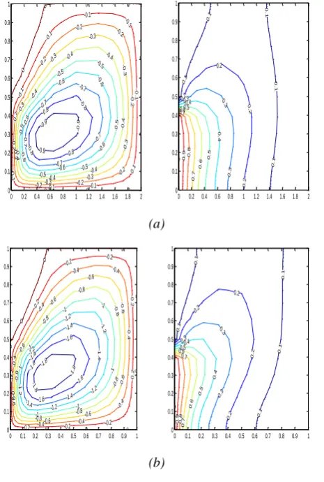
Fig. 2 shows that the middle–middle heating location, there is a strong thermal boundary layers are formed at the active locations and the existence of convection near the active locations is seen from the isotherms for aspect ratios 0.5, 1, 2, 3 and 5 and Gr = 105. The circulation rate and the heat transfer rate are maximum in this case compared to all the other cases. A single cell pattern is observed.

For the case of square cavity, there exist two inner cells each at the top left and bottom right corners of the cavity. The remaining two corners are less activated but this type of behaviour does not exist in the case of rectangular cavities. The two inner cells are moved to upper and lower parts of the cavity when Ar = 2. This is due to the dominating buoyancy force inside the cavity.

Further increasing the aspect ratio, the two inner cells grow in size and strength, while two small recirculating eddies occur in the middle of the cavity. Increasing the aspect ratio to 5 the recirculating zones in the middle of the cavity disappear. The isotherms for the middle–middle thermally active location, different aspect ratios and Gr = 105 are presented in Fig. 3.

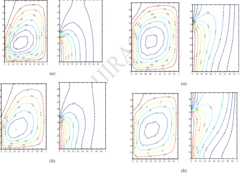
For all the aspect ratios, a thermal boundary layer exists along the active zones. Large velocity and temperature gradients characterize the region immediately adjacent to the thermally active side wall locations while negligible gradients (normal to the hot/cold wall location) prevail in the rest of the cavity. Such behaviour is indicative of the thermal boundary layer structure. Fig. 3 shows the flow pattern for the middle– bottom heating location, different aspect ratios and Gr = 105.

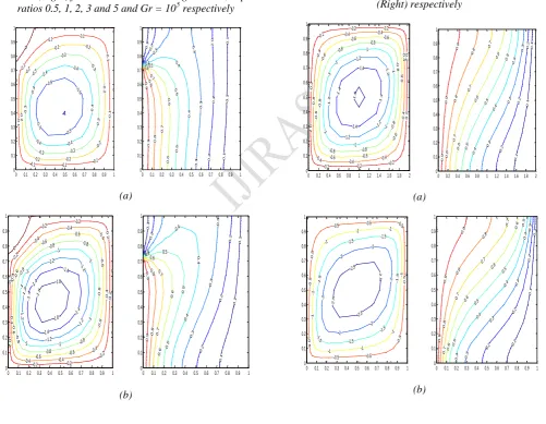
In the case of square cavity, the two inner cells exist in the middle left and bottom right active parts of the cavity. On increasing the aspect ratio, the two inner cells disappear and the major cell is skewed upward along the hot wall and downward along the cold wall. Further on increasing the aspect ratio, upper part of the cavity remains stagnant while the lower part of the cavity is more activated. A secondary cell exists within the primary cell in the lower part of the cavity. With increase in the aspect ratio of the cavity, the buoyant convection flow is increasingly strengthened. The isotherms for the middle– bottom thermally active location, for different aspect ratios are displayed in Fig. 3. The same behaviour is observed as in Fig. 2. Figures 4., and Fig. 5., shows the streamlines and isotherms for Grashof numbers top , middle and bottom heating locations for Ar = 3 and for Gr = 103. There exists a clockwise rotating cell in the middle portion of the cavity. The fluid in the upper and lower parts of the cavity is stagnant.

When Gr = 104 and Ar = 3, the circulation rate of the eddy is increased and the unicellular pattern is enlarged and occupies the whole cavity. Further increasing Gr = 105 and Ar = 3, there exist a unicellular pattern. The velocity of the fluid

particle inside the cavity and also the buoyant convection flow increases by increasing the Grashof number.

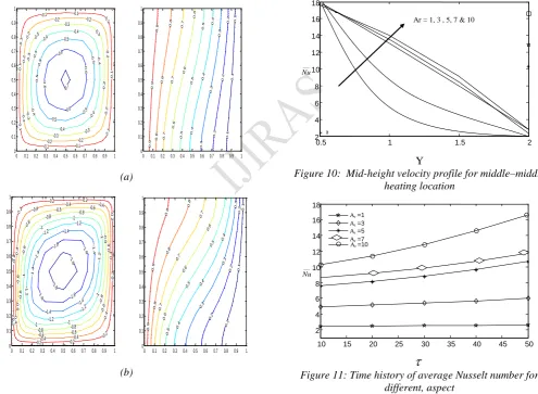
Fig. 7 shows the mid-height velocity profile for different aspect ratios and middle–middle heating locations for Gr = 105 and for different aspect ratios. The increase in the vertical velocity of the fluid particles at mid-height of the cavity for increasing aspect ratio near the active locations is shown.

The time history of the average Nusselt number for different aspect ratios and Gr = 105 at middle–middle heating locations are displayed in Fig. 8. Thus the average Nusselt number is increased as the aspect ratio increases. Increasing the aspect ratio increases the time to reach the steady state situation of the solution.

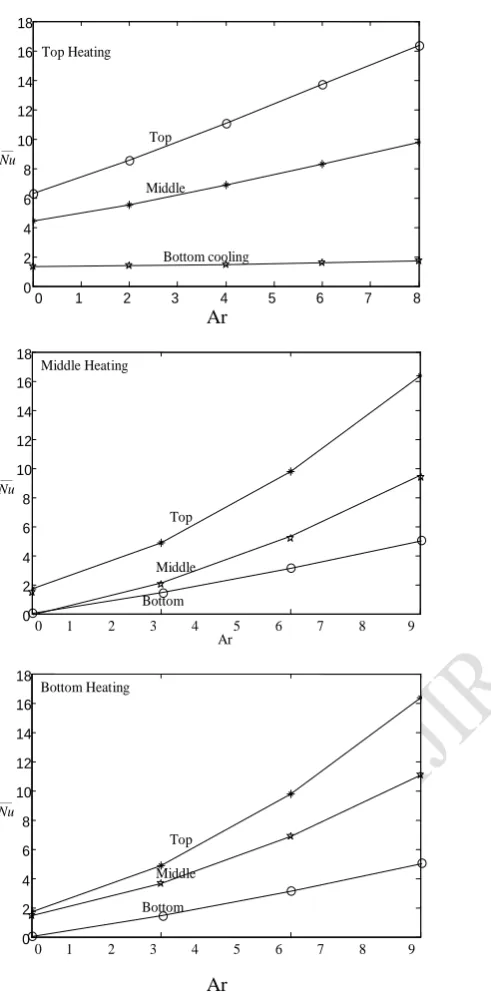
Average Nusselt number for different aspect ratios, different Grashof numbers for different heating locations ( top, middle and bottom heating ) is depicted in Fig. 9. The heat transfer rate is increased by increasing both the aspect ratio and the Grashof number.

In order to evaluate how the aspect ratio and different heating locations affects the heat transfer rate, the average Nusselt number is plotted as a function of aspect ratio for different thermally active zones in Fig. 9.

Heat transfer rate is increased on increasing the aspect ratio. There is no considerable variation in the average Nusselt number for Ar



1 when the heating/cooling locations are changed. The heat transfer rate is enhanced when a cooling location is at the top of the enclosure. When changing the heating location from top to bottom the average Nusselt number is increased by increasing the aspect ratio. It is clearly seen from Fig. 9.

-0.9

-0 .8 _-0.8

-0 .8 -0.8

-0

.

7

-0.7 -0.7 -0.7

-0.7

-0 .6

-0.6

-0 .6

-0.6

-0 .6

-0.5

-0.5 -0.5

-0.5 -0.5 -0.5

-0

.4

-0.4

-0 .4

-0.4

-0

.3

-0.3 -0.3

-0 .3

-0.3

-0

.

2

-0.2 -0.2

-0.2

-0

.2

-0.2

-0 .2

-0

.1

-0.1 -0.1

-0.1

-0

.1

-0_.1

-0.1

-0 .1

0

0 0 0

0

0 0

0

0 0.2 0.4 0.6 0.8 1 1.2 1.4 1.6 1.8 2 0

0.1 0.2 0.3 0.4 0.5 0.6 0.7 0.8 0.9 1

0.1

0

.

1

0

.

1

0. 1

0.

2

0

.

2

0.2

0. 3 0_.3

0.3

0

.

4

0.4

0.

5

0.5

0

.6

0.6

0.

7

0.7

0

.

8

0.

9

1

0 0.2 0.4 0.6 0.8 1 1.2 1.4 1.6 1.8 2 0

0.1 0.2 0.3 0.4 0.5 0.6 0.7 0.8 0.9 1

(a)

-1 .8

-1.8

-1.6

-1.6 -1.6

-1.6

-1.4 -1.4

-1

.4

-1.4

-1

.2

-1.2 -1.2

-1 .2

-1.2

-1

-1 -1 -1 -1

-1

-0

.8

-0.8 -0.8

-0 .8 -0

.8 -0.8

-0.8

-0

.6

-0.6 -0.6

-0 .6

-0 .6 -0.6

-0.6

-0

.

4

-0.4 -0.4

-0.4

-0

.4

-0.4 -0.4

-0.4

-0

.2

-0.2 -0.2 -0.2

-0

.2

-0

.2

-0.2

-0 .2

0

0 0 0

0

0 0

0

0 0.1 0.2 0.3 0.4 0.5 0.6 0.7 0.8 0.9 1 0

0.1 0.2 0.3 0.4 0.5 0.6 0.7 0.8 0.9 1

0.

1

0.1

0.1 0. 1

0

.

1

0.2

0.

2

0.2

0.3 0.3

0.3

0.4

0.5

0.6

0.

7

0.7

0

.

8

0.

9

1

0 0.1 0.2 0.3 0.4 0.5 0.6 0.7 0.8 0.9 1 0

0.1 0.2 0.3 0.4 0.5 0.6 0.7 0.8 0.9 1

(6)

-3.5

-3 _-3

-3

-2_.5 -2.5

-2.5 -2.5

-2.5

-2

-1

.5

-1.5

-1.5 -1.5

-1

.5

-1.5

-1

-1 -1

-1

-0.5 -0.5 -0.5

-0

.5

-0

.5

-0.5

-0

.5

0

0 0 0

0

0 0

0

0.5

0 0.05 0.1 0.15 0.2 0.25 0.3 0.35 0.4 0.45 0.5 0

0.1 0.2 0.3 0.4 0.5 0.6 0.7 0.8 0.9 1

0

.

1

0

.1

0.1

0

.

1

0

.

2

0.2

0.2 0.2

0.

2

0.3 0.3

0

.

3

0.3

0.4 0.4

0.4

0 .5

0.5

0.6

0. 7

0.7

0

.

8

0.8

0

.

9

1

0 0.05 0.1 0.15 0.2 0.25 0.3 0.35 0.4 0.45 0.5 0

0.1 0.2 0.3 0.4 0.5 0.6 0.7 0.8 0.9 1

(c)

Figure 1: Stream functions (Left) for all heating locations, Ar

= 2 and Gr = 105 and Isotherms (Right) for all heating

locations, Ar = 2 and Gr = 105 respectively

-0.35

-0

.3

5

-0.35

-0.3

-0.25 -0.25

-0 .2 5

-0.25

-0

.2

-0.2 -0.2

-0

.2

-0.2

-0.15 _-0.15 -0.15

-0

.1

5

-0.15

-0.1 5

-0

.1

-0.1 -0.1

-0.1

-0

.1

-0.1

-0

.0

5

-0.05 -0.05 -0.05

-0

.0

5

-0 .0 5

-0.05

-0.0 5

0

0 0 0

0

0 0

0

0 0.1 0.2 0.3 0.4 0.5 0.6 0.7 0.8 0.9 1 0

0.1 0.2 0.3 0.4 0.5 0.6 0.7 0.8 0.9 1

0.1

0 .1

0

.

1

0

.

2

0.2 0.2

0

.

3

0.3

0

.4 0.4

0

.

5

0.5

0

.

6

0.6

0.

7

0.7 0 .8

0

.

9

1

0 0.1 0.2 0.3 0.4 0.5 0.6 0.7 0.8 0.9 1 0

0.1 0.2 0.3 0.4 0.5 0.6 0.7 0.8 0.9 1

(a)

-1

-1 -1

-0

.8

-0.8

-0.8 -0.8

-0 .6

-0.6 -0.6

-0 .6 -0_.6 -0.6

-0.6

-0

.4

-0.4 -0.4

-0.4

-0

.4

-0.4

-0

.

2

-0.2 -0.2

-0.2

-0

.

2

-0 .2

-0.2

0

0 0 0

0

0 0

0

0 0.1 0.2 0.3 0.4 0.5 0.6 0.7 0.8 0.9 1 0

0.1 0.2 0.3 0.4 0.5 0.6 0.7 0.8 0.9 1

0.1

0

.

1

0

.

1

0. 1

0 .2

0

.

2

0.2

0.3

0 .3

0.3

0

.

4

0.4

0. 5

0.5

0 .6

0.6

0

.7

0.70 .8 0 .9

1

0 0.1 0.2 0.3 0.4 0.5 0.6 0.7 0.8 0.9 1 0

0.1 0.2 0.3 0.4 0.5 0.6 0.7 0.8 0.9 1

(b)

-1

.8 -1

.8 -1.8

-1 .6 -1.6

-1 .6

-1.6

-1 .4 _-1.4

-1 .4

-1.4

-1

.2

-1.2

-1 .2

-1.2

-1

-1 -1

-1

-0 .8 _-0.8

-0.8

-0

.8

-0.8

-0 .6

-0.6 -0.6

-0

.6 -0

.6 -0.6

-0.6

-0 .6

-0

.

4

-0.4 -0.4

-0.4

-0

.

4

-0.4 -0.4

-0.4

-0

.

2

-0.2 -0.2 -0.2

-0

.2

-0

.2

-0.2

0

0 0 0

0

0 0

0

0 0.1 0.2 0.3 0.4 0.5 0.6 0.7 0.8 0.9 1 0

0.1 0.2 0.3 0.4 0.5 0.6 0.7 0.8 0.9 1

0.

1

0.1

0.

1

0

.

1

0.2 0. 2

0.2

0.3 0

.

3

0.3

0

.

4

0.4

0.5

0. 6 0.6

0

.

7

0.7

0

.

8

0

.

9

1

0 0.1 0.2 0.3 0.4 0.5 0.6 0.7 0.8 0.9 1 0

0.1 0.2 0.3 0.4 0.5 0.6 0.7 0.8 0.9 1

(c)

Figure 2: Stream functions (Left) for middle–middle heating

location, aspect ratios 0.5, 1, 2, 3 and 5 and Gr = 105

Isotherms (Right) for middle–middle heating location, aspect

ratios 0.5, 1, 2, 3 and 5 and Gr = 105 respectively

-1.4

-1_.2

-1.2 -1

.2 -1.2

-1

-1 -0 .8

-0.8 -0.8

-0 .8 -0

.8 -0.8

-0.8

-0

.6

-0_.6 -0.6

-0.6

-0

.6

-0.6 -0.6

-0.6

-0

.4

-0 .4

-0.4 -0.4

-0 .4

-0

.4

-0.4

-0

.2

-0 .2

-0.2 -0.2

-0 .2

-0

.2

-0.2 -0.2

-0.2

0

0 0 0

0

0 0

0

0 0.2 0.4 0.6 0.8 1 1.2 1.4 1.6 1.8 2

0 0.1 0.2 0.3 0.4 0.5 0.6 0.7 0.8 0.9 1

0 .1

0. 1

0

.

1

0.

1

0.2

0.2 0.2

0.

2

0.3

0.3 0.3

0

.

3

0.4 0

.

4

0.4

0.5

0 .5

0.5

0. 6

0

.

6

0.6

0

.

7 0.7

0

.8 0.8

0

.

9

0 .9

1

0 0.2 0.4 0.6 0.8 1 1.2 1.4 1.6 1.8 2 0

0.1 0.2 0.3 0.4 0.5 0.6 0.7 0.8 0.9 1

(a)

-2 .5

-2.5 -2.5 -2

-2

-1

.5

-1.5 -1.5

-1

.5

-1.5 -1.5

-1 .5

-1

-1 -1 -1

-1

-0

.5

-0.5 -0.5 -0.5

-0

.5

-0

.5

-0.5

0

0 0 0

0

0 0

0

0 0.1 0.2 0.3 0.4 0.5 0.6 0.7 0.8 0.9 1 0

0.1 0.2 0.3 0.4 0.5 0.6 0.7 0.8 0.9 1

0

.

1

0.1

0 .1

0.

1

0.2

0.2 0.2

0

.

2 0.3

0.3

0.4 0.4

0.5 0.5

0.6 0.6

0.6

0

.7 0.7

0.7

0.

8

0

.

8

0

.9

0

.

9

1

0 0.1 0.2 0.3 0.4 0.5 0.6 0.7 0.8 0.9 1 0

0.1 0.2 0.3 0.4 0.5 0.6 0.7 0.8 0.9 1

(7)

Page 325 www.ijiras.com | Email: [email protected] -4.5 -4 -4 -4 -4 -4 -3 .5 -3.5 -3.5 -3 .5 -3.5 -3.5 -3 -3 -3 -3 -3 -3 -3 -2 .5 -2.5 -2.5 -2 .5 -2.5 -2.5 -2.5 -2 -2 -2 -2 -2 -2 -2 -2 -1 .5 -1.5 -1.5 -1.5 -1 .5 -1.5 -1.5 -1.5 -1 .5

-1 -1 -1

-1 -1 -1 -1 -1 -1 -0 .5

-0.5 -0.5 -0.5

-0 .5 -0 .5 -0.5 -0.5 -0.5 -0 .5 0 0

0 0 0

0 0 0 0 0 0 0.5 0 . 5

0 0.05 0.1 0.15 0.2 0.25 0.3 0.35 0.4 0.45 0.5 0 0.1 0.2 0.3 0.4 0.5 0.6 0.7 0.8 0.9 1 0 . 1 0.1 0.1 0 . 1 0 . 2 0.2 0.2 0.2 0 . 2 0.3 0.3 0.3 0.3 0. 3 0.4 0.4 0.4 0.4 0.4 0.5 0.5 0.5 0. 5 0.5 0. 6 0.6 0. 6 0.6 0. 7 0.7 0.7 0. 8 0 .8 0 . 9 0. 9 1 1

0 0.05 0.1 0.15 0.2 0.25 0.3 0.35 0.4 0.45 0.5 0 0.1 0.2 0.3 0.4 0.5 0.6 0.7 0.8 0.9 1 (c)

Figure 3: Stream functions (Left) for middle–bottom heating

location, aspect ratios 0.5, 1, 2, 3 and 5 and Gr = 105

Isotherms (Right) for middle–bottom heating location, aspect

ratios 0.5, 1, 2, 3 and 5 and Gr = 105 respectively

-0 .5 -0.5 -0_.5 -0.5 -0 .4 -0.4 -0.4 -0 .4 -0.4 -0.4 -0 .3 -0.3 -0.3 -0 .3 -0 .3 -0.3 -0.3 -0 .2 -0.2 -0.2 -0.2 -0 .2 -0.2 -0.2 -0.2 -0 .1

-0.1 -0.1 -0.1

-0 .1 -0 .1 -0.1 -0.1 -0.1 0 0

0 0 0

0 0 0 0 0 0

0 0.1 0.2 0.3 0.4 0.5 0.6 0.7 0.8 0.9 1 0 0.1 0.2 0.3 0.4 0.5 0.6 0.7 0.8 0.9 1 0. 1 0 . 1 0 . 1 0 . 1 0.2 0 . 2 0 . 2 0 .2 0.3 0 .3 0 . 3 0 .3 0 . 4 0.4 0.4 0. 5 0 .5 0.5 0 . 6 0 . 6 0.6 0 . 7 0.7 0 .8 0 .8 0 . 9 0 . 9 1 1

0 0.1 0.2 0.3 0.4 0.5 0.6 0.7 0.8 0.9 1 0 0.1 0.2 0.3 0.4 0.5 0.6 0.7 0.8 0.9 1 (a) -1 .6 -1.6 -1.6 -1.4 -1.4 -1.4 -1.4 -1.4 -1 .2 -1.2 -1.2 -1_.2 -1.2 -1 .2 -1 -1 _-1 -1 -1 -1 -1 -0 .8 -0.8 -0.8 -0 .8 -0.8 -0.8 -0.8 -0 .6 -0.6 -0.6 -0 .6 -0 .6 -0.6 -0.6 -0 .6 -0 . 4 -0.4 -0.4 -0.4 -0 .4 -0_.4 -0.4 -0.4 -0 .4 -0 .2 -0 .2 -0.2 -0.2 -0.2 -0 .2 -0 .2 -0.2 -0.2 -0.2 0 0

0 0 0

0 0 0 0 0 0

0 0.1 0.2 0.3 0.4 0.5 0.6 0.7 0.8 0.9 1 0 0.1 0.2 0.3 0.4 0.5 0.6 0.7 0.8 0.9 1 0 . 1 0. 1 0. 1 0 . 1 0.2 0.2 0.2 0 . 2 0.3 0.3 0.3 0. 3 0.4 0 . 4 0.4 0.4 0.5 0 .5 0.5 0. 6 0. 6 0.6 0. 7 0.7 0 . 8 0.8 0 . 9 0 .₉ 1 1

0 0.1 0.2 0.3 0.4 0.5 0.6 0.7 0.8 0.9 1 0 0.1 0.2 0.3 0.4 0.5 0.6 0.7 0.8 0.9 1 (b) -1.6 -1.6 -1.6 -1 .4 -1.4 -1.4 -1.4 -1.4 -1 .2 -1.2 -1.2 -1 .2 -1.2 -1 .2 -1 -1 _-1 -1 -1 -1 -1 -0 .8 -0.8 -0.8 -0 . 8 -0.8 -0.8 -0 .8 -0 .6 -0.6 -0.6 -0 .6 -0 .6 -0.6 -0.6 -0 .6 -0 . 4 -0.4 -0.4 -0.4 -0 .4 -0_.4 -0.4 -0.4 -0 .4 -0 .2 -0 .2 -0.2 -0.2 -0 .2 -0 .2 -0 .2 -0.2 -0.2 -0 .2 0 0

0 0 0

0 0 0 0 0 0

0 0.1 0.2 0.3 0.4 0.5 0.6 0.7 0.8 0.9 1 0 0.1 0.2 0.3 0.4 0.5 0.6 0.7 0.8 0.9 1 0. 1 0.1 0. 1 0 . 1 0 . 2 0.2 0.2 0 .2 0.3 0.3 0.3 0. 3 0.4 0.4 0. 4 0.4 0. 5 0.5 0 . 5 0.5 0. 6 0.6 0.6 0 . 7 0.7 0.7 0. 8 0.8 0 .9 0 . 9 1 1

0 0.1 0.2 0.3 0.4 0.5 0.6 0.7 0.8 0.9 1 0 0.1 0.2 0.3 0.4 0.5 0.6 0.7 0.8 0.9 1 (c)

Figure 4: Streamline Contour plots for Gr = 103 and Ar = 3.

Clockwise and anti-clockwise flows are shown via negative and positive signs of stream functions (Left) and Isotherms

(Right) respectively -1.6 -1 .4 -1.4 -1 .4 -1.4 -1 .2 -1.2 -1.2 -1 .2 -1.2 -1 -1 -1 -1 -1 -1 -1 -0 .8 -0.8 -0.8 -0 .8 -0 .8 -0.8 -0.8 -0 .6 -0.6 -0.6 -0.6 -0 .6 -0.6 -0.6 -0.6 -0 .4

-0.4 _-0.4 -0.4

-0 .4 -0 .4 -0.4 -0.4 -0 .4 -0 . 2

-0.2 -0.2 -0.2

-0 .2 -0 .2 -0.2 -0.2 -0.2 -0 .2 0 0 0

0 0 0

0 0 0 0 0 0

0 0.2 0.4 0.6 0.8 1 1.2 1.4 1.6 1.8 2 0 0.1 0.2 0.3 0.4 0.5 0.6 0.7 0.8 0.9 1 0.1 0 . 1 0 . 1 0.2 0.2 0. 2 0.3 0.3 0 .3 0.4 0.4 0.4 0.5 0.5 0.5 0.6 0.6 0.6 0 .7 0.7 0.7 0 . 8 0.8 0.8 0. 9 0 . 9 0 .9 1 1 1

0 0.2 0.4 0.6 0.8 1 1.2 1.4 1.6 1.8 2 0 0.1 0.2 0.3 0.4 0.5 0.6 0.7 0.8 0.9 1 (a) -2 .5 -2.5 -2 .5 -2.5 -2 -2 -2 -2 -2 -2 -1 .5 -1 .5 _-1.5 -1.5 -1 .5 -1.5 -1.5 -1 -1 -1 -1 -1 -1 -1 -1 -1 -0 .5 -0 .5 -0.5 -0.5 -0 .5 -0 .5 -0.5 -0.5 -0.5 -0 .5 0 0 0

0 0 0

0 0 0 0 0 0

0 0.1 0.2 0.3 0.4 0.5 0.6 0.7 0.8 0.9 1 0 0.1 0.2 0.3 0.4 0.5 0.6 0.7 0.8 0.9 1 0.1 0. 1 0 . 1 0.2 0.2 0. 2 0.3 0.3 0.3 0. 3 0 .4 0.4 0.4 0.4 0.5 0.5 0.5 0. 5 0. 6 0.6 0.6 0.6 0 .7 0.7 0.7 0.7 0 .8 0.8 0.8 0 . 9 0. 9 0.9 1 1 1

(8)

-4.5

-4

.5

-4.5

-4

-3

.5 -3.5

-3.5 -3 .5 -3.5

-3.5

-3

-3 -3

-3

-3 -3

-2

.5

-2.5

-2.5 -2.5

-2.5

-2 .5

-2

-2 -2

-2

-2 -2

-2

-1 .5

-1.5 -1.5

-1.5

-1

.5

-1.5 -1.5

-1.5

-1

.5

-1

-1 -1

-1

-1 -1

-1

-0

.5

-0 .5

-0.5 -0.5

-0 .5

-0

.5

-0

.5

-0.5 -0.5

-0 .5

0

0 0 0

0

0 0 0 0

0 0.05 0.1 0.15 0.2 0.25 0.3 0.35 0.4 0.45 0.5 0

0.1 0.2 0.3 0.4 0.5 0.6 0.7 0.8 0.9 1

0.1 0.1

0

.

1

0.2 0.2

0.2

0.

2

0.3 0.3

0.3 0. 3

0.4

0.4 0.4

0. 4

0.5

0.5 0.5

0.6 0.6

0

.

7

0.7 0.7

0.7

0

.

8

0.8 0.8

0.8

0

.

9

0.9 0.9

1

0 0.05 0.1 0.15 0.2 0.25 0.3 0.35 0.4 0.45 0.5 0

0.1 0.2 0.3 0.4 0.5 0.6 0.7 0.8 0.9 1

(c)

(Right) respectively

-0.7

-0

.6

-0.6

-0

.6

-0.6

-0

.5

-0.5 -0

.5 -0

.5

-0.5

-0 .5 -0

.4

-0 .4

-0.4

-0

.4

-0.4

-0 .3

-0.3 -0.3

-0

.3

-0_.3

-0.3

-0

.2

-0

.2

-0.2 -0.2

-0 .2

-0

.2

-0.2 -0.2

-0.2

-0

.1

-0

.1

-0.1 -0.1

-0 .1

-0

.1

-0 .1

-0.1 -0.1

-0

.1

0

0 0 0

0

0 0 0

0 0.1 0.2 0.3 0.4 0.5 0.6 0.7 0.8 0.9 1 0

0.1 0.2 0.3 0.4 0.5 0.6 0.7 0.8 0.9 1

0.

1

0

.1

0

.

1

0. 2 0 .2

0

.

2

0.

3

0. 3 0.

3

0 .4

0.4

0

.

4

0.

5

0 .5

0

.

5

0

.

6 0.6

0

.

6

0

.

7

0 .7

0.

8

0 .8 0.

8

0

.

9

0.

9

0

.9

1

0 0.1 0.2 0.3 0.4 0.5 0.6 0.7 0.8 0.9 1 0

0.1 0.2 0.3 0.4 0.5 0.6 0.7 0.8 0.9 1

(a)

-1_.8

-1 .8 -1

.6 _-1.6 -1

.6

-1.6

-1

.4

-1.4

-1

.4

-1.4

-1

.2

-1.2

-1

.2

-1.2

-1

-1 -1

-1

-0

.8

-0.8 -0.8

-0 .8

-0

.8

-0.8

-0 .8

-0

.6

-0.6 -0.6

-0 .6

-0

.6

-0.6 -0.6

-0.6

-0

.6

-0

.4

-0.4 -0.4

-0 .4

-0

.4

-0.4

-0

.4

-0

.2

-0

.2

-0.2 -0.2 -0

.2

-0

.2

-0

.2

-0.2 -0.2

-0.2

0

0 0 0

0

0 0 0

0 0.1 0.2 0.3 0.4 0.5 0.6 0.7 0.8 0.9 1 0

0.1 0.2 0.3 0.4 0.5 0.6 0.7 0.8 0.9 1

0.1

0

.1

0

.

1

0.2 0.2

0

.2

0.3

0

.

3

0.4

0.5 0.5

0.5

0.6

0.7 0.7

0.7

0 .8

0.8 0. 8

0

.

9

0. 9

0.9

1

0 0.1 0.2 0.3 0.4 0.5 0.6 0.7 0.8 0.9 1 0

0.1 0.2 0.3 0.4 0.5 0.6 0.7 0.8 0.9 1

(b)

-2.5

-2

-2 -2

-2

-1.5

-1 .5

-1.5

-1

.5

-1.5

-1

-1 -1

-1

-1 -1

-1

-0

.5

-0 .5

-0.5 -0.5

-0.5

-0

.5

-0.5 -0.5

-0.5

0

0 0 0

0

0 0 0

0 0.1 0.2 0.3 0.4 0.5 0.6 0.7 0.8 0.9 1 0

0.1 0.2 0.3 0.4 0.5 0.6 0.7 0.8 0.9 1

0.1

0. 1

0

.1

0.2 0.2

0.

2

0.3

0.3 0.3

0.

3

0.4 0.4

0.4 0. 4

0.5

0.5 0.5

0.5

0 .6

0.6 0.6

0.6

0.

7

0.7

0.

8

0.8

0

.

9

0 .9

0.9

1

0 0.1 0.2 0.3 0.4 0.5 0.6 0.7 0.8 0.9 1 0

0.1 0.2 0.3 0.4 0.5 0.6 0.7 0.8 0.9 1

(c)

(Right) respectively

0.5 1 1.5 2

2 4 6 8 10 12 14 16 18

___

Nu

Ar = 1, 3 , 5, 7 & 10

Y

Figure 10: Mid-height velocity profile for middle–middle heating location

Ar=10

10 15 20 25 30 35 40 45 50 2

4 6 8 10 12 14 16 18

___

Nu

Ar=1

Ar=3

Ar=5

Ar=7



(9)

Top Heating

Top

Middle

Bottom cooling

0 1 2 3 4 5 6 7 8

0 2 4 6 8 10 12 14 16 18

___

Nu

Ar

Ar Middle Heating

Top

Middle

Bottom

0 1 2 3 4 5 6 7 8 9

0 2 4 6 8 10 12 14 16 18

___

Nu

Bottom Heating

Top

Middle

Bottom

0 1 2 3 4 5 6 7 8 9

0 2 4 6 8 10 12 14 16 18

___

Nu

Ar

Figure 12: Average Nusselt number for different heating

locations and Gr = 105

REFERENCES

[1] V. Prasad, F.A. Kulacki, Convective heat transfer in a

rectangular porous cavity effect of aspect ratio on flow structure and heat transfer, J. Heat Transfer 106 (1984) 158–165.

[2] S. Paolucci, D.R. Chenoweth, Natural convection in

shallow enclosures with differentially heated end walls, J. Heat Transfer 110 (1988) 625–634.

[3] C. J. Ho, J. Y. Chang, A study of natural convection heat

transfer in a vertical rectangular enclosure with two-dimensional discrete heating: effect of aspect ratio, Int. J. Heat Mass Transfer 37 (6) (1994) 917– 925.

[4] R. L. Frederick, On the aspect ratio for which the heat

transfer in differentially heated cavities is maximum, Int. Comm. Heat Mass Transfer 26 (4) (1999) 549–558.

[5] W. Tong, Aspect ratio effect on natural convection in

water near its density maximum temperature, Int. J. Heat Fluid Flow 20 (6) (1999) 624–633.

[6] S. Wakitani, Numerical study of three-dimensional

oscillatory natural convection at low Prandtl number in rectangular enclosures, J. Heat Transfer 123 (2001) 77– 83.

[7] P.K. Das, S. Mahmud, S.H. Tasnim, A. K. M. S. Islam,

Effect of surface waviness and aspect ratio on heat transfer inside a wavy enclosure, Int. J. Numer. Meth. Heat Fluid Flow 13 (8) (2003) 1097– 1122.

[8] S. Torii, Effect of aspect ratio of unsteady thermal–fluid

transport phenomena in cavities under reduced gravity, Int. J. Comput. Eng. Sci. 4 (1) (2003) 85–97.

[9] A. Valencia, R.L. Frederick, Heat transfer in square

cavities with partially active vertical walls, Int. J. Heat Mass Transfer 32 (1989) 1567–1574.

[10]M. M. El-Refaee, M. M. Elsayed, N. M. Al-Najem, A. A.

Noor, Natural convection in partially cooled tilted cavities, Int. J. Numer. Meth. Fluids 28 (1998) 477–499.

[11]Q.-H. Deng, G.-F. Tang, Y. Li, A combined temperature

scale for analyzing natural convection in rectangular enclosures with discrete wall heat sources, Int. J. Heat Mass Transfer 45 (2002) 3437– 3446.

[12]N. Nithyadevi, P. Kandaswamy, S. Sivasankaran, Natural

convection in a square cavity with partially active vertical walls; time periodic boundary condition, Math. Probl. Eng. 2006 (2006) 1–16.

[13]P. Kandaswamy, S. Sivasankaran, N. Nithyadevi,

Buoyancy-driven convection of water near its density maximum with partially active vertical walls, Int. J. Heat Mass Transfer 50 (2007) 942–948.