Generalized Ensemble Model for Document Ranking in
Information Retrieval
Yanshan Wang1, In-Chan Choi2, and Hongfang Liu1
1 Department of Health Sciences Research, Mayo Clinic,
Rochester, MN 55905, USA {wang.yanshan, liu.hongfang}@mayo.edu 2 School of Industrial Management Engineering,
Korea University, Seoul 136-701, South Korea
Abstract.
A generalized ensemble model (gEnM) for document ranking is proposed in this pa-per. The gEnM linearly combines the document retrieval models and tries to retrieve rel-evant documents at high positions. In order to obtain the optimal linear combination of multiple document retrieval models or rankers, an optimization program is formulated by directly maximizing the mean average precision. Both supervised and unsupervised learning algorithms are presented to solve this program. For the supervised scheme, two approaches are considered based on the data setting, namely batch and online setting. In the batch setting, we propose a revised Newton’s algorithm, gEnM.BAT, by approximating the derivative and Hessian matrix. In the online setting, we advocate a stochastic gradient descent (SGD) based algorithm—gEnM.ON. As for the unsupervised scheme, an unsuper-vised ensemble model (UnsEnM) by iteratively co-learning from each constituent ranker is presented. Experimental study on benchmark data sets verifies the effectiveness of the proposed algorithms. Therefore, with appropriate algorithms, the gEnM is a viable option in diverse practical information retrieval applications.
Keywords: information retrieval, optimization, mean average precision, document
ranking, ensemble model
1.
Introduction
These approaches apply efficient algorithms to solve the optimization problem where the objective function is one of the IR metrics.
Structured SVM is a widely used framework for optimizing the bounds of IR metrics. Examples include SVMmap[5] and SVMndcg[6]. Many other methods, such as Softrank [7,8], first approximate the ranking measures through smooth functions and then optimize the surrogate objective functions. Yet, the drawbacks of those methods have been shown in two aspects: a) the relationship between the surrogate objective functions and ranking measures was not sufficiently studied; and b) the algorithms resolving the optimization problems are not trivial to be employed in practice [3]. Recently, a general framework that directly optimizes of IR measure has been reported [3]. This framework can effectively overcome those drawbacks. However, it only optimizes the IR measure of one ranker, and the information provided by other rankers is not fully utilized.
In the area of classification, an ensemble classifier that linearly combines multiple classifiers has been successfully proved to perform better than any of the constituent classifiers. A number of sophisticated algorithms have been proposed for obtaining the ensemble classifier such as AdaBoost [9]. Thus, a hypothesis for IR ranking is that the retrieval accuracy can be increased by combining multiple ranking models [10–12]. As a matter of fact, AdaRank [13, 14] and LambdaMART [15] are two well-known models in IR area utilizing AdaBoost. The AdaRank repeatedly constructs weak rankers (features) and finally linearly combines into a strong ranker with proper weights assigned to the constituent rankers. However, the drawback of the AdaRank is the inexplicit theoretical justification and determination of the iteration number. While the LambdaMART enjoys the theoretical advantage of directly optimizing IR measures by linearly combining any two rankers, it cannot be extended to multiple rankers straightforwardly. In those previ-ous studies, the direct optimization of NDCG is well-studied but the direct optimization of MAP are rarely tackled, to the best of our knowledge. The main difficulty of directly optimizing MAP is that the objective function defined by MAP is nonsmooth, nondif-ferentiable and nonconvex. Ensemble Model (EnM) [16] solves this problem by using boosting algorithm and coordinate descent algorithm. However, the solutions cannot be theoretically guaranteed to be optimal, or even local optimal.
In this paper, we propose a generalized ensemble model (gEnM) for document rank-ing. It is an ensemble ranker that linearly combines multiple rankers. By appropriate ad-justments to the weights for those constituent rankers, one may improve the overall per-formance of document ranking. To compute the weights, we formulate a constrained non-linear program which directly optimizes the MAP. The difficulty of solving this nonnon-linear program lies in the nondifferentiable and noncontinuous objective function. To overcome this difficulty, we first introduce a differentiable surrogate to approximate the objective function, and then formulate an approximated unconstrained nonlinear program.
Un-sEnM utilizes the collaborative information among constituent rankers. The advantage of UnsEnM over the iRANK is that it is applicable to any number of constituent rankers. Compared to the EnM, the generalized version gEnM differs in three aspects:
1. The assumption for EnM is relaxed for gEnM;
2. the batch algorithms proposed for gEnM performs better;
3. both online algorithm and unsupervised algorithm are proposed for gEnM whereas only batch algorithm for EnM.
The remainder of this paper is organized as follows. In the next section, the prob-lem of direct optimization of MAP is described and formulated. Also, the approximation to this problem is provided as long as the theoretical proofs. The algorithms, including gEnM.BAT, gEnM.ON and UnsEnM, are presented in Section 5. The computational re-sults of the proposed algorithms tested on the public data sets are demonstrated in Section 6. The last section concludes this paper with discussions.
2.
Generalized Ensemble Model
2.1. Problem Description
Consider the task of constructing a linear combination of rankers that result in better performance than each constituent. We call this linear combination the ensemble ranker or ensemble model hereinafter. Given a search query in this task, a sequence of documents is retrieved by the constituent rankers according to the relevance to the query. The relevance is measured by the ranking scores calculated by each ranker. For explicit description, let
scorek denote the ranking score or relevant score calculated by the kth ranker. With appropriate weightsweightk over those constituent rankers, the ranking scoresscoreof ensemble ranker is defined by linearly summing the weighted constituent ranking scores, i.e.,
score=weight1·score1+weight2·score2+
· · ·+weightk·scorek
where the weights satisfyweighti ≥0andweight1+weight2+· · ·+weightk = 1. The documents ranked by the ensemble ranker are thus ordered according to the ensemble ranker scores. Our goal is to uncover an optimal weight vector
weight= (weight1, weight2, ..., weightk)T
with which more relevant documents can be ranked at high positions.
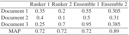
A toy example shown in Table 1 describes this problem. According to the ranking scores, the ranking lists returned by Ranker 1 and 2 are {2,1,3} and{3,1,2}, respec-tively, and the corresponding MAPs are 0.72 and 0.72. In order to make full use of the ranking information provided by both rankers, a conventional heuristic is to sum up rank-ing scores (i.e., use uniform weights,(0.5,0.5)), which generates Ensemble 1 with MAP equal to 0.72. Obviously, this procedure is not optimal since we can give arbitrary alter-native weights that generate a better precision. For example, Ensemble 2 uses weights
Table 1. A toy example. The values in the mid-three rows represent the ranking scores
given an identical query. The rankers are measured by MAP, as listed in the fifth row. The ranking scores of Ensemble 1 and 2 are defined by 0.5*Ranker 1+0.5*Ranker 2 and 0.7*Ranker 1+0.3*Ranker 2, respectively. The relevant document list is assumed to be
{2,3}.
Ranker 1 Ranker 2 Ensemble 1 Ensemble 2
Document 1 0.35 0.2 0.55 0.305
Document 2 0.4 0.1 0.5 0.31
Document 3 0.25 0.7 0.95 0.385
MAP 0.72 0.72 0.72 0.89
This toy example implies that there exist optimal weights assigned for the constituent rankers to construct an ensemble ranker. Different from proposing new probabilistic or nonprobabilistic models, this ensemble model motivates an alternative way for solving ranking tasks. In order to formulate this task as an optimization problem, the metric— MAP—is used as the objective function since it reflects the performance of IR system and tends to discriminate stably among systems compared to other IR metrics [18]. Therefore, our goal is changed to calculate the weights with which the MAP is maximized. In the following, we will describe and solve this problem mathematically.
2.2. Problem Definition
LetDbe a set of documents,Qa set of queries andΦa set of rankers.|Di|denotes the relevant document list,dj ∈Dthedthj document associated withjthrelevant document inDi,qi ∈ Qthe ith query andφk ∈ Φ thekth ranker. Lrepresents the number of queries,|Di|the number of relevant documents associated withqiandKφthe number of rankers. The ensemble ranker is defined asH = PKφ
k=1αkφk which linearly combines
Kφconstituent rankers with weightsα’s. We assume the relevant documents have been sorted in descending order according to the ranking sores. On the basis of these notations and the definition of MAP, the aforementioned problem can be formulated as:
max 1
L
L X
i
1
|Di|
|Di|
X
j
j R(dj, H)
s.t. Kφ
X
k=1
αk= 1
0≤αk≤1, k= 1,2, ..., Kφ
(P1)
whereR(dj, H)represents the ranking position of documentdj given by the ensemble modelH. In this constrained nonlinear program, a) the objective function is a general def-inition of MAP; and b) the constraints indicate that the linear combination is convex and that the weights can be interpreted as a distribution. Since the position functionR(dj, H) is defined by the ranking scores, it can be written as
R(dj, H) = 1 + X
d∈D,d6=dj
wheresx,y(H) = sx(H)−sy(H)andI{sx,y(H) <0}is an indicator function which equals 1 ifsx,y(H)<0is true and 0 otherwise. Here,sx(H)denotes the ranking score of documentxgiven by ensemble modelH andsx,y(H)the difference of the ranking scores between documentxandy. Sincesx(H)is linear with respect to the weights, it can be rewritten as
sx(H) =sx
Kφ
X
k=1
αkφk(qi)
=
Kφ
X
k=1
αksx(φk(qi))
(2)
wheresx(φk(qi))denotes the relevant score of documentxfor queryqi calculated by modelφk.
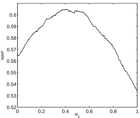
Here, we give an example illustrating the graph of the objective function. This exam-ple employed the MED data set with the settings identical to those in [16] except that only two constituent rankers, LDI and pLSI, were used to comprise the ensemble ranker for plotting purpose. The weights were restricted to the constraints in Problem P1 with the precision of three digits after the decimal point. In detail, the objective function was evaluated by settingα1for LDI andα2for pLSI, whereα1+α2= 1, andα1increased from 0to1 with a step size of0.001. Figure 1 shows a partial of the graph of objec-tive function. From this plot, it is clearly observed that a) the objecobjec-tive function is highly nonsmooth and nonconvex; and b) there are numerous local optimums in the objective function. Though the differentiability is not obvious in this graph, the position function implies that the objective function is nondifferentiable in terms of weights. Therefore, the general gradient-based algorithms, such as Lagrangian Relaxation and Newton’s Method, cannot be applied to this problem directly to find the optimum, even local optimums [3].
From this analysis of the objective function, the position function plays an important role in the differentiability. Thus, we will discuss how to approximate it with a differen-tiable function and how to solve this optimization Problem P1 in the next two sections.
3.
Approximation
In this section, we propose a differentiable surrogate for the position function and further approximate the Problem P1 with an easier nonlinear program.
Since the position function is defined by an indicator function (Equation 1), we can use a sigmoid function to approximate this indicator function, i.e.,
I{sdj,d(H)<0} ≃
exp(−βsdj,d(H))
1 + exp(−βsdj,d(H))
, (3)
whereβ >0is a scaling constant. It is obvious that this approximation is in the range of
[0.5,1)ifsdj,d(H)≤0and(0,0.5]ifsdj,d(H)>0. The following theorem shows that
we can get a tight bound by this approximation.
Theorem 1. The difference between the sigmoid functiongij and the indicator function
I{sdj,d(H)<0}is bounded as:
gij−I{sdj,d<0} <
0 0.2 0.4 0.6 0.8 1 0.52
0.53 0.54 0.55 0.56 0.57 0.58 0.59 0.6
α1
MAP
Fig. 1. An illustrated example of the objective function with two constituent rankers in
Problem P1.
whereδij = min|sdj,d|,gij =
exp(−βPKφk=1αksdj ,d)
1+exp(−βPKφk=1αksdj ,d)
andsdj,drepresentssdj,d(φk(qi))
for notational simplicity henceforth
Proof. Forsdj,d>0, we haveI{sdj,d<0}= 0andδij≤sdj,d, thus,
gij−I{sdj,d<0}
≤
1 1 + exp(βδijP
Kφ
k=1αk) Forsdj,d<0, we haveI{sdj,d<0}= 1andδij≤ −sdj,d, thus,
gij−I{sdj,d<0}
≤ 1
1 + exp(βδijP Kφ
k=1αk)
SincePKφ
k=1αk = 1, we can get
gij−I{sdj,d<0}
≤
1 1 + exp(βδij)
. (4)
This completes the proof.
This theorem tells us that the sigmoid function is asymptotic to the indicator function especially whenβis chosen to be large enough. By using this approximation, the position function can be correspondingly approximated as
ˆ
R(dj, H) = 1 + X
d∈D,d6=dj
exp(−βsdj,d(H))
1 + exp(−βsdj,d(H))
which becomes differentiable and continuous.
Then it is trivial to show the approximation error of position function, i.e.,
Rˆ(dj, H)−R(dj, H) ≤
X
d∈D,d6=dj
gij−I{sdj,d<0}
< |D| −1
1 + exp(βδij)
.
(6)
Suppose 1000 documents exit in the document set D and δij = 0.04. By setting
β= 300, the approximation error of the position function is bounded by
Rˆ(dj, H)−R(dj, H)
<0.006, (7)
which is tight enough for our problem.
In this way, the original Problem P1 can be approximated by the following problem
max 1
L
L X
i=1
1
|Di|
|Di|
X
j=1
j
ˆ
R(dj, H)
s.t. Kφ
X
k=1
αk = 1
0≤αi≤1, i= 1,2, ..., Kφ.
(P2)
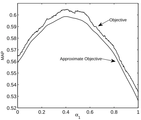
Using the settings identical to Figure 1, Figure 2 plots the graphs of the original ob-jective function (OOF) in Problem P1 and the approximated obob-jective function (AOF) in Problem P2. As shown in the plot, the trend of the AOF is close to that of the OOF. The weights generating the optimal MAP almost remain unchanged in these two curves. From this example, it is illustratively shown that the original noncontinuous and non-differentiable objective function can be effectively approximated by a continuous and differentiable function. The following lemma and theorem will theoretically prove this conclusion.
Theorem 2. The error between the OOF in Problem P1 and the AOF in Problem P2 is
bounded as
|Λˆ−Λ|< (|D| −1)(L+
P i|Di|)
2L(1 + exp(βδij))
(8)
whereΛˆandΛdenote the objective function in Problem P2 and Problem P1, respectively.
Proof. For the approximation error, we have
|Λˆ−Λ|= 1
L
L X
i=1
1
|Di|
|Di|
X
j=1
j(R−Rˆ)
RRˆ
0 0.2 0.4 0.6 0.8 1 0.52
0.53 0.54 0.55 0.56 0.57 0.58 0.59 0.6
α1
MAP Approximate Objective
Objective
Fig. 2. Comparison of the OOF in Problem P1 and AOF in Problem P2. (β= 200)
whereRdenotesR(dj, H)for notational simplicity. SinceRˆ = 1 +Pd6=djgij(α)and
R= 1 +P
d6=djI{sdj,d<0}are strictly positive, we have
j(R−Rˆ)
RRˆ
=
j R−Rˆ
RRˆ .
According to Equation 6, we have
|Λˆ−Λ|< (|D| −1)(L+
P i|Di|)
2L(1 + exp(βδij))
. (9)
This completes the proof.
This theorem indicates that the OOF in Problem P1 can be accurately approximated by the surrogate defined by the position function (5) in Problem P2. For example, if|D| = 10000,L = 200,P
|Di| = 500,β = 300andδij = 0.04, the absolute discrepancy between the objectives in Problem P1 and P2 is bounded by
|Λˆ−Λ|<0.1.
This discrepancy is within an acceptable level and will decrease with the growth of the query sizeLand the value ofβ.
rankers. However, adding constraints increases the difficulty of solving this optimization problem. Intuitively, the normalization of weights assigned for ranking scores is nonessen-tial because the ranking position is determined by the relative values of ranking scores. Take the toy in Table 1 as an example, the weights(3.5,1.5)result in the identical En-semble 2 to(0.7,0.3). The lemmas and theorems below prove the hypothesis that this constrained nonlinear program can be approximated by an unconstrained nonlinear pro-gram.
Lemma 1. Problem P2 is equivalent to the following problem:
max 1
L
L X
i=1
1
|Di|
|Di|
X
j=1
j
˜
R (P3)
whereR˜= 1+P
d∈D,d6=dj˜gij,˜gij =
exp(−βPKφk=1α˜ksdj ,d(φk(qi)))
1+exp(−βPKφk=1α˜ksdj ,d(φk(qi)))
andα˜k = α ′
k PKφ
k=1α′k
, α′
k>
0, k= 1,2, ..., Kφ
SincePKφ
k=1α˜k= 1, it can be straightforwardly proved that Problem P3 is equivalent to Problem P2.
Remark 1. If we letg′
ij =
exp(−βPKφk=1α ′
ksdj ,d(φk(qi)))
1+exp(−βPKφk=1α′ksdj ,d(φk(qi)))
, Theorem 1 applies for bothg˜ij
andg′
ijas well.
The following theorem states that Problem P3 can be surrogated by an easier problem.
Theorem 3. Consider the following problem
max 1
L
L X
i=1
1
|Di|
|Di|
X
j=1
j
R′, (P4)
whereR′ = 1 +P
d∈D,d6=djg ′
ij. LetΛ˜andΛ′denote the objective function in Problem P3 and Problem P4, respectively. Then, we have the following bound for the absolute difference betweenΛ˜andΛ′
|Λ˜−Λ′|< ˆǫ(L+
PL i=1|Di|)
2L (10)
whereˆǫ=ǫ′+ ˜ǫ,ǫ′=|R′−R|and˜ǫ= R˜−R
.
Proof. From Lemma 1 and Lemma 1, we can derive the following bound.
|Λ˜−Λ′|
= 1
L
L X
i=1
1
|Di|
|Di|
X
j=1
j(R′−R˜) R′R˜
SinceR′= 1 +P d6=djg
′
ijandR˜= 1 + P
d6=dj˜gijare strictly positive, we have
jP
d6=djg ′
ij− P
d6=djg˜ij
(1 +P d6=djg
′
ij)(1 + P
d6=dj˜gij)
=j
P d6=dj
(gij′ −I{sdj,d<0}) + (I{sdj,d<0} −g˜ij)
(1 +P d6=djg
′
ij)(1 + P
d6=dj˜gij)
According to the general triangle inequality, we can draw an upper bound for the term in numerator
X
d6=dj
(gij′ −I{sdj,d<0}) + (I{sdj,d<0} −˜gij)
≤ X
d6=dj
gij′ −I{sdj,d<0}
+
X
d6=dj
I{sdj,d<0} −g˜ij
<ˆǫ.
Then, it is trivial to get
|Λ˜−Λ′|< 1 L
L X
i=1
1
|Di|
|Di|
X
j=1
j·ˆǫ
< ˆǫ(L+
PL i=1|Di|)
2L .
(11)
This completes the proof.
Since the differencesǫ′ andǫ˜are small enough, Problem P4 can accurately
approxi-mate Problem P3. This theorem tells us that the AOF is also determined by the ranking positions, i.e., the relative values of ranking scores, thus the normalization constraints in Problem P2 can be removed. Taking Lemma 1 and Theorem 2 into account, we can trivially draw the following corollary.
Corollary 1. Problem P1 can be approximated by Problem P4.
In the next section, we focus on proposing algorithms that solves Problem P4.
4.
Algorithm
In many IR environments such as recommendation systems in E-commerce, however, the queries and ranking scores are generated in real time so as to construct data sequences at different times. Thus, we will secondly propose an online algorithm, gEnM.ON, for dealing with these data sequences. The online algorithm is more scalable to large data sets with limited storage than the batch algorithm. In the online algorithm, the queries as well as corresponding ranking scores are input in a data stream and processed in a serial fashion.
A common assumption for the aforementioned frameworks is that the relevant docu-ments are known. However, the knowledge of relevant docudocu-ments are unknown in many modern IR systems such as search engines. For this IR environment, we further propose an unsupervised ensemble model, UnsEnM, which makes use of a co-training framework.
4.1. Batch Algorithm: gEnM.BAT
Although many sophisticated methods can be applied for finding a local optimum, we first propose a revised Newton’s method. Major modification includes the approximation of gradients and Hessian matrix.
For notational simplicity, we utilize:
Gij:= X
d∈D,d6=dj
gij′ ; (12)
Gkij:= X
d∈D,d6=dj
∂g′
ij
∂α′
k
; (13)
Gl ij:=
X
d∈D,d6=dj
∂g′
ij
∂α′
l
; (14)
Gkl ij :=
X
d∈D,d6=dj
∂2gij′
∂α′
k∂α′l
. (15)
Under those notations, the first and second derivative of the objective function in Prob-lem P4 can be written as
∂Λ′ ∂α′
k
= 1
L
L X
i=1
1
|Di|
|Di|
X
j=1
−jGk ij
(1 +Gij)2
, (16)
and
∂2Λ′ ∂α′
k∂α′l
=1
L
L X
i=1
1
|Di|
|Di|
X
j=1
−jGkl
ij(1 +Gij)2+ 2jGkijGlij(1 +Gij)
(1 +Gij)2
,
respectively. According to the second derivative, the Hessian matrix is defined by
H(α) =
∂2Λ′ ∂α′
1∂α′1
∂2Λ′ ∂α′
1∂α′2 · · · ∂2Λ′ ∂α′
1∂α′Kφ
∂2Λ′ ∂α′
2∂α′1
∂2Λ′ ∂α′
2∂α′2 · · · ∂2Λ′ ∂α′
2∂α′Kφ
..
. ... ...
∂2Λ′ ∂α′
Kφ∂α′1 ∂2Λ′ ∂α′
Kφ∂α′2 · · · ∂2Λ′ ∂α′
Kφ∂α′Kφ
. (18)
As stated by Theorem 6 in Appendix B, the addends in the first derivative can be estimated by zeros under certain conditions. This approximation also applies for the sec-ond derivative as well as the Hessian matrix since both contain the first derivative item. The advantages of using this approximation are two-fold: a) the computation of Hessian is simplified since many addends are set to zeros under certain conditions; and b) the computations ofGkjij,Gij,Glij andGkij can be carried out offline before evaluating the derivative and Hessian, which makes the learning algorithm inexpensive.
Since the objective function in Problem P4 is nonconvex, multiple local optimums may exist in the variable space. Therefore, different starting points are chosen to preclude the algorithm from getting stuck in one local optimum. The largest local optimum and the corresponding weights are returned as the final solutions. To accelerate the algorithm, we can distribute different starting points onto different cores for parallel computing.
The batch algorithm is summarized as follows. We note that αp and sdj,d(φ(qi))
represent the vectors with elements αp and sdj,d(φk(qi)), respectively, and that p =
1,2, ..., P indexesPinitial values.
Algorithm 1 gEnM.BAT (Generalized Ensemble Model by Revised Newton’s Algorithm
in Batch Setting.)
Require: Query setQ, document setD, relevant document set|Di|with respect toqi∈Q, ranking scoressd(φk(qi))with respect toithe query,kth methodφkand documentd∈D, a number of initial pointsαpand a thresholdǫ= 0for stopping the algorithm.
1: for eachαpdo
2: Set iteration countert= 1; 3: EvaluateΛ′t
; 4: repeat
5: Sett=t+ 1;
6: Compute gradient∇αtp−1Λ
′and Hessian matrixH(αt−1
p )(Algorithm 2); 7: Updateαtp=αtp−1+H(αtp−1)−1∇
αtp−1Λ ′;
8: EvaluateΛ′t; 9: untilΛ′t
−Λ′t−1< ǫ 10: Storeαt
p 11: end for 12: return α’s.
Algorithm 2 Approximated Derivative and Hessian Computation Algorithm.
Require: Query setQ, document setD, relevant document set|Di|with respect toqi∈Q, ranking scoressd(φk(qi))with respect toithe query,kth methodφkand documentd ∈ D, current
αtp−1.
1: forqi∈Qdo 2: fordj∈ |Di|do
3: SetGij,Gklij,GkijandGlijto zeros; 4: ford∈Ddo
5: sdj,d(φk(qi))←sdj(φk(qi))−sd(φk(qi));
6: g′
ij(αtp−1)←
exp(−βαtp−1sdj ,d(φ(qi))) 1+exp(−βαtp−1sdj ,d(φ(qi)));
7: Gij←Gij+gij′ (αtp−1)
8: if−2
β <α t−1
p sdj,d(φ(qi))<β2 then
9: Gkl
ij ← Gklij + β2sdj,d(φk(qi))sdj,d(φl(qi))g ′
ij(αtp−1)(1 − g′ij(αtp−1))(1 − 2g′
ij(αtp−1));
10: Gk
ij←Gkij+βsdj,d(φk(qi));
11: Gl
ij←Glij+βsdj,d(φl(qi));
12: else
13: Gkl
ij←Gklij;
14: Gkij←G
k ij;
15: Gl
ij←Glij;
16: end if
17: end for
18: end for
19: end for
20: Compute gradient∇αtp−1Λ
′ (Equation 40)
and Hessian matrixH(αtp−1); (Equation 18)
21: return ∇αtp−1Λ
′andH(αtp−1).
negative weights play a negative role in the ensemble model. Thus, the ignorance of those rankers are reasonable in practice.
4.2. Online Algorithm: gEnM.ON
In the previous two subsections, we have presented the learning algorithms for generating gEnM by batch data sets. In contrast to the batch setting, the online setting provides the gEnM a long sequence of data. The weights are calculated sequentially based on the data stream that consists of a series of time stepst = 1,2, ..., T. For example, the gEnM is constructed based on the new queries and corresponding rankings given at different times in a search engine. The final goal is also to maximize the overall MAP on the data sets.
max 1
T
T X
t=1
1
Dt Dt
X
j=1
j
1 +P
d∈D,d6=djg ′
ij
(19)
however, the overall complexity is extremely high since the batch algorithm should be run once at each time step.
In the online setting, the subsequent queries are not available at present. An alternative optimization technique should be considered to prevent from focusing too much on the present training data. To distinguish with the notation in the batch setting, we letxbe the query and supposex1,x2, ...xt, ...are the given query at timetin the online setting. Here, we assume that these sequences are given with the grand truth distributionp(x). Thus, the objective function of MAP can be defined as the expectation of average precision, i.e.,
J(α) =
∞
X
t=1
f(x, α)p(x)
= Ep[f(x, α)],
(20)
where
f(x, α) = 1
Dxt
Dxt X
j=1
j
1 +P
d∈D,d6=djg ′
xtj(α
′).
The expectation cannot be maximized directly because the truth distributionp(x)is unknown. However, we can estimate the expectation by the empirical MAP that simply uses finite training observations. A plausible approach for solving this empirical MAP op-timization problem is that using the stochastic gradient descent (SGD) algorithm which is a drastic simplification for the expensive gradient descent algorithm. Though the SGD algorithm is a less accurate optimization algorithm compared to the batch algorithm, it is faster in terms of computational time and cheaper in terms of storing memory [20, 21]. Another advantage is that the SGD algorithm is more adaptive to the changing environ-ment in which examples are given sequentially [22].
For our problem, the SGD learning rule is formulated as
αt+1=αt+ηt∇f(xt+1, αt) (21)
whereηtis called learning rate, i.e., a positive value depending ont. This updating rule is validated to increase the objective value at each step in terms of expectation, which can be verified by the following theorem.
Theorem 4. Using the updating rule (21), the expectation of average precision increases
at each step, i.e.,
Ep[f(x, αt+1)]≥Ep[f(x, αt)]
Proof. SinceEp[f(x, αt+1)]−Ep[f(x, αt)] = Ep[f(x, αt+1)−f(x, αt)], we only need to showf(x, αt+1)−f(x, αt)≥0.
Since
f(x, αt+1)−f(x, αt) =
1
Dx Dx
X
j=1
jP
d6=dj(g ′
xj(α′t+1)−g′xj(α′t))
(1 +P d6=djg
′
xj(α′t+1))(1 + P
d6=djg ′
xj(α′t)) !
we need to verifyg′
xj(α′t+1)−gxj′ (α′t)≥0. According to the denotation ofg′ij, we have
gxj′ (α′t+1)−g′xj(α
′
t) =
τ(α′t)−τ(α′t+1)
(1 +τ(α′
t))(1 +τ(α′t+1))
whereτ(α′
t) = g′
xj(α′t)
1−g′
xj(α′t).
Since
τ(α′
t)
τ(α′
t+1)
= exp(βηt∇f(x, α′t)s(φ))
≥exp(0) = 1,
(22)
we can conclude that
τ(α′t)−τ(α′t+1)≥0.
This completes the proof.
The learning rateη plays an important role in the updating (Equation 22), hence an adequateηtwill enhance the online algorithm to converge. Defineηt= 1/tin this article, then we have the following well-known properties:
∞
X
t
ηt2<∞, (23)
∞
X
t
ηt=∞. (24)
Since it is difficult to analyze the whole process of online algorithm [20], we will show the convergence property around the global or local optimum in the following analysis.
Lemma 2. Ifαtis in the neighborhood of the optimumα∗, we have
(αt−α∗)∇f(x, αt)<0. (25)
The proof of is straightforward referring to Equation 35. This lemma states that the gra-dient drives the current point towards the maximumα∗. In the stochastic process, the
following inequality holds
(αt−α∗)Ep[∇f(x, αt)]<0. (26)
Lemma 3. Ifαtis in the neighborhood of the optimumα∗, we have
lim
t→∞∇f(x, αt)
2<∞. (27)
The proof is given in the Appendix. For the stochastic nature, the expectation of
∇f(x, αt)2also converges almost surely, i.e.,
lim
t→∞Ep[∇f(x, αt)
Theorem 5 ( [23]). In the neighborhood of the maximumα∗, the recursive variablesα
converge to the maximum, i.e.,
lim
t→∞αt=α
∗. (29)
Proof. Define a sequence of positive numbers whose values measure the distance from the optimum, i.e.,
ht+1−ht= (αt−α∗)2. (30)
The sequence can be written as an expectation under the stochastic nature, i.e.,
Ep[ht+1−ht] = 2ηt(αt−α∗)Ep[∇f(x, αt)] +ηt2Ep[∇f(x, α)2] (31)
Since the first term on the right hand side is negative according to (26), we can obtain the following bound:
Ep[ht+1−ht]≤ηt2Ep[∇f(x, αt)2]. (32)
Conditions (24) and (28) imply that the right hand side converges. According to the quasi-martingale convergence theorem [24], we can also verify thathtconverges almost surely. This result implies the convergence of the first term in (31).
SinceP∞
t ηtdoes not converge according to (23), we can get
lim
t→∞(αt−α
∗)E
p[∇f(x, αt)] = 0. (33)
This result leads to the convergence of the online algorithm, i.e.,
lim
t→∞αt=α
∗.
This completes the proof.
Based on the learning rule (21), the online algorithm for achieving the ensemble model is summarized below.
4.3. Unsupervised Algorithm: UnsEnM
Algorithm 3 gEnM.ON (Generalized Ensemble Model by Online Algorithm.)
Require: Query setQ, document setD, relevant document set|Di|with respect toqi∈Q, ranking scoressd(φk(qi))with respect toithe query,kth methodφkand documentd∈D, a number of initial pointsαpand a thresholdǫ >0for stopping the algorithm.
1: for eachαpdo
2: Set iteration countert= 1; 3: EvaluateΛ′t;
4: repeat
5: for eachqi∈Qdo 6: Sett=t+ 1;
7: Compute gradient∇αtp−1Λ
′with respect toq
i (Algorithm 2);
8: Updateαtp=αtp−1+1
t∇αtp−1Λ ′;
9: end for
10: EvaluateΛ′t; 11: until|Λ′t
−Λ′t−1|< ǫ 12: Storeαtp
13: end for 14: return α’s.
We modify the objective function in Problem P4 by adding a penalty item so that the refined ranking does not depend on the fake label too much. The modified objective function is defined as
max Λ′−1
2σ
X
qi∈Q
X
d∈D X
φk∈Φ
kHd(qi)−sd(φk(qi))k2 (P8)
whereHd(qi) =Pk
∈Kφ
k αksd(φk(qi)).
LetΓ denote the objective function in Problem P8. The second derivatives ofΓ can be written as follows:
∂Γ ∂αkαl
= ∂
2Λ′
∂αkαl
−σ X
qi∈Q
X
d∈D
(sd(φk(qi))·sd(φl(qi))) (34)
The approximation of Hessian matrix reported in Algorithm 2 can be employed here, however, it is time-consuming doing so since the unsupervised algorithm requires a large number of iterations to converge and the Hessian should be calculated at each iteration. Therefore, the learning rule of the online algorithm gEnM.ON is applied for the unsuper-vised algorithm. It is noteworthy that the gEnM.ON can be effortlessly modified to fit this unsupervised co-training scheme. The algorithm is described below.
5.
Empirical Experiment
5.1. Experiment Setup
Algorithm 4 UnsEnM (Unsupervised Ensemble Model.)
Require: Query setQ, document setD, ranking scoressd(φk(qi))with respect toithe query,kth methodφkand documentd∈D, a number of initial pointsαp, a thresholdǫsforsd(φk(qi))
to choose fake relevant documents and a thresholdǫ >0for stopping the algorithm. 1: for eachαpdo
2: Set iteration countert= 1; 3: EvaluateΛ′t;
4: repeat
5: for eachφk∈Φdo 6: Sett=t+ 1;
7: Refresh fake relevant document set|Di|=∅; 8: Constructsˆdthat excludessd(φk);
9: Constructαpthat excludesαφ
k;
10: forqi∈Qdo
11: ifsd(φk(qi))> ǫsthen
12: Construct fake relevant document set|Di| ←i∪ |Di|;
13: end if
14: end for
15: Compute gradient∇αtp−1Λ
′; (Algorithm 2)
16: Updateαtp=αtp−1+1
t∇αtp−1Λ ′;
17: end for
18: Reconstructαpthat includesαφ
k;
19: EvaluateΛ′t ; 20: until|Λ′t−Λ′t−1|< ǫ 21: Storeαtp
22: end for 23: return α’s.
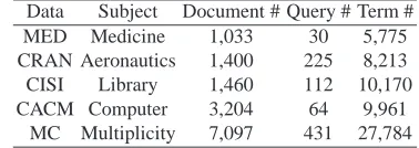
SMART IR System3. In order to test the proposed methods on heterogeneous data, we utilized the merged collection (MC) advocated by [16], which combines the four col-lections. The basic statistics of the test data are summarized in Table 2. The following minimum pre-processing measures were taken for the collections before evaluating the proposed methods: a) stop words were removed from the corpus by referring to a list of 571 stop words provided by SMART1; b) special symbols, including hyphenation marks, were removed; and c) those words with unique appearances in the corpus were removed. We note that the incomplete documents and queries in CISI and CACM were retained in the experiments.
The constituent rankers, in essence, are important factors that influence the results. Four rankers recommended by [16], namely tf-idf -based ranker (TFIDF) [1], Latent Se-mantic Analysis (LSA) [25], probabilistic Latent SeSe-mantic Indexing (pLSI) [26], Indexing by Latent Dirichlet Allocation (LDI) [16], were utilized in this paper for assembling the gEnM. In brief, TFIDF represents documents by a tf-idf weighted matrix; LSA projects each document into a lower dimensional conceptual space by applying Singular Value Decomposition (SVD); pLSI is a probabilistic version of LSA; and LDI represents each document by a probabilistic distribution over shared topics based on Latent Dirichlet
Al-3
Table 2. Data characteristics.
Data Subject Document # Query # Term #
MED Medicine 1,033 30 5,775
CRAN Aeronautics 1,400 225 8,213 CISI Library 1,460 112 10,170 CACM Computer 3,204 64 9,961
MC Multiplicity 7,097 431 27,784
location (LDA) [27]. These rankers are all unsupervised rankers and thus are trivial to be trained in the unsupervised setting. In addition to this training requirement, the rankers contain different information describing each corpus, such as information of keyword matching, concepts, or topics.
Since the four rankers represent documents and queries into vectors, the ranking scores are the cosine distances (or cosine similarities) between the vectors of documents and queries. Subsequently, the ranking scores of gEnM can be generated with appropri-ate adjustments to the weights being made for the ranking scores of the four rankers. For formulating Problem P4, we setβ = 200. Finally, the proposed algorithms can be implemented to calculate the optimal weights for gEnM.
In order to address the over-fitting problem of batch algorithms, we adopted the two-fold cross validation for testing the gEnM.BAT and gEnM.ON. A difference for the gEnM.ON is that the training queries and corresponding relevant documents were given sequentially at each step. The performance metric was the mean value of the MAPs in the two-fold cross validation. As for the UnsEnM, the ranking scores of different constituent rankers are provided as labeled data for other rankers in different rounds. The UnsEnM was then evaluated by means of MAP on the real labeled data.
As discussed in Section 4, the proposed algorithms would benefit from different initial weights. Choosing the proper initial points for nonlinear program is an open research is-sue. In our tests, we utilized the operational criterion of selecting the best. In other words, we tested performances for different initial weights and selected the one that generated the maximum retrieval performance in terms of MAP. In this experiment, we first set the initial weights to binary elements, i.e.,α ∈ B4. The reason of doing so lies in that the constituent rankers are initially active in some of the rankers and inactive in others, which reflects our heuristics at the first step. Since the EnM has been shown prior to the four basis rankers by [16], the EnM model was used as baseline methods for comparison.
5.2. Experimental Results
In other words, the retrieved documents by gEnM are more relevant at high ranking posi-tions, which is desirable from the user’s point of view.
Table 3. Comparison of the algorithms for gEnM and baseline methods. Pr@1 denotes
the precision at one document and Pr@5 the precision at five documents. An asterisk (*) indicates a statistically significant difference between EnM and gEnM.BAT with a 95% confidence according to the Wilcoxon signed rank test.
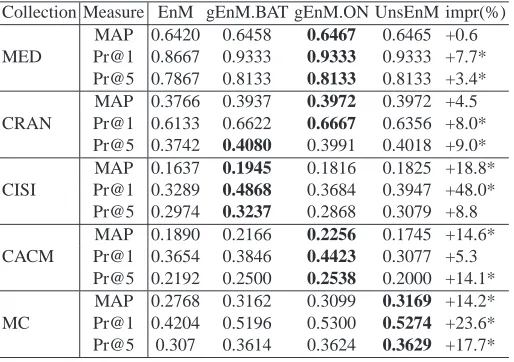
Collection Measure EnM gEnM.BAT gEnM.ON UnsEnM impr(%) MED
MAP 0.6420 0.6458 0.6467 0.6465 +0.6 Pr@1 0.8667 0.9333 0.9333 0.9333 +7.7* Pr@5 0.7867 0.8133 0.8133 0.8133 +3.4* CRAN
MAP 0.3766 0.3937 0.3972 0.3972 +4.5 Pr@1 0.6133 0.6622 0.6667 0.6356 +8.0* Pr@5 0.3742 0.4080 0.3991 0.4018 +9.0* CISI
MAP 0.1637 0.1945 0.1816 0.1825 +18.8* Pr@1 0.3289 0.4868 0.3684 0.3947 +48.0* Pr@5 0.2974 0.3237 0.2868 0.3079 +8.8 CACM
MAP 0.1890 0.2166 0.2256 0.1745 +14.6* Pr@1 0.3654 0.3846 0.4423 0.3077 +5.3 Pr@5 0.2192 0.2500 0.2538 0.2000 +14.1* MC
MAP 0.2768 0.3162 0.3099 0.3169 +14.2*
Pr@1 0.4204 0.5196 0.5300 0.5274 +23.6*
Pr@5 0.307 0.3614 0.3624 0.3629 +17.7*
From Table 3, we also see that the performance of gEnM.ON is better than the gEnM.BAT. The slight priority of gEnM.ON is due to the approximation of Hessian for the gEnM.BAT. However, the gEnM.ON is more expensive than gEnM.BAT because of iterative use of queries for calculation. Having said that, gEnM.ON can be used in a specific system where data are given in sequence. Since the knowledge of relevant documents is unknown in un-supervised learning, the performance of UnsEnM is inferior to the un-supervised algorithms. However, the results on the more heterogeneous data set MC are surprisingly the best among the proposed algorithms. The supervised algorithm may work well when tested against similar queries and documents in the homogeneous data. Yet the unsupervised al-gorithm does not fit the training data as much as the supervised alal-gorithm does and thus the superiority becomes more obvious when tested on more heterogeneous data.
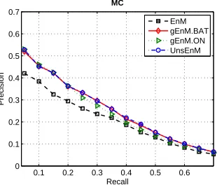
Figure 3 shows the precision-recall curves of the examined methods.
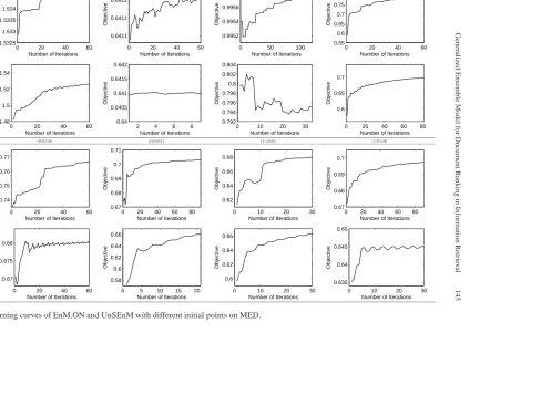
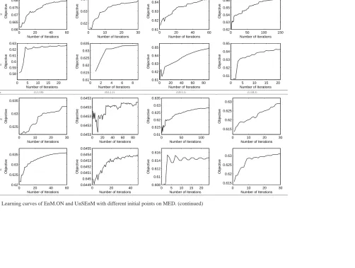
For illustrating the learning abilities of the gEnM.ON and UnsEnM, the learning curves on the MED data are reported in Figure 4. The results on the other data sets are very similar. The tolerance is set to1e−4and the number of iteration is set to at least
mit-0 0.1 0.2 0.3 0.4 0.5 0.6 0.5
0.6 0.7 0.8 0.9 1
Recall
Precision
MED
EnM gEnM.BAT gEnM.ON UnsEnM
0.1 0.2 0.3 0.4 0.5 0.6 0.7 0
0.1 0.2 0.3 0.4 0.5 0.6 0.7 0.8
Recall
Precision
CRAN
EnM gEnM.BAT gEnM.ON UnsEnM
0.1 0.2 0.3 0.4 0.5 0.6 0.7 0
0.1 0.2 0.3 0.4 0.5
Recall
Precision
CISI
EnM gEnM.BAT gEnM.ON UnsEnM
0 0.1 0.2 0.3 0.4 0.5 0.6 0
0.1 0.2 0.3 0.4 0.5
Recall
Precision
CACM
EnM gEnM.BAT gEnM.ON UnsEnM
Fig. 3. Precision-Recall Curves for the testing data sets.
0.1 0.2 0.3 0.4 0.5 0.6 0
0.1 0.2 0.3 0.4 0.5 0.6 0.7
Recall
Precision
MC
EnM gEnM.BAT gEnM.ON UnsEnM
Fig. 3. Precision-Recall Curves for the testing data sets. (continued)
igate due to the majority effect. Apart from these specific cases, the gEnM.ON is able to gradually learn from the sequences, which is consistent with the theoretical analysis.
out by other rankers. As a matter of fact, this phenomenon is similar to gEnM.ON since the data are given sequentially in both cases.
6.
Conclusions and Discussions
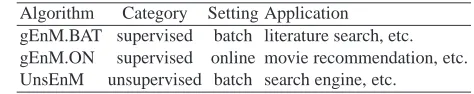
In this paper, we propose a generalized ensemble model, gEnM, which tries to find the op-timal linear combination of multiple constituent rankers by directly optimizing the prob-lem defined based on the mean average precision. In order to solve this optimization problem, the algorithms are devised in two aspects, i.e., supervised and unsupervised. In addition, two settings for the data are considered in the supervised learning, namely batch and online setting. Table 4 summarises the algorithms with potential applications in prac-tice. In brief, the gEnM.BAT can be used in those IR systems that have the knowledge of labeled data, such as academic search engines; the gEnM.ON is appropriate for real-time systems where the data is given in sequence, such as movie recommendation systems; and the UnsEnM is proposed for those systems without the knowledge of labeled data, such as search engines.
Table 4. Summary of the algorithms: gEnM.BAT, gEnM.ON and UnsEnM.
Algorithm Category Setting Application gEnM.BAT supervised batch literature search, etc. gEnM.ON supervised online movie recommendation, etc. UnsEnM unsupervised batch search engine, etc.
An experimental study was conducted based on the public data sets. The encourag-ing results verify the effectiveness of the proposed algorithms for both homogeneous and heterogeneous data. The gEnM performance is always better than the EnM, except for the case of UnsEnM on CACM. Briefly, the difference between gEnM.BAT and EnM is statistically significant in most cases; the gEnM.ON performs the best among the pro-posed algorithms for the MED, CRAN and CACM; and the unsupervised UnsEnM is more applicable for heterogeneous data than the supervised algorithms.
While we have shown the effectiveness of the proposed algorithms, we have not yet analyzed the computational complexity of the algorithms. Though we simplified the com-putation of the derivative and Hessian matrix, we were unable to reduced the complexity of the batch algorithm based on Newton’s method. A possible future direction is to ex-ploit cheaper and faster algorithms for the batch setting. Another interesting research topic is the selection of initial weights, which is actually an open research issue in nonlinear programming.
G en er al iz ed E n se m b le M o d el fo r D o cu m en t R an k in g in In fo rm at io n R et rie v al 1 4 5 gEnM.ON
0 20 40 60
1.5325 1.533 1.5335 1.534 1.5345
Number of Iterations
Objective
0 20 40 60
0.6411 0.6411 0.6412
Number of Iterations
Objective
0 50 100
0.9952 0.9954 0.9956 0.9958
Number of Iterations
Objective
0 20 40 60
0.55 0.6 0.65 0.7 0.75 0.8
Number of Iterations
Objective
UnsEnM
0 20 40 60
1.48 1.5 1.52 1.54
Number of Iterations
Objective
2 4 6 8
0.64 0.6405 0.641 0.6415 0.642
Number of Iterations
Objective
0 10 20 30
0.792 0.794 0.796 0.798 0.8 0.802 0.804
Number of Iterations
Objective
0 20 40 60 80
0.6 0.65 0.7
Number of Iterations
Objective
Initialα (0;0;1;0) (0;0;0;1) (1;1;0;0) (1;0;1;0)
gEnM.ON
0 20 40 60
0.74 0.75 0.76 0.77
Number of Iterations
Objective
0 20 40 60 80
0.67 0.68 0.69 0.7 0.71
Number of Iterations
Objective
0 10 20 30
0.62 0.64 0.66 0.68
Number of Iterations
Objective
0 20 40 60 80
0.67 0.68 0.69 0.7
Number of Iterations
Objective
UnsEnM
0 20 40 60
0.67 0.675 0.68
Number of Iterations
Objective
0 5 10 15 20
0.58 0.6 0.62 0.64 0.66
Number of Iterations
Objective
0 10 20 30
0.6 0.62 0.64 0.66
Number of Iterations
Objective
0 10 20 30
0.635 0.64 0.645 0.65
Number of Iterations
Objective
1 4 6 Y an sh an W an g et al . gEnM.ON
0 20 40 60
0.66 0.665 0.67 0.675 0.68 0.685
Number of Iterations
Objective
0 10 20 30
0.62 0.63 0.64
Number of Iterations
Objective
0 20 40 60
0.61 0.62 0.63 0.64 0.65
Number of Iterations
Objective
0 50 100 150
0.62 0.63 0.64 0.65 0.66 0.67
Number of Iterations
Objective
UnsEnM
0 5 10 15 20
0.58 0.59 0.6 0.61 0.62 0.63
Number of Iterations
Objective
0 2 4 6 8
0.61 0.615 0.62 0.625 0.63 0.635
Number of Iterations
Objective
0 20 40 60 80
0.61 0.62 0.63 0.64 0.65
Number of Iterations
Objective
0 5 10 15 20
0.61 0.62 0.63 0.64 0.65
Number of Iterations
Objective
Initialα (1;1;1;0) (0;1;1;1) (1;0;1;1) (1;1;0;1)
gEnM.ON
0 10 20 30
0.625 0.63 0.635
Number of Iterations
Objective
0 20 40 60 80
0.6453 0.6453 0.6453 0.6453 0.6453
Number of Iterations
Objective
0 50 100
0.61 0.615 0.62 0.625 0.63 0.635
Number of Iterations
Objective
0 10 20 30
0.615 0.62 0.625 0.63
Number of Iterations
Objective
UnsEnM
0 20 40 60
0.62 0.625 0.63 0.635
Number of Iterations
Objective
0 20 40
0.6449 0.645 0.6451 0.6452 0.6453 0.6454 0.6455
Number of Iterations
Objective
0 5 10 15 20
0.608 0.61 0.612 0.614 0.616
Number of Iterations
Objective
0 10 20 30
0.615 0.62 0.625 0.63
Number of Iterations
Objective
References
1. Salton, G., McGill, M.J.: Introduction to modern information retrieval. McGraw-Hill, Inc. (1986)
2. J¨arvelin, K., Kek¨al¨ainen, J.: Ir evaluation methods for retrieving highly relevant documents. In: Proceedings of the 23rd annual international ACM SIGIR conference on Research and development in information retrieval, ACM (2000) 41–48
3. Qin, T., Liu, T.Y., Li, H.: A general approximation framework for direct optimization of infor-mation retrieval measures. Inforinfor-mation retrieval 13(4) (2010) 375–397
4. Xu, J., Liu, T.Y., Lu, M., Li, H., Ma, W.Y.: Directly optimizing evaluation measures in learning to rank. In: Proceedings of the 31st annual international ACM SIGIR conference on Research and development in information retrieval, ACM (2008) 107–114
5. Yue, Y., Finley, T., Radlinski, F., Joachims, T.: A support vector method for optimizing average precision. In: Proceedings of the 30th annual international ACM SIGIR conference on Research and development in information retrieval, ACM (2007) 271–278
6. Chapelle, O., Le, Q., Smola, A.: Large margin optimization of ranking measures. In: NIPS Workshop: Machine Learning for Web Search. (2007)
7. Taylor, M., Guiver, J., Robertson, S., Minka, T.: Softrank: optimizing non-smooth rank metrics. In: Proceedings of the international conference on Web search and web data mining, ACM (2008) 77–86
8. Guiver, J., Snelson, E.: Learning to rank with softrank and gaussian processes. In: Proceed-ings of the 31st annual international ACM SIGIR conference on Research and development in information retrieval, ACM (2008) 259–266
9. Freund, Y., Schapire, R.E.: A desicion-theoretic generalization of on-line learning and an ap-plication to boosting. In: Computational learning theory, Springer (1995) 23–37
10. Hashemi, H.B., Yazdani, N., Shakery, A., Naeini, M.P.: Application of ensemble models in web ranking. In: Telecommunications (IST), 2010 5th International Symposium on, IEEE (2010) 726–731
11. Hoi, S.C., Jin, R.: Semi-supervised ensemble ranking. In: AAAI. (2008) 634–639
12. Wang, Y., Wu, S., Li, D., Mehrabi, S., Liu, H.: A part-of-speech term weighting scheme for biomedical information retrieval. Journal of Biomedical Informatics 63 (2016) 379–389 13. Xu, J., Li, H.: Adarank: a boosting algorithm for information retrieval. In: Proceedings of the
30th annual international ACM SIGIR conference on Research and development in information retrieval, ACM (2007) 391–398
14. Wu, Q., Burges, C.J., Svore, K.M., Gao, J.: Adapting boosting for information retrieval mea-sures. Information Retrieval 13(3) (2010) 254–270
15. Burges, C.J., Svore, K.M., Bennett, P.N., Pastusiak, A., Wu, Q.: Learning to rank using an ensemble of lambda-gradient models. In: Yahoo! Learning to Rank Challenge. (2011) 25–35 16. Wang, Y., Lee, J.S., Choi, I.C.: Indexing by latent dirichlet allocation and an ensemble model.
Journal of the Association for Information Science and Technology 67(7) (2016) 1736–1750 17. Wei, F., Li, W., Liu, S.: irank: A rank-learn-combine framework for unsupervised ensemble
ranking. Journal of the American Society for Information Science and Technology 61(6) (2010) 1232–1243
18. Robertson, S.: On smoothing average precision. In: Advances in Information Retrieval. Springer (2012) 158–169
19. Wang, J., Kwon, S., Shim, B.: Generalized orthogonal matching pursuit. IEEE Transactions on signal processing 60(12) (2012) 6202–6216
20. Murata, N.: A statistical study of on-line learning. Online Learning and Neural Networks. Cambridge University Press, Cambridge, UK (1998)
22. Amari, S.: A theory of adaptive pattern classifiers. Electronic Computers, IEEE Transactions on (3) (1967) 299–307
23. Bottou, L.: Online learning and stochastic approximations. Online Learning and Neural Net-works (1998)
24. Fisk, D.L.: Quasi-martingales. Transactions of the American Mathematical Society 120(3) (1965) 369–389
25. Deerwester, S.C., Dumais, S.T., Landauer, T.K., Furnas, G.W., Harshman, R.A.: Indexing by latent semantic analysis. Journal of the American Society for Information Science 41(6) (1990) 391–407
26. Hofmann, T.: Probabilistic latent semantic indexing. In: Proceedings of the 22nd Annual International ACM SIGIR Conference on Research and Development in Information Retrieval, ACM (1999) 50–57
27. Blei, D.M., Ng, A.Y., Jordan, M.I.: Latent dirichlet allocation. Journal of Machine Learning Research 3 (2003) 993–1022
A.
Derivation of the derivative of
Λ
′(1) Derivation of the first derivative
According to the calculus chain rule, the derivative of objective in Problem P4 with respect toαk, k = 1,2, .., Kφis
∂Λ′ ∂α′ k = 1 L L X i=1 1
|Di|
|Di|
X
j=1
−jP d6=dj
∂g′
ij
∂α′
k
(1 +P d6=djg
′
ij)2
, (35) where ∂g′ ij ∂α′ k
=−βsdj,d(φk(qi))g ′
ij(1−g
′
ij). (36)
(2) Derivation of the second derivative
Also by the chain rule, the second derivative with respect toα′
l, l= 1,2, .., Kφis
∂2Λ′ ∂α′ k∂α ′ l = 1 L L X i=1 1
|Di|
|Di|
X
j=1
−jP ∂2g′ij
∂α′
k∂α′l(1 +
P
gij′ )2+ 2j P∂gij′
∂α′
k
P∂g′ij
∂α′
l(1 +
P
g′ij)
(1 +P d6=djg
′
ij)4
,
(37)
where
∂2g′
ij
∂α′
k∂α′l
=−βsdj,d(φk(qi))(1−2g ′ ij) ∂g′ ij ∂αl , (38) and∂g ′ ij
∂αl can be calculated by Equation 36.
B.
Approximation of the derivative of sigmoid function
For notational simplicity, we begin by considering the following sigmoid function:
f(x) = 1
Theorem 6. The derivative of function (39) can be approximated as follows:
∂f(x)
∂x ≃
−β(f(x)−f2(x)), if −2 β < x <
2
β;
0, ifx <−2
β orx >
2
β.
(40)
if the scaling constantβis large.
Proof. We apply the centered linear approximation method to the approximation of the sigmoid function as shown in Figure 5, which is described below:
f(x)≃
f(x), if −2 β < x <
2
β;
0, ifx <−2 β;
1, ifx > 2 β.
(41)
Hencef(x)(1−f(x)) = 0ifx <−2βorx > 2β. This completes the proof.
We note that this approximation is more precise with a largerβ.
(0,0) (−
2
β,1)
(2
β,0)
x y
(0,1)
Fig. 5. The approximation of sigmoid function through the centered linear
approxima-tion method. (β= 300)
Remark 2. The derivative function (36) can be approximated by:
∂gij′
∂α′
k
≃
−βsdj,d(φk(qi))g ′
ij(1−gij′ ),
if − 2 β <
X
k
α′ksdj,d(φk(qi))<
2
β;
0, otherwise.
(42)
C.
Proof of Lemma 3
In this section, we only sketch the proof of Lemma 3.
Proof (Sketch of Proof). In this proof, we use simple symbols for clarity. For example,
g(αt)denotesg′ij(α′t).
∇f(x, αt+1)2− ∇f(x, αt)2
= 1
D
D X
i=1
jβPsg(α
t+1)(1−g(αt+1))
(1 +P
d6=djg(αt+1))
2 !2
−
1
D
D X
i=1
jβP
sg(αt)(1−g(αt))
(1 +P
d6=djg(αt))
2 !2
< 1 D
D X
i=1
jβXsg(αt+1)(1−g(αt+1)) !2
Forg(αt+1)−g(αt+1)2, we have
g(αt+1)−g(αt+1)2< 1
2 + exp(βP
(αt+η∇f)s)
< 1
2 + exp(βP
η∇f s).
Thus, we have
∇f(x, αt+1)2− ∇f(x, αt)2<
1
D
D X
i=1
jβXs 1
2 + exp(βPη∇f s) !2
It is easy to show that the 1+exp(η)1 is the summand of a convergent infinite sum. This
result implies that ∇f(x, αt)2 converges because it is bounded and its oscillations are damped.
Yanshan Wang is currently a research fellow at Mayo Clinic, the No. 1 hospital in the
United States according to U.S. News and World Report Best Hospitals 2016-2017. He has been working on multiple projects including a R01 NIH funded project. He has over 20 research outcomes since he joined Mayo Clinic in 2015. Prior to joining Mayo Clinic, he received B.Eng. from Harbin Institute of Technology in 2010, M. Eng. and Ph.D. from Korea University in 2012 and 2015, respectively.
Chan Choi is a Professor at Korea University. He received his B.S. degrees in
tenure track faculty position in Industrial Engineering Department at Wichita State Uni-versity, Kansas, for five and half years. Outside academia, he has research work experi-ence at Bell Communications Research (Bellcore), where he was employed as a member of Technical Research Staff in 1988.
Hongfang Liu is a Professor in biomedical informatics at Mayo Clinic. She currently
leads the Biomedical Informatics group at Mayo Clinic. She has published extensively with over 200 research articles. Her current research missions are to facilitate secondary use of Electronic Health Records (EHRs) for clinical and translational science research and health care delivery improvement through clinical NLP and to deliver open-source NLP for high-throughput phenotyping through community-wide collaborative projects. She has led the community-wide project, Open Health Natural Language Processing (OHNLP; http://www.ohnlp.org), which promotes the release of open source NLP tools for clinical and translational research.