THINKING POKER THROUGH GAME THEORY

(1)

CSUSB ScholarWorks

Electronic Theses, Projects, and Dissertations Office of Graduate Studies

6-2016

Damian Palafox

Follow this and additional works at: https://scholarworks.lib.csusb.edu/etd

Part of the Other Applied Mathematics Commons, and the Probability Commons

Recommended Citation Recommended Citation

Palafox, Damian, "THINKING POKER THROUGH GAME THEORY" (2016). Electronic Theses, Projects, and Dissertations. 314.

https://scholarworks.lib.csusb.edu/etd/314

(2)

A Thesis

Presented to the

Faculty of

California State University,

San Bernardino

In Partial Fulfillment

of the Requirements for the Degree

Master of Arts

in

Mathematics

by

Damian Palafox

(3)

A Thesis

Presented to the

Faculty of

California State University,

San Bernardino

by

Damian Palafox

June 2016

Approved by:

Joseph Chavez, Committee Chair Date

Corey Dunn, Committee Member

Roland Trapp, Committee Member

Charles Stanton, Chair, Corey Dunn

Department of Mathematics Graduate Coordinator,

(4)

Abstract

Poker is a complex game to analyze. In this project we will use the mathematics

of game theory to solve some simplified variations of the game. Probability is the building

block behind game theory. We must understand a few concepts from probability such as

distributions, expected value, variance, and enumeration methods to aid us in studying

game theory. We will solve and analyze games through game theory by using different

decision methods, decision trees, and the process of domination and simplification. Poker

models, with and without cards, will be provided to illustrate optimal strategies.

Ex-tensions to those models will be presented, and we will show that optimal strategies still

exist. Finally, we will close this paper with an original work to an extension that can be

(5)

Acknowledgements

Dedicated to:

Joseph, professor, adviser, mentor, friend. Thank you for believing in this project.

Joyce, mentor and friend. Thank you for believing in me.

(6)

List of Tables

3.1 Products and Profits . . . 19

3.2 Opportunity Loss Table . . . 20

3.3 Current vs. Expansion . . . 21

3.4 Conditional Profits . . . 22

3.5 Expected Profit with Perfect Information . . . 23

4.1 Standard Matrix . . . 28

4.2 Game 1 . . . 29

4.3 Game 2 . . . 31

4.4 Game 2, Row Reduced . . . 32

4.5 Game 2, Row/Column Reduced . . . 32

4.6 Game 3 . . . 33

4.7 Algebraic 2 by 2 Matrix . . . 33

6.1 The Clairvoyance Game . . . 53

6.2 AKQ Game . . . 56

6.3 AKQ Game, Row Reduced . . . 57

6.4 AKQ Game, Row/Column Reduced . . . 58

6.5 AKQ Game, Simplified . . . 58

6.6 AKQ Game, Matrix Solution . . . 59

6.7 AKQ Game, Expected Values . . . 60

6.8 AKQ Game, Expected Values, Simplified . . . 60

6.9 AKQJ Game . . . 63

6.10 AKQJ Game, Reduced . . . 64

6.11 AKQJ Game, Simplified . . . 64

6.12 AKQJ Game, Expected Values . . . 70

6.13 AKQJ Game, Expected Values, Simplified . . . 71

6.14 AKQJ Game, Expected Values, Re-Simplified . . . 71

(9)

List of Figures

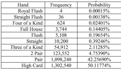
2.1 5-Card Poker Hands with Respective Probabilities. . . 12

3.1 Decision Tree Diagram. . . 23

3.2 Investment Opportunities. . . 25

5.1 La Relance. . . 38

5.2 von Neumann’s Poker Model. . . 42

5.3 von Neumann’s Poker Intervals. . . 42

5.4 Example 5.3.1 Intervals. . . 43

5.5 von Neumann’s Poker Extension 1. . . 46

5.6 von Neumann’s Poker Extension 1 Intervals. . . 46

5.7 Example 5.4.1 Solutions. . . 49

5.8 von Neumann’s Poker Extension 2. . . 50

(10)

Chapter 1

Introduction

There are many categories of poker games, and within each game category, there

are many variations, and even regional variants of the same game. Casinos could have

their own set of rules, while a home game could run the same game completely differently.

In general, poker games share some characteristics, there will be betting involved, and for

the most part a deck of 52 cards is used in play. In this sense, we can examine the game,

which may seem that involves randomness and luck, through a mathematical eye. This

will demonstrate that indeed, the game is solvable if we analyze it using game theory.

What are the tools needed for us to tackle this project?

In this expository paper we will present known solutions to simplified poker

models. Additionally, we will present original work extending some of these models.

Be-fore we can understand how the poker models work, some background work in probability

is required. Poker caters to some specific probability problems, those that fall into the

combinatorial spectrum. Our work in probability will lead us to understand one of the

most powerful concepts available to statisticians, Bayes’ Theorem. We will also need, as

the title of this project suggest, a grasp on game theory. Game theory has many

applica-tions in a wide array of fields such as economics, politics, psychology, science, computer

science, and biology to name a few. Although, we could spend an entire project studying

game theory alone, we will concentrate on decision making and solving 2-person games.

We can then think of Chapters 2 through 4 as an introductory stepping stone into the

world of poker. We will revise some old concepts while learning new ideas in the process.

(11)

Fer-guson & FerFer-guson, father and son, will provide an extensive look into the work of game

theorists ´Emile Borel and John von Neumann, about solving poker models. The poker

models provided will be reduced instances of an actual game with a well defined set of

rules. These poker models will also serve as a reminder that if a game is played optimally,

then a game can be profitable.

In the final chapter, we will attempt to apply game theory to a poker game.

Chen and Ankenman provide exhaustive work in their book, about how poker can be

solved step by step via mathematics. From their work we will take the game theoretical

approach to solving poker. We will start by extending the poker models of Chapter 5 to

an actual game of poker. Then, we will demonstrate how to reduce the whole game of

poker to a simple 3-card game that we can solve, and thus, we can play optimally. The

work done in Chapter 6 can then be applied to any other game, or specific circumstance

that we may encounter in real life.

In short, this project will not teach anyone how to play poker, but instead, we

(12)

Chapter 2

Probability

2.1

Probability

Game theory is the mathematical study of games. Game theory can be

di-vided into many branches, but it is usually defined as combinatorial or classical. The

combinatorial game theory is the branch that studies enumerations, combinations, and

permutations of sets of elements, and the mathematical relations that characterize their

properties. Understanding combinatorics is key in solving probability problems as they

arise in a game of poker. Probability is then defined as a real-valued set functionP that

assigns, to each event Ain the sample space S, a numberP(A), called the probability of

the event A, such that the following properties are satisfied:

(a) P(A)≥0.

(b) P(S) = 1.

(c) If A1, A2, A3, ... are events and Ai ∩Aj = ∅, i 6= j, then P(A1∪A2 ∪ · · · ∪Ak) =

P(A1) +P(A2) +· · ·+P(Ak) for each positive integerk, andP(A1∪A2∪A3∪ · · ·) =

P(A1) +P(A2) +P(A3) +· · · for an infinite, but countable, number of events [HT10].

Theorem 2.1. For each eventA, P(A) = 1−P(A0).

Proof. We have

S=A∪A0 and A∩A0 =∅.

Thus, from properties (b) and (c), it follows that

(13)

Hence,

P(A) = 1−P(A0).

[HT10].

We may also define probability as a number. If some number of n trials of an

experiment producesn0 successes, how many occurrences of an event xwill we have? As

nbecomes larger and grows without bound, this number will converge to a specific ratio,

thus the probability p of xoccurring p(x) times is the ratio

p(x) = lim n→∞

n0

n.

For example, what is the probability that we can draw a specific card from a

standard deck of cards? We first define a standard deck of cards as follows:

1. There are 52 cards.

2. There are 4 suits,♠ spades,♣clubs, ♥hearts, and ♦diamonds.

3. There are 13 ranks in each suit, A, 2, 3, 4, 5, 6, 7, 8, 9, 10, J, Q, K (The A, “Ace”

is both a high and low card in poker games).

4. Each card is unique, ie. there is only one 6 of clubs (6♣), and only one 8 of diamonds (8♦), etc.

It should be evident that the probability of drawing a specific card is then

1/52≈1.92% since each card is unique. If we wanted to draw any one card of any suit, say any club, we know that there are 13 clubs out of 52 possible cards, so 13/52 = 1/4 = 25%.

It should be clear that since the deck is divided into 4 equal suits, the probability of

drawing one card, of any one particular suit, is 25%. Another question we could ask is,

what is the probability of drawing any ace or any heart? We know that there are 4 aces

in the deck, and that there are 13 hearts in the deck, however, we must be careful and

not double count the A♥, this is the only card that can both be an ace and a heart at the same time. We can add the probabilities of a card being an ace, or a card being a heart,

(14)

there are 13 hearts and 4 aces and only one ace of hearts, so the probability of drawing

any ace or any heart is (₅₂13) + (₅₂4)−(₅₂1) = 16₅₂ ≈30.77%.

As demonstrated above, there could be many factors affecting probability and its

calculations. For some events, the occurrence of one event may not change the probability

of the occurrence of the other. Events of this type are said to be independent events.

The probability that both A and B occur is called the joint probability of A and B.

However, when one event has a clear impact on the other, that is, if event A happening

affects the probability of eventBoccurring, then it is said that the events aredependent.

We may also need to consider the conditional probability of A given B. This is the

probability that if event B happens, event A will also occur. In summary, we have the

following:

• EventsAandBareindependentif and only ifP(A∩B) =P(A)P(B). Otherwise,

A and B are calleddependent events.

• The conditional probability of an event A, given that event B has occurred is defined byP(A|B) =P(A∩B)/P(B) provided thatP(B)>0.

Throughout, we will use the following notation:

P(A∪B) = Probability of AorB occurring.

P(A∩B) = Probability of Aand B occurring.

P(A|B) = Conditional probability ofA occurring givenB has already occurred. For mutually exclusive events we have P(A∪B) =P(A) +P(B).

For all events P(A∪B) =P(A) +P(B)−P(A∩B). For independent events we have P(A∩B) =P(A)P(B). And for all events P(A∩B) =P(A)P(B|A).

Example 2.1.1 What is the probability that in rolling two fair dice, we can obtain a sum of 12?

We should note that we have two independent events, as the roll of one die will

not have any influence on the other. There is also only one way of obtaining a sum

of 12 from two dice, when both dice land on 6, which carries a 1/6 probability on

each die. Let P(A) be the probability that the first die is a 6, and letP(B) be the

probability that the second die is a 6. Then

(15)

Example 2.1.2 Three football players will attempt a field goal. LetAidenote the event that the field goal is made by player i, where, i = 1,2,3 and let P(A1) = 0.5,

P(A2) = 0.7,and P(A3) = 0.6. What is the probability that exactly one player is

successful? [HT10].

In this case we have three independent events, since one player, succeeding has no

affect on the others’ success or failure rate. We want to compute the probability of

one success and two failures, but we do not know which player will score and which

two will not. Therefore we must calculate the probability that if player 1 scores,

both player 2 and player 3 will miss. Also, since any player can score, we will do the

same for the other two cases, when player 2 scores the other two miss, and when

player 3 scores, both player 1 and player 2 miss. Now, we have

P(A1) +P(A10)→0.5 + 0.5 = 1,

P(A2) +P(A20)→0.7 + 0.3 = 1,

P(A3) +P(A30)→0.6 + 0.4 = 1.

We proceed to calculate,

P(A1∩A02∩A

0

3) +P(A

0

1∩A2∩A03) +P(A

0

1∩A

0

2∩A3)

=P(A1)P(A02)P(A03) +P(A01)P(A2)P(A03) +P(A10)P(A02)P(A3)

= (0.5)(0.3)(0.4) + (0.5)(0.7)(0.4) + (0.5)(0.3)(0.6)

= 0.06 + 0.14 + 0.09

= 0.29.

Example 2.1.3 Given a standard deck of cards, draw two cards without replacement, what is the probability that both cards will be aces?

We now have a pair of events that are dependent, since removing a card from the

deck will affect the probability of drawing the second card. Denote event A as the

first card is an ace, and eventBas the second card is also an ace. We know that the

probability of drawing one ace is 4/52 because there are 4 aces in a 52 card deck.

However, the probability of drawing a second ace is now 3/51, we have removed one

card from the deck, namely, an ace. Thus, for these dependent events

(16)

We will draw a pair of aces 1/221 ≈ 0.45% of the time. Now drawing two aces, or any other pair carries the same percentage. If this is the case, then what is the

probability that we can draw any pair? Since there are 13 ranks, we can have 13 types

of pairs. Then

13(₂₂₁1 ) = ₁₇1 ≈5.88%.

With these tools at our disposal, we can calculate any combination of cards

imaginable.

Example 2.1.4 Given a standard deck of cards, draw three cards without replacement, what is the probability that all cards will be of the same rank, that is three of a

kind?

As in the previous example, we have a set of dependent events. Let A denote the

event that the first card drawn is any card of any rank. Now B is the event where

second card is of the same rank asA, andC the event where the third card is of the

same rank as the previous two cards from Aand B. The probability of the events

are 52/52, 3/51, and 2/50 respectively. Then, for dependent events

P(A ∩ B ∩ C)

=P(A)P(B|A)P(C|B∩A)

= (52₅₂)(₅₁3)(₅₀2) = ₄₂₅1 ≈0.2%.

2.2

Distributions and Expected Value

More often than not, it is necessary to take into account many different

proba-bilities simultaneously. Possible outcomes and their respective probaproba-bilities can be

char-acterized by probability distributions. Probability distributions are created by taking

each outcome and pairing it with its probability.

• The probability distributionDof eventAwith probabilityP(A), and eventB with probability P(B), ... , and event Z with probability P(Z) is

D={(A, P(A)),(B, P(B)), ...,(Z, P(Z))},

(17)

For example, rolling a standard die yields the outcomes 1, 2, 3, 4, 5, or 6.

Each result happens 1/6 of the time. Thus the probability distribution of the roll is

D = {(1,1₆),(2,1₆),(3,1₆),(4,1₆),(5,₆1),(6,1₆)}. When a probability distribution is repre-sented by numerical values per every single outcome, we can find the expected value,

< EV >, of that distribution. EV is defined as the value of each outcome multiplied by

its probability, all summed together. In order to do well at any game, we must play in a

way that maximizes expected value.

Example 2.2.1 Roll a fair 6-sided die. We place a bet of one-unit on any particular number. A winning bet pays five-units when the dies lands on our chosen number,

otherwise, it is considered a losing bet, and we lose our bet of one-unit. What is

the expected value of this game? Is this a profitable game that we should play?

It does not matter which number we pick. We could pick always the number “2”

or we could change our number after every roll. Every single number has the same

probability of appearing. It is erroneous to think that a “4” is coming just because

it has not been observed in many rolls, or that “1” is the lucky number because that

number seems to repeat often. Therefore, let’s assume that we pick any number x

that has a 1/6 probability of showing. When we roll an x we will be paid 5 units,

however, we will lose 1 unit when any other of the five numbers show, which will

happen 5/6 of the time. The probability distribution is D={(5,1₆),(−1,5₆)}. The expected value of the game is < EV >= (1₆)(5) + (5₆)(−1) = 0.

Since the expected value of the game is 0, this is not a profitable game to play. If

we played this game long enough, we will never show a profit. Suppose we start by losing

some games, but winning just once will get us back to where we started. Or perhaps, we

could start by winning a few games, but eventually we will lose all of our profits and will

be back at zero. Note that if the payouts were changed to six-units per win, we will show

a profit of exactly 1/6 units or ≈0.16 units per unit played. If that were the case, we should be happy to play this game.

Example 2.2.2 Given a standard deck of cards, randomly draw a card. We place a bet of one-unit on any face card (any K, Q, J). If a face card is drawn we will win three-units, otherwise, we lose our initial bet. What is the probability distribution

(18)

The probability distribution is D ={(3,12₅₂),(−1,40₅₂)}. The expected value of the game is < EV >= (12₅₂)(3) + (40₅₂)(−1) = −0.07. This is a game that we should avoid since the expected value is negative.

The example above shows a characteristic of all casino games which are designed

to have negative expected values for the consumers. It should be noted that there are 12

face cards, any of which will win for us, and 40 non-face cards, which we lose to. There

is more than triple of the bad cards (3.33) than the good cards. We are only given 3 to 1

to our money, but we will lose more than that per game. We could in fact create our own

games, just like above, to give the consumer the illusion of being able to win big, when

in fact, they will lose overall. We may now formally define expected value of a random

variable X with probability distributionP as

< X >= n

X

i=1

pixi.

2.3

Enumeration

When working with probabilities, there may be a multitude of outcomes. So far

we have limited our experiments to six-sided dice, or a standard deck of 52 cards. Before

we can take on more complex or varied problems, we need to define some enumeration

techniques. The first and easiest is the multiplication principle. Suppose that a

procedure can be broken intomsuccessive (ordered) stages, withr1 different outcomes in

the first stage, r2 different outcomes in the second stage, ... , and rm different outcomes in the mth stage. If the number of outcomes at each stage is independent of the choices

in previous stages and if the composite outcomes are all distinct, then the total procedure

has (r1)(r2)· · ·(rm) different composite outcomes [Tuc02].

Example 2.3.1 In California, standard license plates for passenger vehicles are made up of one digit, followed by three letters, and ending with a three digit number.

Assuming that leading zeros are permissible, and that repetition is allowed, how

many different combinations of standard license plates are there?

Since there are 10 digits, 0-9, and 26 letters, a-z, available, the multiplication

prin-ciple gives

(19)

Example 2.3.2 In California, standard license plates for passenger vehicles are made up of one digit, followed by three letters, and ending with a three digit number.

Suppose leading zeros are not permissible, and repetition is not allowed on either

letters or numbers, now, how many different combinations of license plates are there

giving these restrictions?

There are 10 digits, 0-9, and 26 letters, a-z, available, the multiplication principle

gives

(9)(26)(25)(24)(9)(8)(7) = 70,761,600.

By having those restrictions, the total possible number of combinations was

reduced by 105 million possibilities. Let’s take a moment to discuss how the restrictions

affected the total number. The first factor is one of nine digits, 1-9, since 0 is not an

option. The second factor can be any of the 26 letters, whereas the third factor can

be any of the remaining 25 letters, because there is no repetition allowed. Similarly, the

fourth factor can consist of any of the remaining 24 letters. Now for the remaining factors,

the fifth factor can be any of the remaining nine digits, including zero but excluding the

leading digit of the license plate. Thus, the sixth and seventh factors have eight and seven

possible choices.

Another counting method is apermutation. Suppose that there arenpositions

which can be filled with n different objects. We can choose the first object in any of n

different ways,n−1 ways of choosing the second object,n−2 for the third, ... , and only one remaining way for the last object to be chosen. Thus by the multiplication principle

there are n(n−1)(n−2)· · ·(2)(1) = n! possible arrangements. Here n! is read as “n

factorial” where 0! = 1 [HT10].

Example 2.3.3 A soccer coach can field 11 players. Assuming that every player can play in any position, how many different line-ups are there available to the coach?

The coach can position the first player in any of the open 11 positions. The second

player in any of the remaining 10 positions, ... , the last player will fill the last open

position. Then there are

11! = (11)(10)· · ·(2)(1) = 39,916,800

(20)

Now, what if we had nobjects available and only need to fillr positions where

r < n? Then the number of possible arrangements is

nPr=n(n−1)(n−2)· · ·(n−r+ 1).

Here there are nways to fill the first position,n−1 ways to fill the second position, until only [n−(r−1)] = (n−r+ 1) ways of filling the rth position. Or

nPr=

n(n−1)· · ·(n−r+ 1)(n−r)· · ·(3)(2)(1) (n−r)· · ·(3)(2)(1) =

n! (n−r)!.

where each of the nPr arrangements is called a permutation of n objects taken r at

a time [HT10].

Example 2.3.4 How many ordered samples of five cards can be drawn without replace-ment from a standard deck of cards?

(52)(51)(50)(49)(48) = 52! (52−5)! =

52!

47! = 311,875,200.

In poker however, the order of selection is not important. If we have a pair of

aces, it does not matter in which manner we receive each card. We could get an ace as

the first card, and the last, fifth card could be the second ace. That hand will be equal

in value as if we had received both aces as our first two cards.

When we can disregard the order of selection of objects, since subsets are of

equal worth, we say that each of the nCr unordered subsets is called acombination of

n objects taken r at a time, where

nCr =

n r

= n!

r!(n−r)!.

Here nCr is read as “nchoose r” [HT10].

Example 2.3.5 What is the number of five-card hands of poker that can be made from a standard deck if we disregard order?

52C5 =

52 5

= 52!

5!47! = 2,598,960.

We can also calculate 52C5 as 52₅

(21)

Example 2.3.6 A poker hand is defined as drawing 5 cards at random without replace-ment from a standard deck of cards. What is the probability that the hand will

consist of one pair, that is two cards of the same rank and three different cards of

different ranks?

We first must choose one rank to make a pair. Since there are four cards of the

same rank, we can choose any two cards from that set. We then must be careful

and choose three cards, one from each of the remaining 12 ranks, where each can be

chosen from any of the four available cards. Otherwise we run the risk of making

either a second pair, or perhaps a three of a kind.

13 1 4 2 12 3 4 1 4 1 4 1 = 13 1 ·

4·3 2·1 ·

12·11·10 3·2·1 ·

4 1· 4 1 · 4 1

= 1,098,240.

Now, since there are 2,598,960 total five-card hands and 1,098,240 are one-pair

hands we have

1098240

2598960 ≈.4227.

Thus, there are about 42% of hands that will contain at least one pair.

The figure below displays all possible five-card poker hand combinations.

(22)

2.4

Variance

Probability distributions have two characteristics which if taken together

de-scribe most of the behavior of the distribution for repeated experiments. As previously

discussed, the first one is the expected value, which is also called the mean of the

dis-tribution. The second characteristic is variance, a measure of the dispersion of the

outcomes from the expectation.

• For a probability distribution P, where each of the noutcomes has a value xi and a probability pi, the variance of P,Vp is

Vp= n

X

i=1

pi(xi−< P >)2.

We say that variance is the weighted mean of the squares of the outcomes. The

positive square root of the variance is called the standard deviation. Thus, we

denote variance as σ2 and standard deviation simply asσ [HT10].

Example 2.4.1 Consider the following probability distributionD={(1,3₆),(2,2₆),(3,1₆)}. Calculate the expected value, the variance and the standard deviation.

< EV >= (1)(3₆) + (2)(2₆) + (3)(1₆) = 10

6 =

5 3.

σ2= 3 6(1−

5 3)

2₊2

6(2−

5 3)

2₊1

6(3−

5 3)

2₌ 15

27 = 5 9. σ= r 5 9 = √ 5 3 .

Thus, the expected value is 5/3≈1.66, the variance is 5/9≈0.56, and the standard deviation is

√

5

3 ≈0.75.

2.5

Bayes’ Theorem

The last item needed for our background work in probability isBayes’

Theo-rem. Before we are ready to proceed, recall the definition of conditional probability from

Section 2.1 which was the probability of two eventsA andB happening. Here,P(A∩B) is the probability of A, P(A), times the probability of B given that A has occurred,

P(B|A). In other words, we have

(23)

On the other hand, the probability ofA and B is also equal to the probability

of B times the probability ofA givenB,

P(A∩B) =P(B)P(A|B).

Equating the two equations yields:

P(A)P(B|A) =P(B)P(A|B),

and thus

P(A|B) =P(A)P(B|A)

P(B) .

The equation above is the basic idea behind Bayes’ Theorem [CA06].

From above, we know that one of the basic probability equations given for

all dependent events is P(A∩B) = P(A)P(B|A). Sometimes, it may be preferable to calculate the conditional probability ofBgiven thatAhas already occurred. For example,

in poker, I know the cards in my hand, and now I can use that information to calculate

the probability that my opponent has a certain type of hand.

We now define apartition ofS as a collection of sets{B1, B2, . . . , Bk}, for some positive integer k, whereB1, B2, . . . , Bk are sets such that:

1. S =B1∪B2∪ · · · ∪Bk.

2. Bi∩Bj =∅, fori6=j.

IfAis any subset ofSand{B1, B2, . . . , Bk}is a partition ofS, thenAcan be decomposed as:

A= (A∩B1)∪(A∩B2)∪ · · · ∪(A∩Bk).

Theorem 2.2 (Bayes’ Theorem). Assume that P(A)>0 and that {B1, B2, . . . , Bk} is a

partition of the sample space S such thatP(Bi)>0 for i= 1,2, . . . , k. Then

P(Bj|A) =

P(Bj)P(A|Bj)

Pk

i=1P(Bi)P(A|Bi)

.

Proof. We have,A= (A∩B1)∪(A∩B2)∪ · · · ∪(A∩Bk). Then,

P(A) = k

X

i=1

P(Bi∩A)

= k

X

i=1

(24)

Since

P(Bj|A) =

P(A∩Bj)

P(A)

= _P_kP(Bj)P(A|Bj) i=1P(Bi)P(A|Bi)

.

[WMS08].

Example 2.5.1 Suppose a new player sits at our poker table. We know from previous observations that he is 10% likely to be an aggressive player who will raise any hand

80% of the time. Also, from experience, we can deduce that he is 90% likely to be a

passive player who will only raise the top 10% of his hands. On the first hand that

he plays, he raises, what is the probability that this player is aggressive? [CA06].

DenoteAas the probability that the player plays his first dealt hand. DenoteB as

the probability that the player is aggressive. Then,

a) P(A|B) = 0.8 is the probability that given that the player is aggressive, he will raise 80% of the time.

b) P(A|B¯) = 0.1 is the probability that given that the player is not aggressive, therefore passive, he will only raise 10% of the time.

c) P(B) = 0.1 is the probability that the player is aggressive, 10%.

d) P( ¯B) = 0.9 is the probability that the player is passive, 90%

By Bayes’ Theorem we have,

P(B|A) = P(A|B)P(B)

P(A|B)P(B) +P(A|B¯)P( ¯B)

P(B|A) = (0.8)(0.1) (0.8)(0.1) + (0.1)(0.9)

P(B|A) = 0.4705≈47.1%

Just by observing this player raise his first hand, we can adjust the probability that

this player is aggressive from 10% to 47%. Now, what will happen if this player

(25)

a) P(A|B) = 0.8 is the probability that given that the player is aggressive, he will raise 80% of the time.

b) P(A|B¯) = 0.1 is the probability that given that the player is not aggressive, therefore passive, he will only raise 10% of the time.

c) P(B) = 0.47 is the probability that the player is aggressive, 47%.

d) P( ¯B) = 0.53 is the probability that the player is passive, 53%

By Bayes’ Theorem again we have,

P(B|A) = P(A|B)P(B)

P(A|B)P(B) +P(A|B¯)P( ¯B)

P(B|A) = (0.8)(0.47) (0.8)(0.47) + (0.1)(0.53)

P(B|A) = 0.8764≈87.6%

Thus, by observing this player raise his first two hands in a row, we can deduce

(26)

Chapter 3

Decision Analysis

3.1

Decision Making

Decision making is an everyday process, and decisions we make, big or small,

can have a great impact on life. There are many factors that can influence the decision

making process, and normally a combination of these factors will play a role. Some of

these factors may include conflict, time, competition, attitude, risk, policies, etc. Thus,

a great decision-maker is a person who rises above these factors and is able to bring out

its best through the process of rationality of decisions, making and improving upon

decisions made. Hence, deep analysis of previous decisions and that of complexities of the

given environment help the process of rational and effective decision making. Decision

theory comes into play when, more often than not, parameters, inputs, or consequences

are not fully known and thus uncertainty exists which complicates the decision making

process. Uncertain situations are dealt with by assuming parameters following various

probability distribution functions. However, uncertainty must be approached with a

determined amount of calculated risk, since the variables involved could change due to

the environment and even by our own decisions. Similarly, conditions may change based

upon equivalent circumstances. In order to calculate risk we turn to a decision table,

orpay-off table [Sha09].

The decision making process can be broken down into four steps:

1. Identify all possible states of nature, events available, or factors affecting the decisions.

(27)

3. Identify the pay-offs for various strategic solutions under all known events or states of

nature.

4. Decide to choose from amongst these alternatives under given conditions with identified

pay-offs.

Tactical decisions are day-to-day decisions having impact on the immediate

business environment and the resultant outcome. These types of decisions are but only

one of many other types of decision categories. Tactical decisions are affected by decision

making environments. One such environment is uncertainty. Decision making under

uncertainty is the absence of past data, where it may not be possible to estimate the

probabilities of occurrence of different states of nature. There exist some useful criteria

when there is no prior data that the decision maker can rely upon, and there is no method

of computing the expected pay-off for any strategy. Sharma, in his book Operations Research, provides the following methods to compute expected pay-offs:

1. Maximin criterion: The decision maker adopts a pessimistic approach and tries to

maximize his security, for a worst case scenario we must make the best of the situation

and choose the highest pay-off.

2. Minimax criterion: Of the best possible scenario, we will try to secure the minimum

of the maximums available.

3. Maximax: We start getting greedy and will go for maximum pay-off, totally optimistic,

we choose the highest reward of the best case scenario.

4. Laplace criterion: There is no definite information about the probability of occurrences,

so we assume that each one is just as likely. This is the sum of all probabilities for a

specific strategy.

5. Hurwicz Alpha criterion: A combination of maximin and maximax. The decision

maker utilizesαas a degree of optimism where 0< α <1 , where 0 is total pessimism

and 1 is total optimism. The decision Di is defined by

Di=αMi+mi(1−α),

whereMi is the maximum pay-off from any of the outcomes from theith strategy and

(28)

6. Regret criterion: We consider the dissatisfaction associated with not having obtained

the best return in investment. Regret is computed as the difference in pay-off of the

outcome and the largest pay-off which could have been obtained under the

correspond-ing state of nature. Also called the opportunity loss table.

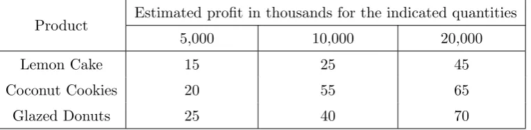
Example 3.1.1 A bakery usually sells the following three products, lemon cake, coconut cookies, or glazed donuts. Next year, the expected sales are highly uncertain, and

the owner decides to scale back to selling just one product. It is estimated that

profits will reflect the table below [Sha09].

Table 3.1: Products and Profits

Product Estimated profit in thousands for the indicated quantities

5,000 10,000 20,000

Lemon Cake 15 25 45

Coconut Cookies 20 55 65

Glazed Donuts 25 40 70

Which product should the bakery sell under the different criterion?

(a) Under the maximin criterion, we want to pick the best outcome from all of

the minimums. That is, if we only make five thousand of any product, the

best result will be the donuts. Thus, the bakery should make the donuts and

expect a $25,000 profit.

(b) The maximax is the best of the best, thus donuts will yield $70,000 profit if

the bakery makes 20,000 of them.

(c) If we use the Laplace method, where we assume that each outcome is just as

likely, we have for lemon cakes,

1 3(15) +

1 3(25) +

1

3(45) = 28.33.

For coconut cookies,

1 3(20) +

1 3(55) +

1

3(65) = 46.67.

And for glazed donuts,

1 3(25) +

1 3(40) +

1

(29)

Thus, under this criteria, the bakery should sell the cookies.

(d) Under the Hurwicz alpha criteria, assume α = 0.6, then for lemon cakes we

have,

0.6(45) + 15(1−0.6) = 33.

For coconut cookies,

0.6(65) + 20(1−0.6) = 47.

And for glazed donuts,

0.6(70) + 25(1−0.6) = 52.

Thus, the bakery should sell the donuts.

(e) For the regret criteria, we must subtract the highest possible pay-off under

each state of nature from the outcomes associated with each of the possible

events. From the opportunity loss table, we want to minimize future regret,

and as such, the bakery should choose to sell the coconut cookies.

Table 3.2: Opportunity Loss Table

Product 5,000 10,000 20,000 Max Regret

Lemon Cake (25-15)=10 (55-25)=30 (70-45)=25 30

Coconut Cookies (25-20)=5 (55-55)=0 (70-65)=5 5

Glazed Donuts (25-25)=0 (55-40)=15 (70-70)=0 15

It is important to note that a person cannot predict the outcome of any event,

by selecting an action we can expect some conclusions to occur which may be beneficial,

insignificant or even harmful. Thus, there is risk involved and in order to reach the

optimal decision we can use probability distributions out of the probable outcomes based

upon previously collected data. This is another type of decision making category which

we will call decision making underrisk. We can make our decisions according to a model

that will yield the largest expected profit value which is called expected money value

or EMV for short. EMV is used in order to calculate risk and facilitate the decision

making process. EMV is calculated with the following equation.

EM V(Ci) = n

X

i=1

(30)

Here,

Ci = Course of action i,

Pi = Probability of occurrence of outcomeO,

n= Number of possible outcomes,

Oi = The pay-off expected or outcome of actioni.

The equation above for EMV is another way of illustrating the expected value

of a probability distribution.

Example 3.1.2 A trading company is considering expansion. We need to determine whether to operate from an existing office and cover the area by traveling, or to

open a new locale closer to the new market. We come up with the following data:

[Sha09].

Table 3.3: Current vs. Expansion

Alternatives States of Nature Probability Pay-off

A. Operate from current office i) Increase in demand by 30% 60% 50

ii) No change 40% 5

B. Open new office i) Increase in demand by 30% 70% 40

ii) No change 30% -10

The expected pay-off forAis 0.6(50) + 0.4(5) = 32, and the expected pay-off forB

is 0.7(40) + 0.3(−10) = 25. As a result, we decide to stay at the current location and operate by trading locally and by traveling to the new market.

Decision making underconflict arises when there is more than one option open

for optimal gain, mainly due to the action of others in the field. This is where game

theory comes in handy. Some concepts that can be analyzed by game theory isexpected

value of perfect information or EVPI. This is the average outcome of the states of

nature of the level of information. That is to say, the information is available and the

probabilities are known and hence we can calculate the best option that results on the

highest profit possible. So EVPI = (best outcome of first state of nature)(probability of

first state of nature) + (best outcome of second state of nature)(probability of second

(31)

of nature). There is also the concept of expected profit with perfect information or

EPPI. EPPI is the maximum obtainable monetary gain given that all possible parameters

are known and accounted for. We can then define this relationship as

EV P I =EP P I−EM V,

where, EPPI is the expected profit with perfect information, and EMV is the expected

monetary value.

Example 3.1.3 As a manufacturer we want to increase our business. There are two choices available to choose from, first, expansion of the existing capacity at a cost

of 8 units, or second, modernization of current capacity at a cost of 5 units. We

estimate a 35% probability of having a high demand versus a 65% probability of

having no change on demand. Additionally, when demand is high, we will be

earning 12 units if we decide to expand, against 6 units if we decide to modernize.

If there is no change in demand, we will earn 7 units on expansion versus 5 units

for modernization. Let S1 be the state of nature pertaining to high demand with

probability P1 at 35%. Let S2 be the state of nature corresponding to no change

in demand with probability P2 at 65%. Also, list the courses of action as A1 for

expansion, and A2 for modernization. The conditional profits will be given by the

difference of the new revenue and the cost of expansion or modernization [Sha09].

Table 3.4: Conditional Profits

States of Nature A1 A2

S1 12−8 = 4 6−5 = 1

S2 7−8 =−1 5−5 = 0

Then, the expected monetary values are:

EM V(A1) = 4(0.35) + (−1)(0.65) = 0.75,

and

EM V(A2) = 1(0.35) + 0(0.65) = 0.35.

Thus we choose to expand since this course of action will maximize EMV. Now, we

need to calculate the EPPI by choosing the optimal course of action for each state

(32)

Table 3.5: Expected Profit with Perfect Information

States of Nature Probability Optimal Course of Action Expected Profit

S1 0.35 A1 4(0.35) = 1.4

S2 0.65 A2 0(0.65) = 0

Therefore EPPI is 1.4 + 0 = 1.4.

Hence,

EP P I−EM V =EV P I

1.4−0.75 = 0.65.

3.2

Decision Trees

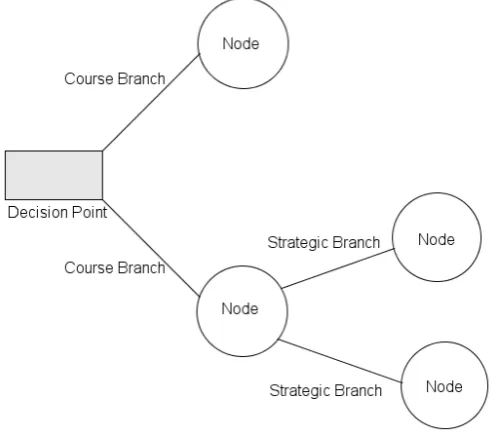
Decision making may involve multiple stages and at each stage, each decision will

open up different outcomes with their respective pay-offs. Adecision tree facilitates this

process. A decision tree is made up of nodes, branches, probabilities, and the resultant

pay-offs of each outcome. Decision trees are graphical tools that allows us to see how

decisions affect the outcomes.

(33)

Possibly the most important tool available to a decision maker is posterior

probabilities and analysis. By evaluating old decisions, new and improved models

can be derived. With new information, new alternatives can be considered . This may

drastically change future expected pay-offs. Bayes’ Theorem, is used to calculate the

effects and relationships of prior probability, the initial probability statement with

pay-offs, posterior probability, and allows us to revise probability statements due to post data

analysis.

Example 3.2.1 Suppose we are offered two investment opportunities, call them A and

B. The probability of success on A is 70% and on investment B is 40%. Both

investments require a capital of $2,000 to get started. InvestmentA returns $3,000

while investment B returns $5,000. If either investment fails, we lose our initial

capital of $2,000. We can only partake in one investment at a time. Thus, our

options are, to take investment A and stop, or if successful we may continue onto

investmentB. Or we may start with investmentBand stop, or if successful continue

with investmentA. Which is the best course of action? [Sha09].

We have the following courses of action:

i. Take A and stop.

ii. Take B and stop.

iii. Take A and if successful, takeB.

iv. Take B and if successful, takeA.

We begin by filling in the decision tree, shown on the next page, with the actual

investments values, and from there we can calculate the expected values of each

decision. For example, taking on investment A and succeeding gives a payout of

$3000, but if we fail, we will lose the capital investment of $2000. If we are successful

at A, we reach decision point 2. From here we can choose to stop, at which point

we will collect $3000, or we may continue with investment B. IfB is successful, we

collect the new pay-out of $5000 plus we still have the amount fromAfor a total of

$8000. However, if investment B fails, we lose $2000, but we still have $1000 from

the initial gain from A. The same logic follows if we decide to take investment B

(34)

Figure 3.2: Investment Opportunities.

on which investment we take first, the pay-out for failing on the second investment

will be different. Also, failing at any investment first carries the same negative

expectancy of −$2000. Thus, if we want maximum pay-out, we must follow the path that carries the greatest expected value for our choices.

The expected value ofAsucceeding and thenB succeeding is given by (8000)(0.6)+

(1000)(0.4) = 3800 Thus, $3800 is the expected value at decision point 2. The

expected value of taking only A is (3800)(0.7) + (−2000)(0.3) = 2060. Thus $2060 is the expected value of investment A succeeding alone.

If the investments are reversed, the expected value of B succeeding and then A

succeeding is given by (8000)(0.7) + (3000)(0.3) = 6500, which is the expected value

(35)

(−2000)(0.6) = 1400.

Although, success in both investments yields the same pay-out, which path should

we take? At decision point 1, we can compare the expected values of 2060 and 1400,

at which point we follow the largest which is to invest in A first. At this juncture,

the expected value of continuing versus stopping is 3800 versus 3000, so we decide

to continue with investmentB. This is the strategy offered in iii. Hence, takingA

and if successful taking B is the best course of action since it returns the greatest

(36)

Chapter 4

Theory of Games

4.1

Types of Games

Game theory comes into practice when there is a well understood problem and

the action of all persons of interest are known beforehand. For example, actions taken by

companyAwould have a direct impact on companyB, and thus companyBmust react to

the new situation, and must react optimally. Once companyB has adjusted, companyA

could readjust to the new environment and alter its own actions once again. Thus, game

theory is mainly used in figuring out the decisions and options given a set of conflicting

outputs and the motives of competing parties. Game theory applies when a game is finite,

that is, there exists a limited number of choices, and a finite number of moves at each

choice, and most importantly, each choice follows a rational set of rules and behaviors.

This will ensure that an acceptable outcome can be predefined for each game. Since game

theory deals with human thoughts, a player must take into account its environment. Each

player is an independent decision maker, but the outcome of the game would depend on

the action and strategies taken by all players. Since each player may have a different goal

in mind, this would be categorized as decision making under conflict. Players may

not all be motivated by maximum profit, but rather by optimal dominating decisions

over other players which may help in that particular player dominating the game in the

long run. Thus each player must be prepared with strategies and counter-strategies for

any given outcome. Game theory is then an interactive process that must be analyzed

(37)

decipher our opponents goals.

There are many types of games, but can be reduced to the following:

1. 2-Person Zero-Sum Game, a game where the gain of one player is the loss of the other.

2. 2-Person Non-Zero-Sum Game, a game where gain and loss are not equal, and thus

the outcome is not obvious.

3. N-Persons Game, a game where there exists a large number of players all trying to

maximize profits. There could be multiple winners, each with a different amount of

profit.

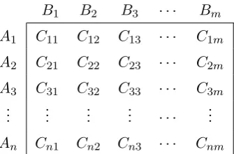
In order to represent a game with fixed strategies for two players, we can draw

a simple matrix like the next table below.

Table 4.1: Standard Matrix

B1 B2 B3 · · · Bm

A1 C11 C12 C13 · · · C1m

A2 C21 C22 C23 · · · C2m

A3 C31 C32 C33 · · · C3m ..

. ... ... ... · · · ...

An Cn1 Cn2 Cn3 · · · Cnm

The matrix indicates the expected pay-offs as values obtained from using

strat-egyAand strategyB. For example, if playerAadopts strategyA2and playerB counters

with strategy B3, then the resulting pay-off will beC23. It is standard practice to show

the pay-offs from the columns player, that is in this case, from player A’s perspective,

where positive numbers indicate gains and negative numbers indicate losses. For the

other player, these values would be reversed.

For the remainder of this chapter we focus on 2-person games in which Sharma

assumes the following rules:

1. Players act rationally and intelligently.

2. Each player has all relevant information.

3. Each player can use the information in a finite number of moves with finite choices for

(38)

4. Players make independent decisions of courses of actions without consultation.

5. Players play the game for optimization.

6. The pay-off is fixed and known in advanced.

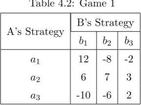
Example 4.1.1 Solve the game [Sha09].

Table 4.2: Game 1

A’s Strategy B’s Strategy

b1 b2 b3

a1 12 -8 -2

a2 6 7 3

a3 -10 -6 2

We want to find the optimal strategy pair for both playersAandB. PlayerAwants

to maximize his profits, while player B wants to minimize his losses. We can solve

the game by finding the maximin, the maximum of the minimums for playerA, and

the minimax, the minimum of the maximums for playerB. From the matrix we can

derive that the minimum for each of player A strategies is {-8, 3, -10}. From this set, player A will attempt to secure the maximum pay-off of 3. Similarly, player

B maximums from each of his strategies is the set {12, 7, 3} from which we must give up the minimum of 3. Thus, the solution to the game is given by the strategies

a2b3. In this game, by following the same strategy, playerA can gain 3 units from

player B. The solutiona2b3 is said to be optimal, since it is the only strategy that

will yield the safest return for player A, and at the same time, player B gives up

the least amount of equity. When a unique solution to a game exists, it is said to be

a saddle point. A saddle point is the point of equilibrium for both strategies. At

this point there exists a maximum gain for player A and minimum loss for player

B.

Let’s look at what the previous example solution means. Player A has three

strategies open to him. If he chooses either a1 or a3 he risks losing as indicated by the

negative numbers. Only a2 offers a profit every time, and at worst, player A can only

(39)

seem like the maximum pay-off, and thus the one that we should be striving to obtain,

we run the risk of losing -8 and -2 when player B chooses b2 and b3 respectively. Even

if we assume that each strategy is as likely to be chosen, by Laplace criterion we have

1 3(12) +

1

3(−8) + 1

3(−2) = 0.66, which makes choosing this strategy not ideal. Another

point to consider is, when playerBrealizes that playerAis constantly choosinga1, player

B can switch to playingb2 exclusively, and thus he will win 8 units from player Aevery

time.

By following the assumptions above, we can define astrategy as an alternative

course of action available to all players in advance. There are two types of strategies. A

pure strategy is where a player selects the same strategy each time without variation.

In this manner, each player knows exactly what the other player would do against his

own selected strategy. The other type of strategy is a mixed strategy. Here each of the

players use a combination of strategies, and each player leaves the other one guessing as

to what he would do next. Thus, opposing players must bring their own counter-strategy

with the aim of optimization. Regardless of which type of strategy is used, an optimal

strategy is the preferred course of action. Such a strategy will put the player in a superior

position regardless of his competitor’s actions. This will lead to the player obtaining a

maximum pay-off, a measurement of achievement, or a gain in profit. The pay-off as

previously discussed is the expected outcome, or the expected value, which we will call

the value of the game, which is obtained when players follow their optimal strategies.

2-Person zero-sum games can then be either purely strategic, where a players

follows one particular action to victory, or a mixed strategy game, where a players adapts

different strategies depending on the present situation. When both players use the best

strategy and said strategy is optimal, a saddle point exists. In Example 4.1.1, the saddle

point is a2b3 which has a value of 3.

4.2

Domination

A game with multiple strategies will lead to a large matrix. However, some

of those strategies could be dominated by another strategy, and thus the matrix can

be simplified until we obtain a more manageable, smaller matrix. This is what we will

term as the concept of dominance. Dominance occurs when one strategy is clearly

(40)

another strategy regardless of which counter-strategy is used against it, such a strategy

will dominate, and that strategy will be the preferred course of action to use. Domination

is applied as follows: [Sha09].

1. The rule of rows applies when all elements in a row are less than or equal to the

corresponding elements in another row. Such row is then said to be dominated and

can be removed from future play.

2. The rule of columns, applies when all elements in a column are greater than or equal to

the corresponding elements in another column. That column is said to be dominated

and can be removed from future play.

3. The rule of averages is when a pure strategy may well be dominated by the average of

two or more pure strategies. This will reduce the matrix faster since we can remove

several rows and, or columns simultaneously, if these are found to be dominated by

one of the previously mentioned rules.

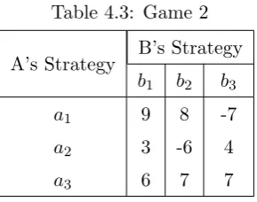
Example 4.2.1 Solve the game [Sha09].

Table 4.3: Game 2

b1 b2 b3

a1 9 8 -7

a2 3 -6 4

a3 6 7 7

Before we attempt to solve this game we should look for saddle points. If a saddle

point exists, then there exists a pure strategy available to both players. The

min-imums from each of A’s strategies is {-7, -6, 6} which has a maximum of 6. Now, the maximums from B are {9, 8, 7} whose minimum is 7. Since 66= 7, there is no saddle point, and a pure strategy does not exist. However, we may now turn our

attention to removing dominated strategies from the matrix. By the rule of rows

we can see that all values from a2 are less than those from a3. Thus we say that

a3 dominates a2. Player A will always achieve a better result by choosing a3 over

a2 regardless of what option playerB chooses. By removing a2 from the matrix we

(41)

Table 4.4: Game 2, Row Reduced

b1 b2 b3

a1 9 8 -7

a3 6 7 7

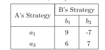
Now, by rule of columns, playerBcan removeb2since it is dominated byb3, because

values in b2 are greater than or equal to those inb3. Thus, the new reduced game

is given by the matrix as:

Table 4.5: Game 2, Row/Column Reduced

b1 b3

a1 9 -7

a3 6 7

PlayerAminimums from each strategy are{-7, 6}whose maximum is 6, and player

B maximums are {9, 7}whose minimum is 7. Since 66= 7, no pure strategy exists. Hence, player A must play a mixed strategy froma1 anda3, while player B reacts

by playing a mixed strategy fromb1andb3. It is important to note, that it could be

possible for a saddle point to appear once dominated strategies have been removed.

In the example above, both players must choose mixed strategies, but how often

should they play each strategy? Furthermore, why does player A not simply choose a3

as his sole strategy since he can at worst get 6 units from player B?

Perhaps it is not obvious from the preceding example, but playerA should still

play a1 from time to time, even at the risk of losing 7 units to player B. In order to

illustrate this point, we can look at a simplified game with all positive values.

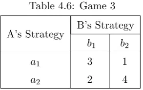
Example 4.2.2 In Game 3, playerA can choosea2 every time since this will secure him

at a minimum a pay-off of 2 units. Player B also loses the minimum by choosing

b1. However, playerAnotices that playerB always choosesb1, so playerAswitches

toa1 in order to get a better profit of 3. PlayerB follows the same argument and

(42)

Table 4.6: Game 3

b1 b2

a1 3 1

a2 2 4

they switch their strategies in order to maximize and minimize their respective

winnings and losses. Assuming playerAalternates between his two options equally,

his expected value from b1 is 1₂(3) + 1₂(2) = 2.5 which is preferable over strictly

choosing a2 which will only give him 2. Similarly, the expected value from b2 is 1

2(1) + 1

2(4) = 2.5. Thus player A must play a mixed strategy since his expected

value for both strategies is greater when using mixed strategies than by using a

pure strategy alone.

Is it possible that playerA can actually increase his expected value by playing

one strategy more than half the time, and if so, how often should he play each strategy?

Sharma provides three methods for solving games, algebraic, graphical, and linear

pro-gramming. For the purpose of this project we will focus on the algebraic method. The

algebraic method for solving a 2 by 2 game is derived by the following general formula:

Table 4.7: Algebraic 2 by 2 Matrix

B1 B2

A1 C11 C12

A2 C21 C22

Suppose playerAselects strategyA1 with probabilitypandA2 with probability

1−p. Suppose player B selects strategy B1 with probability q and B2 with probability

1−q. Then, the expected value of A versusB1 is

C11(p) +C21(1−p).

Now, using the values from Example 4.2.2 and the general formula, we can algebraically

(43)

plays against b1:

3(p) + 2(1−p) = 3p+ 2−2p

=p+ 2.

When playerA plays againstb2 we have:

1(p) + 4(1−p) =p+ 4−4p

=−3p+ 4.

The solution is given when these equations equal each other,

p+ 2 =−3p+ 4

4p= 2

p= 1 2.

How often should player A select each strategy? Since p = 1₂, player A must play a1

50% of the time, and he must balance his play by selecting a2 the other 50% of the time.

In this example it turns out that A can maximize his expected value by exactly playing

each strategy one half of the time! But this is not the case for B. When playerB plays

against a1 we have:

3(q) + 1(1−q) = 3q+ 1−q

= 2q+ 1.

And when B plays againsta2 we have:

2(q) + 4(1−q) = 2q+ 4−4q

=−2q+ 4.

The solution is given when these equations equal each other,

2q+ 1 =−2q+ 4

4q = 3

(44)

In order for playerB to minimize his losses, he must playb1 75% of the time, andb2 the

remaining 25% of the time.

We can now revisit Example 4.2.1, Game 2, to find out how often each player

must play each strategy. We have, A’s strategy versus b1 as 9(p) + 6(1−p) and versus

b3 as −7(p) + 7(1−p). Solving these equations and setting them equal to each other

gives p= ₁₇1 . Similarly, forB we have, againsta1, 9(q) + (−7)(1−q) and againsta3 we

have 6(q) + 7(1−q). Solving these equations and setting them equal to each other obtain

q = 14₁₇. Thus, in Game 2, player A must play a mixed strategy that contains a1 1/17

of the time, a2 zero percent of the time (since it is dominated), and a3 the remaining

16/17 of the time. Player B must play b1 14/17 of the time, b2 zero percent of the time

(since it is also dominated), and b3 the remaining 3/17 of the time. The expected value

for the game from playerA’s perspective is 9(₁₇1 ) + 6(1− 1 17) =

105

17. And from playerB’s

perspective 9(14₁₇)−7(1−14 17) =

105

17. Hence, by using the mixed strategies above, playerA

stands to win approximately 6.18 units while player B stands to lose the same amount.

Thus, this is the optimal strategy for each player to follow.

As stated earlier, when dealing with game theory, we are assuming that the gain

of one player is the loss of another player. However, it is highly unlikely that a player

will have access to all of the required information ahead of time. The lack of information

will leave us guessing as to whether a specific strategy is optimal or not. Therefore,

we must restrict our assumptions to a basic standard set of rules that are well defined

and understood by all players. In real life, competitors will not divulge their strategies,

and as such, pay-offs will not be known, which implies that courses of actions cannot

be predicted. Thus, a decision maker is left with the option of taking risk since the

outcomes are uncertain. Furthermore in real life, there could be more than two players,

(45)

Chapter 5

Poker Models

5.1

Uniform Poker Models

We now turn our attention to solving poker models. These are simplified poker

games that can be solved algebraically. We will now assume that we are playing

two-person zero-sum games. The participants will be called player 1 and player 2. In this type

of game, a player will gain some amount from the other player, and this sum will always

be zero. We will also assume that hands are randomly and independently distributed.

For the models, player 1 is dealt a random hand X ∈ [0,1] where X has a uniform distribution over the interval [0,1]. To be precise, of all minimum and maximum values

for each member of the family, all intervals of the same length on the distribution have

equal probabilities. In this case, in a standard deck of 52 cards, the probability of getting

dealt one specific card is exactly 1/52, the probability of getting dealt a second specific

card is exactly 1/51, and so on. Getting dealt a specific card does not influence the

outcome of the second card. Similarly, player 2 is also dealt an independently random

hand Y ∈ [0,1] with equal uniform distribution on [0,1] as X. Both players are well aware of the value of their own hands, but have no information on their opponent’s hand

strength. We can think of it as each player has a number between 0 and 1, but they

have no idea if their opponent’s number is higher or lower. On each model there exists a

betting structure. Both players must pay a “unit” worth, (decided amongst the players

in advance) that is paid before the hands are dealt, this is called anante. The antes and

(46)

and bets. Each player will have a predefined set of actions available to them. Player

1 may decide to bet or not to bet his hand, and player 2 reacts with his own actions,

whether to call or fold. For all models we are ignoring other options found in poker,

which could be for player 1 to check-raise, check-call, or for player 2 to bet his own hand

or to raise when faced with a bet by player 1, amongst some common poker strategies.

At the end of the game, the hands are compared at what is know asshowdown, and the

highest valued hand wins the pot.

If we disregard the randomly distributed hands, given that players’ options

are known and announced, will make this game a game of perfect information. This

type of game can be solved using one or more techniques as described in the previous

chapters about decision analysis and game theory. However, since we are ignorant of our

opponent’s holdings, this is then called a game of almost perfect information, where

we may deduce the strength of our opponent’s cards by what we have. For instance, if I

have an ace it is less likely that my opponent has an ace of his own, or, since I hold two

spades, it is less likely that my opponent has any spades at all. Thus, we may study and

derive the correct strategy to play using decision trees which we will be calling betting

trees.

5.2

Borel’s Poker

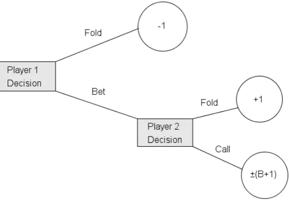
Borel’s poker model is referred to as La Relance (Figure 5.1). In this model

each player pays one unit in ante and then they are dealt their respective randomly

independent uniformly distributed hands. Player 1 acting first, will have two options,

one tofold his hand, that is, to discard one’s hand and forfeit interest in the current pot.

In this case, player 1 surrenders the hand to player 2, giving up his claim to the pot, and

conceding the pot to player 2. When player 1 folds, he loses his ante, and player 2 wins

one unit. The second option is for player 1 to make a wager, to bet some valueB where

B > 0 and B may not necessarily be equal to an ante’s worth but could be higher. In

the case that player 1 bets, if player 2 folds, then player 1 wins the two antes, and gains

one unit worth. If player 2 calls the bet, then hands are compared at showdown, and the

best hand will take the pot and in this case will gain both antes, plus whatever the betB

was, for a net worth of B+ 1 ante. The model disregards the case where both hands are

(47)

Figure 5.1: La Relance.

when dealing with real cards, as opposed to random number distributions, such cases do

occur in real life. In such a scenario, both bets are returned and there is no exchange

of money between the players. Borel’s poker game favors player 2, given that player 1

must decide to either bet or fold, puts him at a starting disadvantage, he will bet with

his strong hands and will only lose to a better hand with a small probability, but at the

same time he will not get called often by a worse holding. As a result, player 1 will only

gain just the ante [FF03].

The following result is attributed to Borel.

Borel’s Theorem: The value of La Relance is:

V(B) =− B

2

(B+ 2)2.

The unique optimal strategy for player 2 is to call if Y > c and to fold otherwise,

where

c= B

B+ 2

An optimal strategy for player 1 is to bet if X > c2 and to fold otherwise.

Showing that these strategies are optimal can be done using the principle of

(48)

Players can choose either course of action without affecting the overall value of the game.

Suppose then, that player 2 chooses the point c in such a way as to make player 1

indifferent between folding and betting. If player 1 bets with a hand whereX < che will

win 2 units when Y < c (since player 2 is playing optimally and he will fold), and will

lose B when player 2 has a handY > c. Player 1 will have a handX > csome percent of

the time, the remaining time his hand will be in the interval 1−c. Now, if player 1 folds, he will win nothing. Player 1 is then indifferent at the point c when 2c−B(1−c) = 0. Then,

2c−B(1−c) = 0

2c−B+BC= 0

2c+BC=B

c(2 +B) =B

c= B

B+ 2.

Example 5.2.1 Suppose two players play with $1 antes and $5 bets, who does this game favor by Borel’s Theorem?

The value of the game is

V(5) =− 5

2

(5 + 2)2 =−

25

49 =−0.51.

Since the game is shown from player 1’s perspective, and the value of the game is

negative, this game favors player 2. With these specific antes and bets, player 1

will lose 51 cents on average, that is, the expected value for player 1 is−$0.51.

In the game above, as stated before, player 1 starts at a disadvantage. By the

rules of the game, player 1 must choose whether to bet or to fold his hand. The pot

consists of $2 worth of antes, and player 1 must risk $5 in order to win $1, since he

will only gain his opponent’s ante. If player 2 calls, player 1 stands to win $6 from his

opponent, but if he loses, player 1 will lose his $1 ante plus his $5 bet. Player 1 has the

option to fold at the beginning of the game, giving up his ante to player 2, which means

he still loses $1. Regardless of how much the antes and the bets are worth, the value of

the game for player 1 is always negative, thus, this is a game that we should not play as

(49)

bet if X > c2, or to fold otherwise. So whenB = 5

c= B

B+ 2 = 5

7 = 0.71.

Then

c2 = (5₇)2 = 25

49 = 0.51.

The optimal strategy for player 2 is to call ifY > c= 0.71 and to fold otherwise.

Let’s take a closer look at the implications that these numbers have on our game. Player

1 will receive a hand from the interval [0,1], if his number is lower than 0.51 he will fold

automatically, losing his ante to player 2. Now, there will be many instances when player

2’s number is less than 0.51, if we assume equal distribution, 51% of the time it will be

lower and 49% of the time it will be higher.

For an extreme example, suppose player 1 draws a 0.50, he has to fold to player

2, even knowing that player 2 will have half of the time a number even lower than 0.50.

Now, if player 1 draws a number higher than 0.51 he will bet, and now player 2 must call if

and only if his own number is greater than 0.71. Thus player 1 will still lose, say when he

draws anything between 0.52 and 0.71, but also when both players have numbers greater

than 0.72 but player 2’s number is gr

THINKING POKER THROUGH GAME THEORY

CSUSB ScholarWorks

Table of Contents

List of Tables

List of Figures

Chapter 1

Chapter 2

Distributions and Expected Value

Enumeration

Variance

Bayes’ Theorem

Chapter 3

Decision Trees

Chapter 4

Domination

Chapter 5

Borel’s Poker