Reverse Evolution of Armor Plates in Threespine Stickleback
Jun Kitano,1 Daniel I. Bolnick,2 David A. Beauchamp,3 Michael M. Mazur,3 Seiichi Mori,4
Takanori Nakano,5 and Catherine L. Peichel1,*
1Division of Human Biology, Fred Hutchinson Cancer Research Center, Seattle, Washington
98109
2Section of Integrative Biology, University of Texas, Austin, Texas 78712
3U.S. Geological Survey, Washington Cooperative Fish & Wildlife Research Unit, School of
Aquatic and Fisheries Sciences, University of Washington, Seattle, Washington 98105
4Biological Laboratory, Gifu-keizai University, Ogaki, Gifu 503-8550, Japan
5Research Department, Research Institute for Humanity and Nature, 335 Takashima-cho,
Kamigyo-ku, Kyoto 602-0878, Japan
*Correspondence: Catherine L. Peichel; phone: (206) 667-1628; fax: (206) 667-2917; email:
Summary
Faced with sudden environmental changes, animals must either adapt to novel environments, or
go extinct. Thus, studying the mechanisms underlying rapid adaptation is not only crucial for
understanding natural evolutionary processes, but also for understanding human-induced
evolutionary change, an increasingly important problem [1-8]. In the present study, we
demonstrate that the frequency of completely-plated threespine stickleback fish (Gasterosteus
aculeatus) has increased in an urban freshwater lake (Lake Washington, Seattle, Washington)
within the last 40 years. This is a dramatic example of “reverse evolution” [9] because the
general evolutionary trajectory is towards armor plate reduction in freshwater sticklebacks [10].
Based on our genetic studies and simulations, we propose that the most likely cause of reverse
evolution is increased selection for the completely-plated morph, which we suggest may result
from higher levels of trout predation after a sudden increase in water transparency during the
early 1970s. Rapid evolution was facilitated by the existence of standing allelic variation in
Ectodysplasin (Eda), the gene that underlies the major plate morph locus [11]. The Lake
Washington stickleback thus provides a novel example of reverse evolution, likely caused by a
Results and Discussion
Reverse Evolution of Armor Plates in Lake Washington
The threespine stickleback (Gasterosteus aculeatus) is a good model system for elucidating the
ecological and genetic mechanisms underlying phenotypic evolution [12-13]. One dramatic and
prevalent phenotypic change in these fish is the reduction of armor plates covering the lateral
body surface that occurred repeatedly after freshwater colonization 12,000 years ago [10]. While
ancestral marine sticklebacks typicallyhave a continuous row of lateral plates (completely-plated
morph), freshwater sticklebacks usually have a reduction in lateral plates, resulting in a gap in
the middle part of the plate row (partially-plated morph) or loss of both the middle and posterior
plates (low-plated morph). The major gene responsible for reduction of the stickleback lateral
plates across the world is Ectodysplasin (Eda) [11]. There are two major alleles of Eda found in
stickleback populations, here referred to as the complete allele and the low allele. Most marine
sticklebacks are homozygous for the complete allele, although marine sticklebacks that are
heterozygous carriers of the low allele are found at a low frequency [11]. It is proposed that
when marine sticklebacks colonize freshwater environments, strong selection results in an
increase in the frequency of the low Eda allele, leading to the prevalence of low-plated fish in
In contrast to the prevalence of the low-plated morph in many freshwater environments
[10, 11], we found a high frequency of completely-plated stickleback in Lake Washington, an
urban freshwater lake in Seattle [14-16]. In 2005, we found all three lateral plate morphs were
present, with 49% complete morphs, 35% partial morphs, and 16% low morphs (Figures 1A and
2C). Although a previous study had also shown that all three morphs were present in Lake
Washington in 1968/1969, only 6% were classified as complete morphs (Figure 1A; [17]).
Instead, the low morph, with a mode of seven plates, was the most common morph until the late
1960s (Figures 1B and C). In 1976, bimodal peaks appeared, one corresponding to fish with
seven plates and another corresponding to fish with 32 plates (Figure 1C; [18]). The frequency of
fish with 33 plates was even higher in the 2005 sample (Figure 1C). The increase in completely
plated fish in the 2005 sample did not reflect bias in the sampling methods (n = 322, χ2 = 6.6949,
df = 4, p = 0.1529) or the seasonal (Figure S1) or geographical (Figure 2C) distribution of
differently plated sticklebacks. These data demonstrate that the frequency of plate morph
phenotypes has changed dramatically in Lake Washington within the past 40 years, which is
equivalent to 40 generations in this stickleback population [18].
Genotyping of the 2005 samples at the Eda locus revealed a strong association
< 10-47; Figure S2; Table S1). By ANOVA, the Eda genotype explains 75.2% of the variance in
plate number in the Lake Washington stickleback. This is close to the percent of phenotypic
variance in plate number explained by the Eda locus in laboratory crosses (76.9 %; [19]). Thus,
the increase in the completely plated phenotype in Lake Washington is likely due to an increase
in the frequency of the Eda complete allele, given the previously established link between plate
phenotype and Eda genotype in stickleback populations across the world [11].
Gene Flow is Not the Primary Cause of Armor Plate Evolution in Lake Washington
Most marine sticklebacks in Puget Sound are completely plated (Figure 2C), with high
frequencies of the complete Eda allele (Figure 2D). Because marine sticklebacks can now
migrate into the lake through the Lake Washington Ship Canal (Figures 2B and S3), which was
built in 1917 [14], an increase in migration may have contributed to the increase of lateral plates
in the Lake Washington stickleback. In order to test this hypothesis, we collected sticklebacks in
neighboring marine environments (Puget Sound), multiple points in Lake Washington, and in
neighboring streams (Figure 2) and genotyped them with 15 microsatellite markers (Table S2).
Genetic data were then analyzed with the Bayesian clustering software STRUCTURE [20].
genetic clusters (K) was three (Figure S4). Estimation of ancestry for each individual revealed
that the stickleback in Lake Washington have two main genetic sources (Figure 2E). Stickleback
sampled from near the ship canal were genetically similar to marine stickleback (indicated by
green in Figure 2E), while those sampled close to the streams were more similar to neighboring
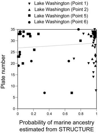
stream stickleback (indicated by blue in Figure 2E). However, there was no significant
correlation between the probability of marine ancestry and plate number (Pearson correlation r =
0.005, p = 0.967; Figure S5). Multidimensional scaling of the genetic distance matrix also
confirmed the lack of association between genotypes at neutral loci and plate number (Figure S6).
Thus, the increase in armor plates in Lake Washington does not result simply from the presence
of marine sticklebacks in the lake.
It may be still possible that an increase in long-term migration from Puget Sound has
contributed to the overall increase in the complete morph in the lake. To test this possibility, we
first estimated migration rates (m; fraction of migrants per generation) from the genetic data and
then examined whether the empirically estimated m can explain the observed plate evolution. We
used both Isolation with Migration (IM) and LAMARC software [21-23] to estimate the m
between a Lake Washington population and a Puget Sound marine population (Table S3). The m
(LAMARC), while the m from Lake Washington into Puget Sound was estimated as 6.43 x 10⁻⁴
(IM) or 1.20 x 10⁻³ (LAMARC). Then, we developed deterministic numerical simulations to
calculate the m required for the observed change of plate phenotype under different selection
regimes (Figure S7). In the absence of selection (s = 0), migration would need to be 0.148 to
explain the observed change from 1969 to 1976 and 0.035 to explain the change from 1969 to
2005. These values are inconsistent with our low (m < 10-3) migration rate estimates, suggesting
that there was a period of selection that favored the complete morph in Lake Washington.
Changes in Selection Regime in Lake Washington
By using the empirically estimated values of m, we found that a selection coefficient s (strength
of selection for the complete morph) of 0.58-0.72 (Table 1) can explain the evolutionary shift
from 1969 to 1976 (from 6% complete morphs to 40.2% complete morphs; Figure 1A). This
suggests that the complete morph had 58-72 % higher fitness than the low morph during this
period. To explain the transition between 1976 and 2005 (from 40.2% complete morphs to 49%
complete morphs), s of 0.01-0.03 is required (Table 1). We thus conclude that there was a period
of very intense selection for the complete morph between 1970 and 1976, followed by a
One of the dramatic ecological changes that occurred in Lake Washington during the
early 1970s is increased water transparency due to the mitigation of eutrophication in the late
1960s. Water transparency in the lake was 1-2 m Secchi depth (the maximum depth at which a
white Secchi disk is visible from the water surface) during 1955-1971, and increased to 3.4 m in
1973 and then to 6-7 m from 1976 to the present [14, 15]. Previous behavioral experiments have
demonstrated that an increase in water transparency significantly increases the reaction distance
of visual predators to their prey, thus leading to increased predation pressure on prey fish [24].
Cutthroat trout (Oncorhynchus clarki) are visual predators, extremely sensitive to subtle changes
in water transparency [24], and the primary predator of threespine stickleback in both the littoral
and pelagic zones of Lake Washington [16, 25, 26]. Therefore, we used a visual foraging model,
which calculates the search volume by cutthroat trout as a function of light intensity and turbidity
[27, 28], to investigate a possible change in stickleback predation regime. This analysis
demonstrated that the increase in lake transparency created an 8-fold increase in the visual search
volume by cutthroat trout and also expanded the depth range over which effective visual foraging
could occur (Figure 3). Most of the expanded search volume was achieved during 1972-1975,
when the mean Secchi disk transparency increased to 3.4 m. Although the cutthroat trout
suggests that an increase in lake transparency could have changed the predation regime by
increasing encounter rates between stickleback and cutthroat trout.
Predation by toothed predators, such as cutthroat trout, is thought to favor
completely-plated stickleback because the posterior lateral plates can protect the stickleback
from being injured and swallowed [29, 30]. Reimchen predicted that the complete morph would
occur in open water habitats of high clarity where capture rather than pursuit defenses
predominate [29]. Consistent with this hypothesis, we have shown that the increase in the
frequency of complete morphs occurred during the time when the water clarity increased
dramatically in Lake Washington, a relatively deep and large lake (a surface area of 8.76 x 10⁷
m2 and a maximum depth of 65.2 m). Further supporting the hypothesis that an increase in
predation by cutthroat trout has contributed to the rapid evolution of Lake Washington
stickleback, recent stickleback samples are larger than historical stickleback samples (Figure 1B;
Table S4). Larger body size can protect against predation by gape-limited predators, such as
cutthroat trout [31, 32]. Although salinity and water temperature have also been proposed as
factors contributing to lateral plate evolution [33, 34], we can exclude a role for these abiotic
Conclusions
We have reported a dramatic example of “reverse evolution” [9], in which there has been an
increase in completely-plated sticklebacks in a freshwater lake. Our data demonstrate that
selection for the complete morph was particularly strong during the early 1970s, suggesting that
the main increase in the frequency of completely plated fish may have occurred in less than a
decade. Armor reduction has also been shown to occur within only a few decades after the
introduction of marine sticklebacks into freshwater [35-37]. Thus, sticklebacks can respond to
environmental changes by either an increase or a decrease in lateral plates within a few decades.
Rapid phenotypic evolution in stickleback provides us a great opportunity to further investigate
the mechanisms by which animals can respond to rapidly changing environments [38].
The rapid evolution of armor plates in Lake Washington sticklebacks may have been
enabled by the presence of standing genetic variation at the major plate locus [11]. Without
standing variation, a sudden increase in predation may have led to population extinction before a
new mutation appeared [6, 39]. Although an increase in gene flow was not the primary cause of
armor evolution, gene flow from the marine population may have enabled rapid armor evolution
by contributing to standing genetic variation within the lake [7, 40]. This work provides an
been proposed as a major mechanism of contemporary evolution [4, 8]. Thus, investigating the
genetic mechanisms that underlie adaptive phenotypes is essential for a better understanding of
rapid evolutionary change [2, 4, 8, 41].
Although we suggest that reverse evolution in the Lake Washington stickleback is
likely attributable to the change in water clarity, we still lack direct evidence for this hypothesis
and additional factors may have also contributed. As in many other cases of rapid evolution [5],
it is often difficult to tease apart all the potential factors that contribute to phenotypic evolution.
We demonstrated, however, that changes in water clarity are able to influence predator-prey
interactions; further attention should be given to the influence of water clarity on predator-prey
interactions and animal evolution. In addition, this work highlights the importance of
investigating the relationships between environmental changes, species interactions, and the
genetic basis of phenotypic evolution, both to better understand the mechanisms of animal
evolution and inform conservation efforts.
Supplemental Data
Detailed experimental procedures, a supplemental discussion, eight figures and five tables are
Acknowledgements
This work was supported by a Uehara Memorial Fellowship (JK), the Packard Foundation (DIB),
Seattle Public Utilities (DAB), Water and People Project (SM), and a Burroughs Wellcome Fund
Career Award in the Biomedical Sciences (CLP). Sampling was conducted under Washington
Department of Fish and Wildlife permits to CLP (05-049, 06-159, 07-047) and DAB (06-115),
and an ESA Section 10a permit #1376 from NOAA to DAB. All experiments were approved by
Institutional Animal Care and Use Committees (FHCRC IACUC #1575; UW IACUC #3286-01).
We thank D. Schluter, D. Kingsley, J. Gow, and B. Stein for comments on the manuscript, K.
Maslenikov and T.W. Pietsch for access to the University of Washington Fish Collection,
Seabeck Conference Center for access to their pond, Z. Baldwin, T. Kobayashi, T. Akimichi, J.
Wittouck and N. Hurtado for technical assistance, and T.P. Quinn, P. Westley, F. Goetz, L.
Gilbertson, W. Aron, T. Flagg, D. Maynard, Y. Kitano, C. Sergeant, N. Overman, A. Bruner, A.
Wark, P. Pagels, members of the Peichel and Beauchamp labs, and many field assistants for
discussions and sampling assistance.
References
Change (New York: W.W. Norton & Company).
2. Smith, T.B., and Bernatchez, L. (2008). Evolutionary change in human-altered
environments. Mol. Ecol. 17, 1-8.
3. Carroll, S.P., Hendry, A.P., Reznick, D.N., and Fox C.W. (2007). Evolution on
ecological time-scales. Funct. Ecol. 21, 387-393.
4. Hendry, A.P., Ferrugia, T.J., and Kinnison, M.T. (2008). Human influences on rates of
phenotypic change in wild animal populations. Mol. Ecol. 17, 20-29.
5. Majerus, M. (1998). Melanism: Evolution in Action (Oxford: Oxford University Press).
6. Reznick, D.N., Ghalambor, C.K., and Crooks, K. (2008). Experimental studies of
evolution in guppies: a model for understanding the evolutionary consequences of
predator removal in natural communities. Mol. Ecol. 17, 97-107.
7. Stockwell, C.A., Hendry, A.P., and Kinnison, M.T. (2003). Contemporary evolution
meets conservation biology. Trends. Ecol. Evol. 18, 94-101.
8. Gienapp, P., Teplitsky, C., Alho, J.S., Mills, J.A., and Merila, J. (2008). Climate change
and evolution: disentangling environmental and genetic responses. Mol. Ecol. 17,
167-178.
Org. Evolution 55, 653-660.
10. Bell, M.A., and Foster, S.A. (1994). The Evolutionary Biology of the Threespine
Stickleback (Oxford: Oxford University Press).
11. Colosimo, P.F., Hosemann, K.E., Balabhadra, S., Villarreal, G., Dickson, M., Grimwood,
J., Schmutz, J., Myers, R.M., Schluter, D., and Kingsley, D.M. (2005). Widespread
parallel evolution in sticklebacks by repeated fixation of Ectodysplasin alleles. Science
307, 1928-1933.
12. Kingsley, D.M., and Peichel, C.L. (2007). The molecular genetics of evolutionary change
in sticklebacks. In Biology of the Three-Spined Stickleback, S. Östlund-Nilsson, I. Mayer,
and F.A. Huntingford, eds (Boca Raton: CRC press), pp 41-81.
13. Schluter, D. (2000). The Ecology of Adaptive Radiation (New York: Oxford University
Press).
14. Edmondson, W.T. (1991). The Uses of Ecology: Lake Washington and Beyond (Seattle:
University of Washington Press).
15. Edmondson, W.T. (1970). Phosphorus, nitrogen, and algae in Lake Washington after
diversion of sewage. Science 160, 690-691.
size-related foraging of wild cutthroat trout in Lake Washington. Northwest Sci. 66,
149-159.
17. Hagen, D.W., and Gilbertson, L.G. (1972). Geographic variation and environmental
selection in Gasterosteus aculeatus L. in the Pacific Northwest, America. Evolution Int. J.
Org. Evolution 26, 32-51.
18. Dykeman, R.G. (1980). An investigation of the young of the year and age I fish
population in southern Lake Washington. University of Washington masters thesis.
19. Colosimo, P.F., Peichel, C.L., Nereng, K., Blackman, B.K., Shapiro, M.D., Schluter, D.,
and Kingsley, D.M. (2004). The genetic architecture of parallel armor plate reduction in
threespine sticklebacks. PLoS Biol. 2, 635-641.
20. Pritchard, J.K., Stephens, M., and Donnelly, P. (2000). Inference of population structure
using multilocus genotype data. Genetics 155, 945-959.
21. Beerli, P., and Felsenstein, J. (1999). Maximum-likelihood estimation of migration rates
and effective population numbers in two populations using a coalescent approach.
Genetics 152, 763-773.
22. Nielsen, R., and Wakeley, J. (2001). Distinguishing migration from isolation: a Markov
23. Kuhner, M.K. (2006). LAMARC 2.0: maximum likelihood and Bayesian estimation of
population parameters. Bioinformatics 22, 768-770.
24. Mazur, M.M., and Beauchamp, D.A. (2003). A comparison of visual prey detection
among species of piscivorous salmonids: effects of light and low turbidities. Env. Biol.
Fish. 67, 397-405.
25. Nowak, G.M., Tabor, R.A., Fresh, K.L., and Quinn, T.P. (2004). Ontogenetic shifts in
habitat and diet of cutthroat trout in Lake Washington, Washington. North Am. J. Fish.
Mang. 24, 624-635.
26. Beauchamp, D.A. (1994). Spatial and temporal dynamics of piscivory: implications for
food web stability and the transparency of Lake Washington. Lake Reserv. Manag. 9,
151-154.
27. Beauchamp, D.A., Baldwin, C.M., Vogel, J.L., and Gubala, C.P. (1999). Estimating diel,
depth-specific foraging with a visual encounter rate model for pelagic piscivores. Can. J.
Fish. Aquat. Sci. 56 (Suppl. 1), 128-139.
28. Mazur, M.M., and Beauchamp, D.A. (2006). Linking piscivory to spatial-temporal
distributions of pelagic prey fishes with a visual foraging model. J. Fish Biol. 69,
29. Reimchen, T.E. (1992). Injuries on sticklebacks from attacks by a toothed predator
(Oncorhyncus) and implications for the evolution of lateral plates. Evolution Int. J. Org.
Evolution 46, 1224-1230.
30. Reimchen, T.E. (2000). Predator handling failures of lateral plate morphs in Gasterosteus
aculeatus: implications for stasis and distribution of the ancestral plate condition.
Behaviour 137, 1081-1096.
31. Reimchen, T.E. (1991). Trout foraging failures and the evolution of body size in
stickleback. Copeia 1991, 1098-1104.
32. Moodie, G.E.E. (1972). Predation, natural selection and adaptation in an unusual
threespine stickleback. Heredity 28, 155-167.
33. Heuts, M.J. (1947). Experimental studies on adaptive evolution in Gasterosteus aculeatus
L. Evolution Int. J. Org. Evolution 1, 89-102.
34. Hagen, D.W., and Moodie, G.E.E. (1982). Polymorphism for plate morphs in
Gasterosteus aculeatus on the east coast of Canada and an hypothesis for their global
distribution. Can. J. Zool. 60, 1032-1042.
35. Bell, M.A., Aguirre, W.E., and Buck, N.J. (2004). Twelve years of contemporary armor
814-824.
36. Klepaker, T. (1993). Morphological changes in a marine population of threespine
stickleback, Gasterosteus aculeatus, recently isolated in freshwater. Can. J. Zool. 71,
1251-1258.
37. Kristjánsson, B.K., Skúlason, S., and Noakes, D.L.G. (2002). Rapid divergence in a
recently isolated population of threespine stickleback (Gasterosteus aculeatus). Evol.
Ecol. Res. 4, 659-672.
38. Reimchen, T.E, and Nosil, P. (2002). Temporal variation in divergent selection on spine
number in threespine stickleback. Evolution Int. J. Org. Evolution 56, 2472-2483.
39. Barrett, R.D.H., and Schluter, D. (2008). Adaptation from standing genetic variation.
Trends Ecol. Evol. 23, 38-44.
40. Garant, D., Forde, S.E., and Hendry, A.P. (2007). The multifarious effects of dispersal
and gene flow on contemporary adaptation. Funct. Ecol. 21, 434-443.
41. True, J.R. (2003). Insect melanism: the molecules matter. Trends Ecol. Evol. 18,
Figure Legends
Figure 1. Lateral Plate Evolution in Lake Washington Stickleback
(A) Temporal change in the frequency of the completely (black bar), partially (gray bar), and low
(white bar) plated morphs in Lake Washington stickleback. Sample sizes are shown above the
graph. Right panels show representative images of the three morphs in stickleback. Skeletal
structures are visualized by alizarin red staining. Scale bars = 10 mm.
(B) Representative images of stickleback collected in March 1957 and March 2006 in the
northern pelagic zone of Lake Washington by midwater trawling.
(C) Histograms of lateral plate number for stickleback collected in 1957, 1968/1969, 1976, and
2005. Sample sizes are the same as in Figure 1A. The most common plate number is also shown
in each panel as a mode. Among stickleback collected in 1968/1969, 22% had more than 12
plates, but the individual plate counts for each fish are not available [17]. Plate number was
counted from the left side of the fish except in the 1976 sample, for which only right plate
number data were available [18]. For the 1957 data, museum specimens in the University of
Washington Fish Collection were analyzed. The frequency of morph was significantly different
between successive sampling time points (χ2- test; p < 0.05) except between 1957 and 1968/1969
Figure 2. Genetic and Morphological Variation around Lake Washington
(A) Map of Washington State. Blue dots indicate the collection sites of marine stickleback from
Puget Sound. Lake Washington is highlighted by a square and magnified in Figure 2B.
(B) Map of Lake Washington and neighboring streams. Numbers indicate the sampling sites in
Lake Washington: Point 1, Union Bay; Point 2, northern pelagic zone (Area 1 in [17]); Point 3,
Matthews Beach; Point 4, Tracy Owen Park; Point 5, Juanita Beach; Point 6, Yarrow Bay; Point
7, Mercer Slough; Point 8, east channel; Point 9, northern pelagic zone (Area 2 in [17]).
(C) Variation in plate morph frequencies among populations. Each column indicates the
frequency of the complete (black bar), partial (gray bar), and low (white bar) morph stickleback
for each population. Numbers in parentheses indicate sample size. The frequency of different
morphs was not significantly different among different points within Lake Washington (n = 322,
χ2 = 17.0, d.f. = 14, p = 0.255).
(D) Variation in the allele frequency of Eda among populations. The black bar indicates the
frequency of the complete Eda allele and the white bar indicates the frequency of the low Eda
allele at Stn382. Numbers in parentheses indicate sample size.
(E) Genetic structure of sticklebacks collected in Lake Washington, Puget Sound and
individual is represented by a thin column that is partitioned into colored segments indicating the
estimated proportion of ancestry from each cluster. Numbers in parentheses indicate sample size.
Figure 3. Changes in Cutthroat Trout Foraging Volume in Lake Washington.
(A-C) Depth-specific search volumes of cutthroat trout are shown during peak eutrophication in
1955-1971 (A), initial recovery during 1972-1975 (B), and the current transparency regime
1976-2006 (C). Different diel periods are indicated with white bars for day, hatched bars for
dusk, and black bars for night.
(D) Changes in the search volume by trout are shown as the percentage of the current search
volume. Black and white circles indicate the search volumes at the depths of 0-60 m and 10-20 m,
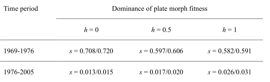
Table 1. Estimation of Strength of Selection (s) for the Complete Plate Morph.
Dominance of plate morph fitness Time period
h = 0 h = 0.5 h = 1
1969-1976 s = 0.708/0.720 s = 0.597/0.606 s = 0.582/0.591
1976-2005 s = 0.013/0.015 s = 0.017/0.020 s = 0.026/0.031
Values of s during different time periods were calculated for different values of the dominance of
plate morph fitness (h). Migration rates estimated by LAMARC (left side in each cell) and IM
(right side in each cell) were used. Frequencies of 6%, 40.2%, and 49.0% complete plate morphs
Supplemental Data
Experimental Procedures
Morphological Analysis
All 2005-2007 samples were collected between March and June by minnow trap and mid-water
trawling, except for samples from Points 8 and 9 (Figure 2B), which were collected by purse
seining in October 2005 and mid-water trawling in September 2006, respectively. The 1957
sample was collected by Dr. William Aron in the northern pelagic zone of the lake in March by
mid-water trawling (University of Washington fish collection No. UW 012691). Plate numbers
for the 1968/1969 and 1976 samples were taken from [S1] and [S2], respectively. The 1968/1969
sample was collected at Points 4-6 (Figure 2B) between April and June by beach seining [S1].
The 1976 sample was collected from the southern end of the lake throughout the year by beach
seining and dip nets [S2]. For the 1957 museum samples and the 2005-2007 samples, plate
number was counted under a dissecting microscope from the left side of the fish stained with
alizarin red as previously described [S3]. All fish analyzed were larger than 32mm standard
length, at which point plate development is complete [S4]. Fish were assigned to one of three
Genetic Analysis
DNA isolation and microsatellite analyses were conducted as previously described [S3], except
that the reactions were analyzed on an ABI 3100 (Applied Biosystems, Foster City CA) and
visualized with ABI GeneMapper 3.7 (Applied Biosystems, Foster City CA). For genotyping the
Eda locus, fish were genotyped with the Stn382 microsatellite marker located in the first intron
of the Eda gene [S5]: the complete and low alleles gave rise to 218 bp and 158 bp bands,
respectively. For population genetic studies, fish were genotyped with 15 microsatellite markers
chosen using a random number table. These markers are on 14 different linkage groups (LG) and
have allele size distributions consistent with the stepwise mutation model (Table S2). These data
were first analyzed with STRUCTURE [S6], which uses Markov chain Monte Carlo simulations
to find groupings that minimize Hardy-Weinberg and linkage disequilibrium within cluster
groups. Since Stn46 and Stn238 are both on LG4, linkage information was included in the input
file for STRUCTURE analysis, although no significant linkages were indicated between any
markers within each sampling site (exact test [S7], p > 0.05, after Bonferroni correction). We
estimated the number of clusters in the data by running three simulations for each K value from
K = 1 through K = 10 to calculate the mean log probability of data (L(K)), and using the ad hoc
Parameters were estimated after 200,000 iterations, following a burn-in of 25,000 iterations.
For estimation of migration rates, we analyzed the genetic data from the Duwamish
marine (n = 21) and Lake Washington (Point 1; n = 27) sticklebacks with both IM and
LAMARC software [S10-S12]. Using all Lake Washington stickleback populations for the
LAMARC estimation gave rise to similar results (not shown). For calculation of m and Ne, we
used a mutation rate of 10-4, as previously described [S13]. We ran LAMARC with 10 short
chains of 1,000 samples and 2 long chains of 20,000 samples. IM results were based on
recording of 30,000,000 steps after 100,000 of burn-in. In both IM and LAMARC, multiple runs
gave rise to similar results.
The pairwise genetic distance (Dps) between individuals from Lake Washington, Puget
Sound, and nearby streams was calculated from the proportion of shared alleles using MSA
software [S14]. Then, the genetic distance matrix was subject to principal coordinate (PCo)
analysis using the R statistical package. The correlations between the first and second PCo and
plate number were tested by a Pearson correlation test.
Estimating the Strength of Selection
locus, such that complete morphs had genotype 218 bp/218 bp; partial morphs were 218 bp/158
bp, and low morphs were 158 bp/158 bp. Given the initial frequency of low morphs in
1968/1969, f(L) = 0.7, we estimated the initial frequency of allele 158 to be q = 0.837. This was
used to calculate the frequency of complete and partial morphs assuming Hardy-Weinberg
equilibrium. Given initial frequencies of the three morphs, f(C), f(P), and f(L), we next calculated
the frequencies of these morphs following selection:
w L f L f w hs P f P f w s C f C f ) ( )' ( ) 1 )( ( )' ( ) 1 )( ( )' ( = + = + =
where s is the strength of selection for or against complete plate morphs, h determines the
dominance of plate morph fitness, and w =1+sf(C)+hsf(P). Assuming selection acts on
stickleback armor phenotypes throughout development, followed by immigration of adults prior
to breeding, we then calculated the effects of migration following selection:
) ( )' ( ) 1 ( ' )' ( ) ( )' ( ) 1 ( ' )' ( ) ( )' ( ) 1 ( ' )' ( mar mar mar L mf L f m L f P mf P f m P f C mf C f m C f + ! = + ! = + ! =
where m is the fraction of individuals in Lake Washington who immigrated from marine
Washington population, so reverse migration does not appreciably affect marine population
frequencies and we can adopt a continent-island model. Following a round of selection and
migration, we calculated new allele frequencies, and determined the morph frequencies assuming
random mating and Hardy-Weinberg equilibrium. Numerical iterations led to estimates of the
final morph frequencies after a specified period of time, for a given starting morph frequency.
We then iteratively used a large number of parameter combinations (s, h, and m) to determine the
s necessary for a given observed change assuming a particular heritability and migration rate, or
the m required for the same change assuming no selection.
Visual Foraging Model
We used a visual foraging model [S15-S17] for predatory cutthroat trout feeding in the pelagic
regions of the lake during thermally-stratified periods when most predation on fish was measured
[S18]. The model estimated search volumes SV (m3) at any depth during any diel period, based
on changes in reaction distance RD (m) of predators to forage fishes as functions of light
intensity I (Lux) and turbidity T (NTU), swimming speed SS (m/hr), and the duration D (hr) of
each diel period (Table S5):
Where for T ≤ 1 NTU
RD = 0.337 I0.118 (I < 17 Lux)
or
RD = 0.5316 (I ≥ 17 Lux).
For T > 1 NTU
RD = 0.337 I0.118 T-0.624 (I < 17 Lux)
or
RD = 0.5316 T-0.624 (I ≥ 17 Lux).
Depth-specific search volumes were computed for each diel period at 5-m depth intervals using
incident light levels I0 and light extinction coefficients k and turbidity levels from each of the
lake transparency regimes (1955-1971: Secchi depth transparency = 1-2 m; 1972-1975: Secchi
depths = 3.4 m; 1976-2006: Secchi depths = 6-7 m; Table S5). Depth-specific light levels Iz were
computed for each depth z (m):
Iz = I0 ekz.
Turbidity values were only available during 2002-2003 [S17], so values for earlier transparency
regimes were estimated from a regression of Secchi depths (m) versus turbidity (r2 = 0.73; p =
T = 4.58 – 0.475 Secchi.
Because light extinction increases with declining transparency, we also attempted to compute an
average light extinction coefficient for the 1955-1971 period using a regression of Secchi depth
versus k (r2 = 0.49; p = 0.122; n = 6):
k = -0.708 + 0.051 Secchi;
however, the nonsignificant regression created some uncertainty regarding the accuracy of k =
-0.63 estimated for the peak eutrophication period. To examine the sensitivity of our analysis to k,
we compared the search volume estimates using the regression estimate of k = -0.63 versus k =
-0.35, the current high-transparency value. When using the high transparency value for k, the
adjusted search volume during the 1955-1971 period only increased from 12% to 20% of the
current search volume. This result implies that in the unlikely event that no change in light
extinction accompanied the improved water transparency, current predation pressure might have
only increased 5-fold instead of 8-fold following peak eutrophication. Thus any error in our light
extinction estimate would result in a modest change in the magnitude the predation increase, but
would not change the overall conclusion that predation pressure increased markedly between the
Sr Isotope Analysis
Sr stable isotope analysis of calcified fish tissues can tell us their migratory history, because
different water bodies usually have different 87Sr/86Sr ratios [S19]. In order to investigate the
presence of direct migrants from Puget Sound, threespine sticklebacks were collected in the ship
canal above the Chittenden Locks in May 2007 with minnow traps and preserved in ethanol after
euthanasia. Sr analysis was conducted as described previously with several modifications [S20].
Seven to 50 mg of fish vertebrae was surgically taken and dissolved in a 15mL Teflon vessel by
adding 2mL of 68% ultrapure-grade HNO3. Upon complete dissolution, the resulting solution
was dried and suspended with a few drops of 1N HCl. Ten to 20 mL of water sample were
filtered through a cellulose acetate filter (pore size 0.2 µm), transferred to a 30 mL Teflon vessel,
and dried on a hot plate. Sr was separated and isolated using classical cation exchange
chromatography using AG50WX-12 resin (Muromachi Technos, Tokyo, Japan) with distilled 2N
and 6N HCl as elution solution. The concentrations of Sr isotopes were determined using a
thermal ionization mass spectrometer (Triton, Thermo Fisher Sci., Yokohama, Japan) at the
Research Institute for Humanity and Nature. The 87Sr/86Sr ratio of nine standard samples of
normalized to the recommended 87Sr/86Sr ratio of 0.710250.
Supplemental Discussion
Because the current salinity (0-0.1 ppt) of Lake Washington has not changed significantly over
the last 50 years [S1, S21], the rapid increase in armor plates in Lake Washington stickleback
cannot be attributed to changes in salinity [S22, S23]. Although the water temperature of the lake
has risen, possibly due to global warming [S24], higher water temperatures are usually
associated with the presence of the low plate morph [S22, S23], suggesting that a change in
water temperature is not the likely cause of rapid armor evolution.
Supplemental References
S1. Hagen, D.W., and Gilbertson, L.G. (1972). Geographic variation and environmental
selection in Gasterosteus aculeatus L. in the Pacific Northwest, America. Evolution Int. J.
Org. Evolution 26, 32-51.
S2. Dykeman, R.G. (1980). An investigation of the young of the year and age I fish
population in southern Lake Washington. University of Washington masters thesis.
Schluter, D., and Kingsley, D.M. (2001). The genetic architecture of divergence between
threespine stickleback species. Nature 414, 901-905.
S4. Bell, M.A., Aguirre, W.E., and Buck, N.J. (2004). Twelve years of contemporary armor
evolution in a threespine stickleback population. Evolution Int. J. Org. Evolution 58,
814-824.
S5. Colosimo, P.F., Hosemann, K.E., Balabhadra, S., Villarreal, G., Dickson, M., Grimwood,
J., Schmutz, J., Myers, R.M., Schluter, D., and Kingsley, D.M. (2005). Widespread
parallel evolution in sticklebacks by repeated fixation of Ectodysplasin alleles. Science
307, 1928-1933.
S6. Pritchard, J.K., Stephens, M., and Donnelly, P. (2000). Inference of population structure
using multilocus genotype data. Genetics 155, 945-959.
S7. Raymond, M., and Rousset, F. (1995). GENEPOP (version 1.2): population genetics
software for exact tests and ecumenicism. J. Hered. 86, 248-249.
S8. Evanno, G., Regnaut, S., and Goudet, J. (2005). Detecting the number of clusters of
individuals using the software STRUCTURE: a simulation study. Mol. Ecol. 14,
2611-2620.
populations of sympatric threespine sticklebacks. J. Evol. Biol. 20, 2173-2180.
S10. Beerli, P., and Felsenstein, J. (1999). Maximum-likelihood estimation of migration rates
and effective population numbers in two populations using a coalescent approach.
Genetics 152, 763-773.
S11. Nielsen, R., and Wakeley, J. (2001). Distinguishing migration from isolation: a Markov
chain Monte Carlo approach. Genetics 158, 885-896.
S12. Kuhner, M.K. (2006). LAMARC 2.0: maximum likelihood and Bayesian estimation of
population parameters. Bioinformatics 22, 768-770.
S13. Kitano, J., Mori, S., and Peichel C.L. (2007). Phenotypic divergence and reproductive
isolation between sympatric forms of Japanese threespine stickleback. Biol. J. Linn. Soc.
91, 671-685.
S14. Dieringer, D., and Schlötterer, C. (2003). Microsatellite analyzer (MSA): a platform
independent analysis tool for large microsatellite data sets. Mol. Ecol. Notes 3, 167-169.
S15. Mazur, M.M., and Beauchamp, D.A. (2003). A comparison of visual prey detection
among species of piscivorous salmonids: effects of light and low turbidities. Env. Biol.
Fish. 67, 397-405.
depth-specific foraging with a visual encounter rate model for pelagic piscivores. Can. J.
Fish. Aquat. Sci. 56 (Suppl. 1), 128-139.
S17. Mazur, M.M., and Beauchamp, D.A. (2006). Linking piscivory to spatial-temporal
distributions of pelagic prey fishes with a visual foraging model. J. Fish Biol. 69,
151-175.
S18. Beauchamp, D.A., Vecht, S.A., and Thomas, G.L. (1992). Temporal, spatial, and
size-related foraging of wild cutthroat trout in Lake Washington. Northwest Sci. 66,
149-159.
S19. Kennedy, P.K., Klaue, A., Blum, J.D., Folt, C.L., and Nislow, K.H. (2002).
Reconstructing the lives of fish Sr isotopes in otoliths. Can. J. Fish. Aquat. Sci. 59,
925-929.
S20. Nakano, T., Tayasu, I., Wada, E., Igeta, A., Hyodo, F., and Miura, Y. (2005). Sulfur and
strontium isotope geochemistry of tributary rivers of Lake Biwa: implications for human
impact on the decadal change of lake water quality. Sci. Total Environ. 345, 1-12.
S21. Edmondson, W.T. (1991). The Uses of Ecology: Lake Washington and Beyond (Seattle:
University of Washington Press).
L. Evolution Int. J. Org. Evolution 1, 89-102.
S23. Hagen, D.W., and Moodie, G.E.E. (1982). Polymorphism for plate morphs in
Gasterosteus aculeatus on the east coast of Canada and an hypothesis for their global
distribution. Can. J. Zool. 60, 1032-1042.
S24. Arhonditsis, G.B., and Brett, M.T. (2004). Effects of climatic variability on the thermal
Figure S1. Seasonal Variation in Lateral Plate Phenotype
We analyzed stickleback collected in April-June 2005 from littoral zones (Points 1, 3-7; n = 186),
October 2005 from the east channel (Point 8; n = 40), March 2006 from Area 1 of the northern
pelagic zone (Point 2; n = 40), April-June 2006 from littoral zones (Points 1 and 5; n = 46),
September 2006 from Area 2 of the northern pelagic zone (Point 9; n = 61), and May 2007 from
Figure S2.Association between Eda Genotype and Lateral Plate Number
Histograms of plate number are shown for the Lake Washington stickleback that are
homozygous for the complete allele (218bp allele) (upper panel; n = 79), homozygous for the
low allele (158bp allele) (lower panel; n = 32), and heterozygous for the complete allele and low
allele (middle panel; n = 85), at the Stn382 locus. Means (and 95% confidence intervals) of plate
number for the 218/218, 218/158, and 158/158 genotypes are 32.58 (31.60-33.56), 26.00
(25.02-26.9), and 10.00 (8.46-11.54). Stickleback collected from Point 1 (n = 67), Point 2 (n =
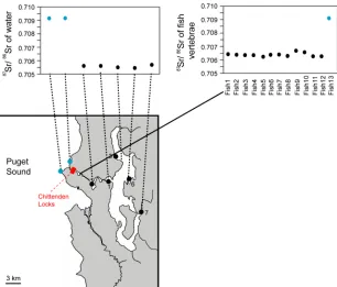
Figure S3. Identification of Migrants by Sr Isotope Analysis
Water was collected from different places and subjected to Sr isotope analysis (left panel), which
revealed that the 87Sr/86Sr ratio is higher in seawater (blue circles) than lake water (black circles).
Sr isotope analysis of the vertebrae of stickleback collected in the ship canal above the
Chittenden Locks (right panel) revealed that one fish (blue circle) had a high 87Sr/86Sr and is
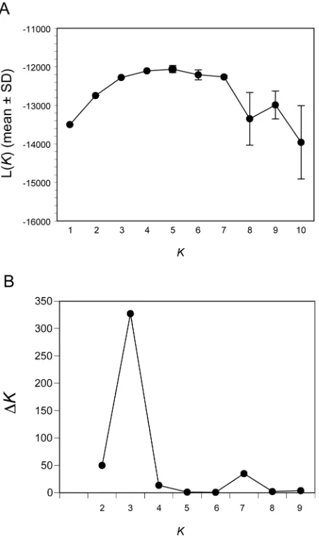
Figure S4. Estimation of Genetic Cluster Number with STRUCTURE
(A) Mean ± S.D. of the log probability of data L(K) for three simulations is shown for K = 1
through K =10. L(K) begins to plateau at K = 3 or 4.
(B) The ad hoc statistic ΔK has a unimodal peak at K = 3, suggesting that three is the most
Figure S5. Lack of Correlation between Plate Number and the Probability of Marine Ancestry
Figure S6. Multidimensional Scaling of Genetic Distance Matrix
(A) Scatterplot between the first (PCo1) and the second principal coordinate scores (PCo2) of the
genetic distance matrix based on neutral microsatellite loci for Lake Washington, Puget Sound,
and neighboring stream sticklebacks.
(B) Scatterplot between PCo1 and plate number (left panel) and between PCo2 and plate number
There is no significant association between plate number and genotypes at neutral microsatellite
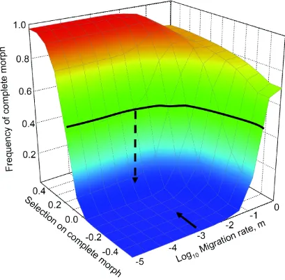
Figure S7. Contribution of Selection and Migration to Plate Evolution.
The expected frequency of completely plated morphs in Lake Washington in 2005 is plotted as a
function of selection for or against the completely plated morph, and the rate of immigration
from a marine population. The thick dark line represents the combination of migration rates and
(h = 0, 0.5, or 1), primarily in elevation of the curve surface (not shown). To illustrate the process
of estimating selection strength, we show a solid arrow representing an empirical estimate of the
migration rate (the LAMARC estimate of m = 1.77 x 10⁻³). One then finds the corresponding
selection strength that yields the empirically observed evolutionary change (vertical dashed
Figure S8. Cutthroat Trout Catch Rates in Lake Washington.
The mean (± 2SE) catch for all sizes of cutthroat trout per 24-hour set in benthic littoral gill nets,
and the mean (± 2SE) catch of large (FL ≥ 300 mm) cutthroat trout per purse seine set has not