Transmission Efficiency in Complex-Shaped Waveguide using Real Metals

(1)

Transmission E

ﬃ

ciency in Complex-Shaped Waveguide using

Real Metals

∗

)

Yoshihisa FUJITA

1)

_{, Soichiro IKUNO}

2)

_{and Hiroaki NAKAMURA}

1,3)

1)_{Depertment of Energy Engineering and Science, Nagoya University, 322-6 Oroshi, Toki, Gifu 509-5292, Japan}

2)_{Tokyo University of Technology, 1404-1 Katakura, Hachioji, Tokyo 192-0982, Japan}

3)_{National Institute for Fusion Science, 322-6 Oroshi, Toki, Gifu 509-5292, Japan}

(Received 10 December 2013/Accepted 23 March 2014)

The two-dimentional meshless time-domain method (2D-MTDM) was used to simulate the electromagnetic wave propagation phenomena in complex-shaped waveguides considering the inﬂuence of metals and to numer-ically investigate the relation of the dispersion medium with the attenuation rate. The simulation results suggest that the waveguide with grooves is strongly aﬀected by the frequency of the propagating wave than the waveguide without grooves because the wave propagating in the waveguide with the grooves penetrates deep into the metal compared with the waveguide without grooves. The transmission loss for the curved waveguide is greater than that for the straight waveguide.

c

2014 The Japan Society of Plasma Science and Nuclear Fusion Research

Keywords: millimeter wave, MTDM, dispersive media, Drude model, RC method DOI: 10.1585/pfr.9.3401074

1. Introduction

In the Large Helical Device (LHD), plasma is heated using the resonance of the millimeter waves. The millime-ter waves propagate on a long transmission path that bends several times. In the waveguides without grooves, trans-mission loss occurs because of the eddy currents induced into the metal constructing the waveguide. Thus, for ef-ﬁcient heating, it is necessary to reduce the transmission loss in the path.

For the transmission of millimeter waves, corrugated waveguides are used [1]. The transmission eﬃciency of the corrugated waveguides has been investigated [2–4]. The waveguide walls are assumed metallic, and the perfect electric conductor (PEC) was adopted as the boundary con-ditions to implement this assumption. However, the Joule heat was not generated because PEC has no electroresis-tance. In fact, theoretically, there is no energy loss if the PEC is adopted. The Drude model supports the complex dielectric constant required for the metals to be used as the waveguide walls [5].

The purpose of this paper is to develop a two-dimentional meshless time-domain mathod (2D-MTDM) code on the basis of the Drude model and the recursive convolution (RC) method. In addition, the inﬂuence of the dispersion metal and the grooves on the transmission ef-ﬁciency is investigated by calculating the electromagnetic wave propagation in the corrugated waveguide.

author’s e-mail: [email protected]

∗)_{This article is based on the presentation at the 23rd International Toki}

Conference (ITC23).

2. Numerical Method

Generally, the ﬁnite diﬀerence time domain method (FDTD) is used to analyze electromagnetic wave propaga-tion. However, the analytic domain must be divided into orthogonal meshes if FDTD is used for the simulations. In this paper, the MTDM is adopted to study the propagation of electromagnetic waves in complex domains. In addi-tion, the Drude model is adopted by the RC method for the dispersion model.

2.1 Meshless time-domain method

The governing equations for the two-dimensional wave propagation phenomena are deﬁned by following equations:

∂E

∂t =−

σ

εE+

1

ε∇ ×H, (1)

∂H

∂t =−

1

μ∇ ×E. (2)

Here,Edenotes the electric ﬁeld andHdenotes the mag-netic ﬁeld. Moreover,ε, μ, and σ denote the permittiv-ity, permeabilpermittiv-ity, and electroconductivpermittiv-ity, respectively. As mentioned above, the basic concept of MTDM is the same as that of FDTD. The time domain is discretized by the leapfrog algorithm. On the other hand, the space is dis-cretized by the shape functions obtained with the meshless method. To this end, the nodes, r1, r2, · · ·, and rN, are

scattered in the analytical domain and are on the bound-aries. Subsequently, we consider an arbitrary functionu(r). The value of the functionu(r) on node ri isui. Then, the

functionu(r) is interpolated by the shape functionsφi(r) as c

2014 The Japan Society of Plasma

(2)

follows: ˆ u(r)=

N

i₌1

uiφi(r). (3)

Here, ˆu(r) denotes the interpolation function ofu(r), and

φi(r) denotes the shape function corresponding to the node

ri. In this paper, we adopted the shape functions obtained

by the radial point interpolation method (RPIM) because a shape function satisﬁes the Kronecker delta function prop-erty [6]:

φi(rj)=δi j. (4)

By the above property, the values of the interpolation func-tion on the nodes are

ˆ u(rj)=

N

i₌1

uiφi(rj)= N

i₌1

aiδi j=uj. (5)

Note that the nodes for the electric and magnetic ﬁelds are scattered separately, as shown in Fig. 2. Thus, the shape functionsφeandφhare built from the nodes for the electric and magnetic ﬁelds, respectively [7]. By usingφe_and_φh_,

the electric ﬁeldEand the magnetic ﬁeldHare expressed by the shape functions as

ˆ En(r)=

Ne

k=1

Enkφek(r), (6)

ˆ Hn(r)=

Nh

l=1

Hn_lφh_l(r). (7) Here, the superscriptn denotes the number of time steps. In the MTDM, E(r) = (Ex(r),Ey(r),Ez(r)), H(r) =

(Hx(r),Hy(r),Hz(r)), and each components (x,y, andz) of

the electric ﬁeldEand the magnetic ﬁeld His present in the same position. In this paper, 2D-TM mode is adopted for the evaluation: r = (x,y), E(r) = (0,0,Ez(r)), and

H(r)=(Hx(r),Hy(r),0).

En_z_,_k= 1−α 1+αE

n₋1 z,k

+ Δt/ε

1+α

Nh

l=1

Hn−

1 2 y,l

∂φh l

∂x(rk)

− Δt/ε

1+α

Nh

l₌1

Hn−

1 2 x_,l

∂φh l

∂y(rk), (8)

Hn+

1 2 x,l =H

n−1 2 x,l −

Δt

μ

Ne

k=1

Enz_,k

∂φe k

∂y(rl), (9)

Hn+12 y,l =H

n−1 2 y,l +

Δt

μ

Ne

k=1

En_z_,_k∂φ

e k

∂x(rl). (10)

Here,Δtdenotes the computation time step and should sat-isfy the Courant condition. For the delta function property of Eq. (4), the values of the interpolation function on the nodes would be ˆEn

z(rk)=Enz_,k; the same applies to the

mag-netic ﬁeld and other components. In addition, the summa-tion is required in the case of using the partial derivative of

shape functions that are obtained by RPIM, because they do not satisfy the Kronecker delta function property [6]. Parameterαis deﬁned as follows:

α= σΔt

2ε . (11)

In MTDM,EandHare calculated using Eqs. (8), (9), and (10) at each time step, respectively.

2.2 Dispersion model

In the Drude model, the permittivity depends on the frequency of the propagating wave. Thus, the electric ﬂux density in the frequency-space ¯Dis deﬁned by the follow-ing equation in the dispersion medium:

¯

D(ω)=ε¯(ω) ¯E(ω). (12) Here,ωdenotes the angular frequency of the input wave, and the overline denotes the frequency-space function. Ap-plying the inverse Fourier transform to Eq. (12), the time-space function is obtained as follows:

D(t)= t

0

ε(τ)E(t−τ)dτ. (13)

Here, all electromagnetic fields are zero for negative time, because the input field is induced att=0. The past values of the electric field are stored to calculate Eq. (13) by the integral convolution. In this paper, the RC method is used to reduce the storage cost. In the Drude model, the relative permittivity ¯εr(ω) is defined by

¯

εr(ω)=1+

ω2 p

iω γ−ω2, (14)

where ωp denotes the plasma frequency and γ denotes

the inverse of the relaxation time. The Drude model is achieved using the RC method, and the electric ﬁeld is up-dated using the following equation:

Enz_,k=

1 1+χ0E

n−1 z_,k +

1 1+χ0ψ

n−1 z (rk)

+Δt/ε0

1+χ0 Nh

l₌1

Hn−

1 2 y_,l

∂φh l

∂x(rk)

−Δt/ε0

1+χ0 Nh

l=1

Hn−

1 2 x,l

∂φh l

∂y(rk). (15)

Here,ε0denotes the permittivity in vacuum. The

convolu-tion summaconvolu-tionψn−1

z (ri) and the initial value of the relative

electric susceptibility χ0 _{are deﬁned by following}

equa-tions

ψn₋1 z,k =E

n₋1 z,k Δχ

0₊_e−γΔt_ψn₋2

z,k , (16)

ψ0

z_,k=0, (17)

χ0₌ω

2 p

γ2

γΔt−1+e−γΔt. (18)

Moreover,Δχ0_{is deﬁned as}

Δχ0₌₋ω 2 p

γ2

(3)

The magnetic ﬁeld is assumed to be frequency indepen-dent. Therefore, the magnetic ﬁeld is updated by Eqs. (9) and (10).

3. Numerical Evaluation

The effects of the dispersion metal and grooves on the attenuation rate using the 2D-MTDM with the Drude model are investigated. Two types of analytical models are used. The models are shown in Fig. 1. The perfectly matched layer (PML) is adopted for absorbing the bound-ary conditions on the progressive wave direction [8], and the perfect electric conductor (PEC) is adopted for the boundary conditions of the analysis area. The values of the geometrical parameters used are as follows: The width of the waveguide is 2b+2d+w, the length of the straight waveguide is 15λ, the length of the curved waveguide is 5λ, the curvature radius of the curved waveguide is 5.25λ, b = 0.5λ,w = λ, p = 0.5λ,a = 0.25λ, andd = 0.25λ, whereλdenotes the wavelength of the input wave. Fur-thermore, the node alignment of the electric and the mag-netic fields is shown in Fig. 2. The value of the attenuation rate “RA” used in this paper is defined by the following

Fig. 1 Conceptual diagrams of the corrugated waveguide: (a) straight waveguide and (b) right-angle waveguide.

Fig. 2 Conceptual diagram of the nodes alignment in the waveg-uide.

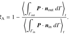
equation:

RA=1−

Γout

P·noutdΓ

t

Γin

P·nindΓ

t

. (20)

Here,Pdenotes the Poynting vector, nin denotes the

nor-mal vector ofΓin,nout denotes the normal vector ofΓout,

and the values of the attenuation rateRAare evaluated

us-ing the values on the source input lineΓinand the

observa-tion lineΓout. Moreover, the bracketftdenotes the time

average of f. The physical parameters used in this paper are the amplitude of the source wave (1 V/m), the wave speed (3×108m/s), the distance of the neighboring node (λ/40), the plasma frequency of aluminum ωp (2.8 PHz)

[5], the collision frequency of aluminum (12 THz) [5], the number of layers for PML (24), the dimension of PML (4), and the reﬂection factor of PML (−120 dB). Besides, the value ofEzis used as the input wave with the equation

Ez(rin,t)=β1

β2sin(ωt), ωt<8π,

sin(ωt), ωt≥8π. (21) Here,rin ∈Γs, andβ1andβ2are deﬁned by the following

equations:

β1=sin

rx,in−(b+d)

w π

, (22)

β2=

1 2

1−cos _ω_t

8

. (23)

The following equation is adopted for the radial basis func-tionF(|r|).

F(|r|)=|r|2+R2−0.5. (24) Here, the value of the support radiusRis 2lmin, wherelmin

denotes the minimum distance between the nodes. First, it was varified if the Drude model was embedded correctly. The value of the reflection rate when the plane wave is vertically generated against the dispersive wall is plotted as a function of the input wave frequency in Fig. 3. We can see from this figure that the reflection rate is cal-culated with high precision because the analytical solution and the simulation results are almost identical. In addition, the reflection rate is reduced when the frequency of the in-put wave is greater than the plasma frequency.

Second, the inﬂuence of the grooves on the attenuation rate in the straight waveguide is investigated. The values of the attenuation rateRAare plotted as a function of the

input wave frequency in Fig. 4. We see from this ﬁgure that the values of the attenuation rate are changing irregularly because the waves penetrate into the metal forω/ωp >1.

In addition, the attenuation rate is negative because the de-nominator of Eq. (20) increases for waves at approximately

Γinthat penetrate deeply into the metal compared to those

(4)

Fig. 3 Reﬂection rate of the plane wave. The wave is vertically generated against the dispersive wall.

Fig. 4 The values of attenuation rateRAplotted as a function of

input wave frequency in the straight waveguide.

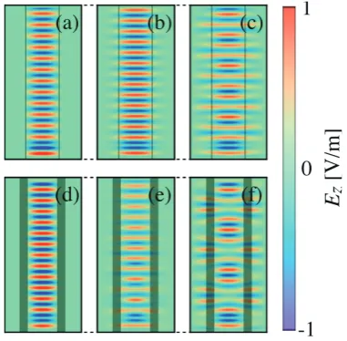
Fig. 5 Distribution of the electric ﬁeldEzin the straight

waveg-uide. The gray background indicates the area of the cor-rugated groove, or the boundary of the vacuum and the metal. (a), (b), and (c) without groove, (d), (e), and (f) with groove, (a), (d)ω/ωp=0.1, (b), (e)ω/ωp =1, and (c), (f)ω/ωp=3.

the distributions of the waveguide with grooves and with-out grooves forω/ωp =0.1 (see Figs. 5 (a) and 5 (d)). In

the waveguide without grooves, periodic distribution is

ob-Fig. 6 Distribution of the electric ﬁeldEz in the curved

waveg-uide without groove. The gray background is the bound-ary of the vacuum and the metal. ω/ωp =1, (a)w=3λ and the curvature radius is 15.75λand (b)w=λand the curvature radius is 5.25λ.

Fig. 7 The values of attenuation rateRAplotted as a function of

the input wave frequency in the curved waveguide.

tained (see Fig. 5 (b)), although a distorted waveform is ob-served forω/ωp>1 (see Fig. 5 (c)). On the other hand, we

can see from Figs. 5 (e) and 5 (f) that the distorted wave-forms are observed even ifω/ωp > 1; this is induced by

the corrugated waveguide.

Next, we investigate the inﬂuence of the width of the curved waveguide without grooves on the electromagnetic wave propagation as a run-up to evaluate the attenuation rate. The distribution of the electric ﬁeldEzin the

waveg-uide is shown in Fig. 6 for ω/ωp = 1. In the case of

w = 3λ(see Fig. 6 (a)), the incident wave is reﬂected on the waveguide wall. On the other hand, the wave propa-gates while maintaining the waveform in the case ofw=λ (see Fig. 6 (b)). This is due to the larger cutoﬀfrequency owing to the narrowing width of the waveguide.

Finally, we evaluate the values of attenuation rateRA

in the curved waveguide. The attenuation rateRAis

plot-ted as the function of the corrugaplot-ted channels in the curved waveguide (see Fig. 7). The distributions of the electric ﬁeldEzin the waveguide is shown in Fig. 8. From Figs. 7

(5)

Fig. 8 Distribution of the electric ﬁeldEzin the curved

waveg-uide. The gray background denotes the area of the cor-rugated groove or the boundary of the vacuum and the metal. (a), (b), and (c) without groove, (d), (e), and (f) with groove, (a), (d)ω/ωp=0.1, (b), (e)ω/ωp =1, and (c), (f)ω/ωp=3.

waveguide. In addition, the transmission loss of the curved waveguide is greater than that of the straight waveguide because the incident wave is reﬂected on the waveguide wall.

4. Conclusion

We have developed a numerical code for analyzing

the electromagnetic wave propagation in complex-shaped waveguide. In addition, we have evaluated the inﬂuence of the dispersion metal on the attenuation rate. The conclu-sions are summarized as follows:

1. In the case of the curved waveguide without grooves, the wave was propagated along the narrow width of the waveguide because the cutoﬀ frequency in-creased.

2. In both the straight and curved waveguides, the wave propagating in the waveguide with the grooves pene-trated deep into the metal compared with the waveg-uide without grooves.

3. The transmission loss for the curved waveguide was greater than in the case of the straight waveguide be-cause the incident wave was reﬂected on the waveg-uide walls.

Acknowledgment

This work is supported by KAKENHI (24656560). The authors wishes to thank Dr. A. Takayama for the help-ful discussions.

[1] M. Fujiwaraet al., J. Fusion Energy15, 7 (1996). [2] Y. Fujitaet al., J. Plasma Fusion Res.8, 2401061 (2013). [3] N. Kashimaet al., Jpn. J. Appl. Phys.52, 11ND02 (2013). [4] H. Nakamuraet al., J. Phys.: Conf. Ser.410, 012046 (2013). [5] R.D. Radicet al., Appl. Opt.37, 22, 5271 (1998).

[6] G.R. Liuet al., Comput. Mech.36, 421 (2005).

[7] T. Kaufmannet al., IEEE Trans. Microw. Theory Tech.58, 3399 (2010).