118
COMBINING ARTIFICIAL NEURAL NETWORK- GENETIC ALGORITHM AND
RESPONSE SURFACE METHOD TO PREDICT WASTE GENERATION AND
OPTIMIZE COST OF SOLID WASTE COLLECTION AND TRANSPORTATION
PROCESS IN LANGKAWI ISLAND, MALAYSIA
Elmira Shamshiry
a,b*, Mazlin Mokhtar
a, Abdul-Mumin Abdulai
a, Ibrahim Komoo
band
Nadzri Yahaya
ca Institute for Environment and Development (LESTARI), University Kebangsaan Malaysia (UKM), Bangi, 43600, Selangor , Malaysia.
bResearch management Center (RMC), Universiti Malaysia Terengganu (UMT) 21030, Kuala Terengganu
c National Solid Waste Management Department, Ministry Of Housing and Local Government, 50782 Kuala Lumpur.
*Corresponding Author: [email protected]
ABSTRACT Solid waste management is an important component in the environmental management system. Due to high fluctuations of the amount of the produced waste in langkawi because of tourism in area, the use of neural networks is appropriate method to predict the amount of the produced waste based on non-linear and complex relationships between inputs and outputs. Collection and transportation of solid waste devote most part of municipality budget about 60% in area. The purposes of this research are to develop a model to predict the generation of solid waste and to reduce the cost of collection and transportation for solid waste management. This research has used the artificial neural network (ANN) and response surface model (RSM) to predict solid waste generation and to optimize the cost of waste collection and transportation. The authors believe that this approach will assist the authorities to determine the amount or quantity of solid waste generated over time. It will also assist the authorities to optimize cost, design appropriate and cost effective measures to collect and transport solid waste. This will improve environmental conditions and the cost saved could be used to provide other important services. We used time-series data with multiple input variables to perform the analyses. The results showed that use of variety of inputs data decreased the number neurons in hidden layer, which reduced the calculations performance and point of dimensionality, and increased accuracy in prediction the amount of produced waste; and whereas there is an increase in solid waste generation from 7825.7 tons (T) in 2009 to 8030.68 T in 2011; cost reduction amount is 10.64%. The methodology or an adapted form of the methodology can be applied to other fields, subject to a study of the requirements in each place.
(Keywords: Solid Waste Management- ANN-GA - RSM- Langkawi Island)
INTRODUCTION
The generation and management of municipal solid waste (MSW) are global issues, which are considered as socio-environmental problems resulting from consumption and production cycles. All mass-produced, commercialized and used products are finally transformed into waste in this way; fully or partially. Because consumption is increasing rapidly, waste production is increasingly posing a serious threat to achieving the goals of sustainable development [1]. In Langkawi Island, the issue of municipal solid waste (MSW) generation is a cause for concern.
119
The increasing amounts of MSW per year in a number of industrialized countries raises much concern about the environmental acceptability and economic feasibility of the present waste-disposal methodologies. To achieve an effective solid waste management necessitates designing efficient and reliable modeling techniques to forecast effectively the quantity of MSW generation and cost optimization. And these techniques will assist waste management policy makers in selecting and applying the most suitable treatment methods [6].
Generally the accurate forecasting of the quantity of solid waste generated is a significant step toward identifying the proper line of action to take to manage municipal solid waste [7, 8]. For that reason, knowledge about the accurate amount of solid waste generation is very significant for future planning in the Langkawi Island. This knowledge will assist the authorities in estimating the number of machinery, containers, and the capacity of disposal site required. Moreover, some amount of the expenses or costs for collecting and transporting waste to landfill site when optimized can be allocated to the provision of other essential social amenities for people in Langkawi Island.
More than 70% of the total waste management budget may be accounted for by the collection of solid waste [9]. In Langkawi Island, collection and transportation of solid waste take the highest share of the total municipality budget; about 60% (according to personal interview with the mayor). Based on the United Nations Development Programme survey on 151 city mayors around the world, insufficient solid waste management is considered as the second most serious problem confronting city residents after unemployment [10]. It is against this backdrop that this research has combined Artificial Neural Network (ANN) and Response Surface Method (RSM) with more input variables or parameters to predict or forecast solid waste generation and optimize the cost of waste collection and transportation in Langkawi Island. The knowledge of the amount or quantity of solid waste generated over time, and how to optimize the related cost will assist the authorities to design appropriate and cost effective measures to collect and transport solid waste in general and in Langkawi in particular. This will, in turn, improve environmental and personal health conditions.
BACKGROUND
The review of literature focuses on the number of parameters or input variables used and the results obtained by using ANN and RSM to forecast solid waste generation and to optimize cost of collection and
transportation. The review begins with ANN and followed by RSM. The methods used to measure the rates of waste generation (WG) are diverse. And the most commonly used methods are load-count analysis, weight-volume analysis, and materials-balance analysis. Moreover, there are various statistical techniques used to calculate the quantity of waste generation. Nevertheless, some of them have inadequacies. For example, the method of load-count analysis states only the collection cost, but not the production rate [11]. The technique of material’s balance analysis has faults if the WG source is a massive area such as a city or region.
A waste generation sub-model was built, as part of the generic solid waste management model by Chang at 1991. The model utilized an econometric analysis to predict the quantity of waste generated within 20 years, which differentiated the total area into districts and projected the waste of each district “as a linear function of residence units, per capita income, and inhabitants”. The significance of the method is the use of income as a determining factor of waste generation. However, Chang did not differentiate waste by subdivision [12].
Mathematical model was created to forecast the generation of residential solid waste per capita by using the variables of education, income per family and population of urban residents in Mexico. The findings showed the greatest linear relation and greater association between the variables. Finally, a general mathematical model was used to forecast the generation of residential waste in which 51% of the outcomes showed a relationship between the selected variables [13].
The generation of municipal solid waste was predicted by using neural network in Mashhad on a time series data on waste generation from 2004 to 2007. The objective of the study was to identify the impact of each input data on waste generation. The input variables used were the amount of waste generation and number of trucks. The results of training and testing ANN showed that the model structure of 13-10-1 and 13-16-1 were the best obtained results. Correlation coefficient (R2) for training was 82% and R2 for testing was 74.96%. The mean absolute error (MAE), mean absolute relative error (MARE), and R2 structure with 16 neurons in hidden layer were selected to forecast solid waste generation [14].
120
for structure of 13-22-1 neurons, and were chosen as the best network architecture. The R2 for training ANN was 46.9% and R2 for testing ANN was 92.5 %. And ANN model showed better result in comparison with MLR model [7, 8]. Prediction of MSW in Kaunas, Lithuania was undertaken. Time series data and regression techniques were used in LCA-IWM model to predict the weekly waste generation, and the mean absolute percentage error was equaled to 6.5 [15].
ANN and principal component analysis (PCA) model were used to predict the amount of waste generation in Mashhad with data from 2004 to 2007. They used ANN 13 original variables and 13 principal components (PCs); first 8 PCs were applied for network inputs. Subsequently two models of ANN and PCA-ANN were compared to each other. Architecture with 16 neurons in hidden layer was chosen, R2 training for 13-16-1 ANN was 89.9 % and for testing it was 74.6%; R2 for 8PCs-ANN 8-3-1 in training obtained 78.6 % and for testing it was 77.6 %. The results showed that input variables pre-processing contains a definitive effect on ANN action and PCA-ANN showed that the network structure designed with the number of neurons in hidden layer reduced from 16 to 3 than in the ANN model [57].
ANN was used to identify the important parameters to forecast the amount of waste generation in Chile. The parameters included the population of urban residents, level of education, number of libraries and poor people (to explain the socio-economic condition) in waste generation. The variables were classified into three groups to measure the amount of waste generation. The best scenario indicated 67.3% based on all the selected variables or parameters [16].
The use of RSM as optimization tool seeks to supply the ‘best’ organization pattern, principles and operating policy variables in order to achieve maximum system efficiency. Optimization method as an organizational operations technique has become increasingly important as a model to achieve effective solutions [17, 18, and 19]. The idea to economically optimize the solid waste management system was first recommended by Anderson in the 1960s [20]. Afterward, much of waste-related planning model emphasized the minimization of cost in the provision of technology, location of landfill, timing and sizing related to facilities of waste management [20, 21, and 22]. Several surveys have been conducted on solid waste management optimization [23, 24], which showed that the supply of MSW services is an expensive operation, and poses a huge financial challenge to the local authorities around the world [25]. To reduce the cost of solid waste management, many researchers [26, 27]
used operational research methods and separated event imitations.
Growth in urban consumption in the developing industries, and rapid population growth lead to increased consumable materials which result in an increasing rate of solid waste being produced [28]. The classical method of the optimization involved changing one variable at a time while keeping the others at fixed levels [29]. While such experiments are simple to plan and execute, they are inefficient and fail to detect any interaction amongst the independent variables. Furthermore, it will require more experimentation than an experimental design using the factorial approach. And there is no assurance that it will produce correct result [30, 31]. Thus, to overcome such disadvantage, the technique of Response Surface Model (RSM) is being progressively employed for modeling, interaction study and optimizing any processes or experiments.
Optimization in the management of solid waste system was performed in Niš, Serbia. The selected optimal method by analytic hierarchy process was carried out to determine the efficiency of the maximal system and the happiness of the service consumers. Clarke-Wright savings algorithm and the Geographical Information System (GIS) were also used to develop the mathematical models. The parameters used were the number of containers; their locations and vehicle movement way for collection of waste. The results declared that route reduction had impact on costs of vehicle movement and ecological effects on the environment [32].
Municipal solid waste collection routes optimization with Arc GIS network analysis was undertaken by Ashtashil at Nagpur, Maharashtra in 2011. With the GIS technique, optimum route was identified which was found to be cost effective and less time consuming when compared with the existing run route. The results showed 5.1 km route length reduction, time reduction of 8hr. 35 min, and a cost reduction of up to 14 % per month [33].
121
time and money. And as per the locations and collection schedule, it is possible to collect 100% of waste generated. The per capita collection charges can be reduced in this area up to 135 Rs. [34].
Municipal solid waste is a worldwide problem and its management causes dilemma for many societies [35, 36]. For small islands this is a major problem due to the limited options for waste management systems and the large number of tourist arrivals. This scenario leads to higher waste generation [35]. Therefore, it is significant that both the ANN and RSM have been used in this study to predict the quantity of solid waste generation and to simultaneously optimize the cost of solid waste collection and transportation in Langkawi Island.
MATERIAL AND METHOD
Materials
The materials used include the following variables or parameters: (i) Fuel consumption; (ii) 4-ton truck; (iii) 10-ton truck; (iv) Number of trips made by the trucks to the landfill; (v) Number of times the personnel entered into the landfill; (vi) Number of tourists; (vii) Salary per worker per day.
Study Location
Langkawi is the first global Geopark in Malaysia and Southeast Asia. This Geopark comprises 99 islands of Langkawi in the Kedah State, Malaysia. The total area of Langkawi consists of six sub-districts. The islands have a total land area of about 47,848 hectares, and the main island of Langkawi has a total area of about 32,000 hectares [37].
Langkawi is located in the Andaman Sea, which is about 30 km away from the mainland coast of north-western Malaysia. The largest island is the eponymous Pulau Langkawi, which had a population of 96,726 in 2007. Langkawi Island has sunny, hot, humid, and tropical climate with an average annual temperature of about 32 degrees Celsius where the amount of annual rain is about 2500 mm. The rainy season is during August/September. Currently, the population is approximately 99,000 (2010 statistics). An economy based largely on cultivation of paddy, rubber and fisheries is quickly being overtaken by a tourism-based economy due to the ecological beauty of the island coupled with the public sector support.
The landfill in Langkawi Island is located at Kampung Belanga Pecah, Jalan Air Hangat, Kuah. It covers a total area of 20 hectares and from the time it was
operational, 12 personnel have been working there and three machines are installed and operational. The disposal method used here is land filling. In year 2000, the average daily load was 80 ton of waste. This particular landfill has a lifespan of about 10 years. While the latest statistics have not been available, it is expected that the daily load of waste transported to this landfill would have increased significantly as Langkawi Island is a major Malaysian tourist destination and additional waste generated by the tourists would account for the expected increase.
Methods
Calculating the amount of waste produced is vital to setting up a sustainable waste management system (SWMS) [38]. Defining the amount of SW produced can simplify assessment of total investment for appropriate organization of machinery, containers and capacity of disposal. Traditional methods are used to estimate solid waste production rate, and factors such as population and socio-economic parameters are computed based on the generation of SW per person. Since these coefficients change over time, they are not effective tools for the dynamics of SWMS.
Furthermore, in tourist locations such as Langkawi, there are seasonal variations due to the population of tourists who travel to the area . Therefore, there is a considerable variation in WG and the exact amount of waste generated cannot be predicted [39]. One of the main methodological approaches used in the prediction of MSW generation is the time series approach, i.e., to use past data and their generalization to predict the future waste tendency. Based on this method, time is employed as a predictor variable. In this analysis, yearly, monthly and daily data were used. The advantage of using time-series analysis concerns its flexibility that needs only small amount of data [40].
Artificial Neural Network
122
modeling (WWG) in Langkawi Island. Input data consisted of WWG observation and the number of trucks, which carry waste from the entrance to landfill (i.e., from waste generation source to disposal site), number of personnel (that is, the persons working in the collection and transportation of solid waste), number of tourists visiting the Island, and fuel cost (used by trucks during collection and transportation of solid waste). These data were selected since they have direct influence on the amount of solid waste generated and collected. The raw data were obtained from (Majlis Perbandaran) municipality of Langkawi. The monitoring data from 2004 to 2009 were planned to supply the training and testing process necessary for the neural network. In the next step, to find the best train function, several tests of learning function between 'traingdx'; 'trainbr'; 'traincgb'; 'traincgf'; 'traincgp'; 'traingd'; 'traingda'; 'traingdm'; 'trainbfg'; 'trainlm'; 'trainoss'; 'trainrp'; 'trainscg' were undertaken and then the best function was selected. To find the best test function, the more accurate functions with the highest score were selected one more time.
In this study, the data used in ANN method are separated into three fractions. The first part is relevant to training of network, the second fraction is applied to discontinue estimation when the integrity error begins to rise, and the last part is applied to the testing of network (integrity purpose). In the final step of ANN modeling, the Genetic algorithm was used to optimize the number of hidden layers.
Genetic algorithm recommends a more intelligent methodology to search for the best possible pattern of ANN parameters when evaluated, and to fully investigate all the parameter patterns (Goldberg 1988). Genetic Algorithms (GA) mimic the theory of natural selection, which is considered as the survival of fittest [44]. GA is made up of three fundamental parts including selection, crossover and mutation. The algorithm begins by providing a set of solutions to the problem under assessment. The solution set (indicated by chromosomes in GA) is named the population. Crossover operation is done to achieve an original explanation through merging dissimilar chromosomes to produce improved offspring. In addition, a new solution is developed by changing the existing population element called mutation [45].
Selection of function among the feed forward net, feed net and cascade forward net for training and testing was performed based on MAE, MSE, RMSE, MARE, MSRE, RMSRE and R2.
To assess the ANN model and examine its performance, four statistical indexes were used: the Mean Absolute Error (MAE), the Mean Absolute Relative Error (MARE), the Root Mean Square Error (RMSE), and correlation coefficient (R2) values that are derived from statistical calculations of observation in the model output predictions [46, 47, 48, 49, 7, 8, 50, and 51].
(1)
(2)
(3)
(4)
The neuron model can also include an externally applied bias, which is shown as bk. The bias, either positive or negative, may increase or decrease the net input of the activation function. Mathematically, the neuron k will be described by the following equations [52, 53, 7, and 8]. In this study, the artificial model of neurons was made of these factors including a set of
123
(5)
(6)
(7)
YK=f (net) (8)
The Piece-wise Linear function: (9)
The Threshold function: (10) The Sigmoid function: (11)
Data and Materials for ANN
Calculation and prediction of the quantity of solid waste generation depend on several factors; for instance, ecological situation, period of the year, frequency of collection processes, and people living in the area, financial situation, laws and the cultural conditions. Therefore, the significant process to realize an effective forecasting of the accurate quantity of SW production should incorporate such factors as average weekly SW production, average weekly fuel consumption for SW collection and transportation, average weekly numbers and types of trucks that collect, carry and transport SW, number of tourists visiting the area, and average number of personnel working in collection and transportation of SW per week. These are shown in the appendixes.
Response Surface Model
The weakness of single element optimization procedure can be reduced by applying several methods, such as response surface methodology (RSM), which is used to give more details regarding the joint outcomes of all the parameters involved in the procedure, experimental strategies collection, and methods of mathematic and statistical inference [54, 55].
RSM can be utilized to estimate the relevant importance of various influential elements even in the presence of complex interactions [56, 57]. The main general approach in controlling the fundamental condition for any response is investigated by the standard one-variable-at-a-time process. The standard approach for the optimization includes shifting one variable at a time while keeping the other alternative at fixed stages [58, 59]. Four main steps identified by Erin in 2005 as essential in RSM include the experimental setup, experimental design, statistical analysis, and model selection.
124
per fuel liter equal to 63 cents in Malaysia. Fuel
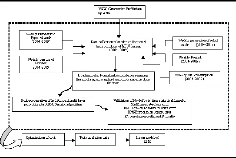
consumption for 4-ton truck is 30 Liter (L) and for 10- ton truck is 40 L in Langkawi, Malaysia. Framework of methodology for this research is shown on Figure 1.
Figure 1. Methodology framework for this study
The first approach in the RSM is to estimate the parameters of the model using the least-squares regression, and to determine the fitness of these parameters in an analysis of variance (ANOVA). The surface estimated is usually curved with a “hill” having peaks that appear at the exclusive estimated point of maximum response, and a “valley,” or a “saddle-surface” without any exclusive minimum or maximum response [58].
Numerous RSMs encouraged transforming the normal variables to coded variables x1, x2, x3,..., xk, which are usually defined to be dimensionless with signifying zero and the same standard deviation. In terms of the coded variables, the response function was presented by Mirhosseini et al. in 2007 as follows:
Y=f (x1, x2, x3,..., xk) (12)
125
The form of the first-order model is usually referred to as the most significant effect model, due to the fact that it incorporates only the major effects of the two variables x1 and x2. For instance, if a response variable y is measured, values are combinations of two factor
variables, x1 and x2. If there is an interaction between these variables, it can be easily added to the model as follow:
Y= β0+ β1x1+ β2x2+β 2x2 + β12x1x2 (14)
RESULTS AND DISCUSSION
The statistical analysis of waste materials in Langkawi Island in different months from 2004-2009 is presented in appendixes. Since the values of average and median are close, the amount of waste generation demonstrates a standard distribution in the seasons and weeks. Due to the high number of tourists during the peak season, the rate of WG increases rapidly. Various structures of feed forward ANN through three layers organization with several neurons quantity in the hidden layer were considered in this research to obtain the most excellent structure of ANN for calculating the waste generated.
With reference to Levenberg-Marquadte [60] as a training function and testing as a weekly average SW produced, we used the weekly fuel consumption,
weekly number and types of truck used for collection and transportation of the SW produced, weekly average number of personnel involved in the collection and transportation of SW, and weekly number of tourists were used in this analysis. And by applying MAE, MARE, RMSE, TS and R2, appropriate types of model were chosen in this study.
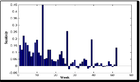
At first, the data were recorded in Excel, then transformed to MATLAB and normalization analysis was performed in equation (15). In the next step, sensitivity analysis was used to select the effective factors. In fact, sensitivity analysis attempts to find the existing relationship among the data.
Normalization Analysis = (x - MinX) / (MaxX - MinX) * 2 – 1 (15)
The sensitivity analysis in Figure 2 showed that the impact of peak seasons on the prediction of solid waste depends on generation of solid waste in the 26th, 39th and 52nd weeks prior to the peak seasons. To forecast the waste generated in the n-th week, waste generated in the previous 13 weeks (N-1 to N-13), the said weeks based on the findings of sensitivity analysis, average
number of trucks, number of tourists who visited the area, fuel consumed and the number of personnel in those weeks were used as input variablesto ANN with the structure of feed forward. The network training was performedaccording to the back propagation algorithm using the tangent hyperbolic function.
126
To obtain the best results, the genetic algorithm was used for network training and testing to optimize the number of hidden layers, to predict the amount of waste generated with 20 input layers (waste generation during the previous 13 weeks); amount of waste generated during the26th, 39th, and 52nd previous weeks, average number of personnel, tourists, types of truck and fuel consumption (based on the type of truck). In this step, the data were prepared to determine the effective elements considering the information obtained. The matrix in MATLAB included 20 columns and 260 rows. In the next step, validation assessment was made; quarterof theinput data was chosen as testing data set (random) and the remainder was used as training data set (i.e., 200 for training and 60 for testing, 52 in the sensitivity analysis). Finally, normalization of the data was performed. Afterward, the networks were arranged
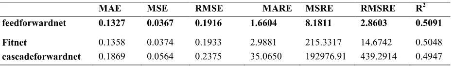
using feed forward net, fit net and cascade forward net to assess the network based on the three functions applied to the following errors; i.e., MAE (mean absolute error), MSE (mean squared error), RMSE (root mean squared error), MARE (mean absolute relative error), MSRE (mean squared relative error), RMSRE (root mean squared relative error) and R2. Based on the findings of the errors and R2, the feed forward net was selected for Langkawi Island. The results are shown in the Tables1,2,3 and 4. In Table 1 amounts of all errors are less in feed forward net and amount of R2 is bigger than the other function in training data. According to amount of errors in feed forward net for testing data and R2 it is better function for training. Amount of R2 in 'trainbr' function is higher than the others based on Table 2.
Table 1. Rate of errors on the training data for various functions of Feed forward net, fit net and cascade forward net (for selection of the best function of train)
MAE MSE RMSE MARE MSRE RMSRE R2
feedforwardnet 0.1327 0.0367 0.1916 1.6604 8.1811 2.8603 0.5091
Fitnet 0.1358 0.0374 0.1933 2.9881 215.3317 14.6742 0.5048
cascadeforwardnet 0.1869 0.0564 0.2375 35.0650 192976.91 439.2914 0.4947
Table 2. Rate of errors on the testing data for various functions of Feed forward net, fit net and cascade forward net (for selection of the best function of train)
MAE MSE RMSE MARE MSRE RMSRE R2
feedforwardnet 0.140 0.049 0.2227 2.2002 27.83 5.2757 0.599 Fitnet 0.1957 0.074 0.2715 3.9544 217.37 14.744 0.255
cascadeforwardnet 0.2467 0.145 0.3804 2.9933 65.866 8.1158 -0.067
Table 3. The Results of The errors for the training data in different functions due to select the best function
MAE MSE RMSE MARE MSRE RMSRE R2
'traingdx' 0.1462 0.0466 0.2159 5.3915 414.8412 20.3677 0.2390
'trainbr' 0.0316 0.0119 0.1090 0.2775 2.5797 1.6061 0.8824 'traincgb' 0.1018 0.0184 0.1356 5.7717 825.7565 28.736 0.7939
'traincgf' 0.1018 0.0184 0.1356 5.7717 825.7565 28.736 0.7939
'traincgp' 0.1098 0.0210 0.1451 3.0847 133.9714 11.5746 0.7575
'traingd' 0.1263 0.0322 0.1794 4.7661 642.8201 25.3539 0.5945
'traingda' 0.1358 0.0385 0.1961 15.6596 13324.0274 115.4298 0.4912
'traingdm' 0.1360 0.0468 0.2164 5.6301 306.8240 17.5164 0.2506
'trainbfg' 0.1125 0.0253 0.1590 2.0103 18.3127 4.2793 0.6991
'trainlm' 0.116 0.029 0.170 1.1677 3.6818 1.9188 0.6427
'trainoss' 0.1055 0.0182 0.1347 75.1768 1068795.0679 1033.8255 0.7951
'trainrp' 0.1100 0.0232 0.1524 6.2791 1522.7902 39.0229 0.7291
127
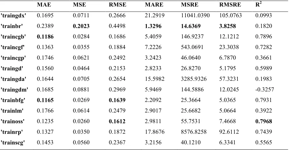
Table 4.The Results of The errors for the testing data in different functions due to select the best function
MAE MSE RMSE MARE MSRE RMSRE R2
'traingdx' 0.1695 0.0711 0.2666 21.2919 11041.0390 105.0763 0.0993
'trainbr' 0.2389 0.2023 0.4498 1.3296 14.6369 3.8258 0.1820
'traincgb' 0.1186 0.0284 0.1686 5.4059 146.9237 12.1212 0.7896
'traincgf' 0.1363 0.0355 0.1884 7.2226 543.0691 23.3038 0.7282
'traincgp' 0.1746 0.0621 0.2492 3.2423 46.0640 6.7870 0.3661
'traingd' 0.1560 0.0464 0.2153 2.8233 26.8270 5.1795 0.5989
'traingda' 0.1644 0.0705 0.2654 15.5982 3285.9326 57.3231 0.1983
'traingdm' 0.1685 0.0881 0.2969 5.9469 144.5886 12.0245 -0.3257
'trainbfg' 0.1165 0.0269 0.1639 2.2092 25.3664 5.0365 0.7931
'trainlm' 0.1766 0.0614 0.2479 2.9017 25.6682 5.0664 0.3922
'trainoss' 0.1235 0.0260 0.1612 2.9811 55.7531 7.4668 0.7968 'trainrp' 0.1327 0.0350 0.1872 17.8676 8576.8258 92.6112 0.7439
'trainscg' 0.1453 0.0560 0.2367 3.2156 40.1210 6.3341 0.5565
The next step was the selection of the best training function among the 13 functions in ANN.
Functions of 'trainbr' و 'trainbfg'و'trainoss' had the best answer; these functions were reassessed to obtain the
best answer with more accuracy. Table 5 showed errors during training and Table 6 illustrated errors for testing data.
Table 5. The errors on the training data for different functions due to select the most accurate function
MAE MSE RMSE MARE MSRE RMSRE R2
'trainbr' 0.0314 0.0191 0.1382 2.3294 841.8276 29.0143 0.8502 trainbfg 0.1077 0.0223 0.1492 10.8239 11825.3410 108.7444 0.7422
'trainoss' 0.1280 0.0299 0.1731 2.5434 112.9518 10.6279 0.6861
Table 6. The errors on the testing data for different functions due to select the most accurate function
MAE MSE RMSE MARE MSRE RMSRE R2
'trainbr' 0.2425 0.1278 0.3575 1.5873 6.3330 2.5165 0.2807
trainbfg 0.1376 0.0325 0.1802 7.0152 894.3073 29.9050 0.7469 'trainoss' 0.1517 0.0358 0.1891 3.4834 72.1797 8.4959 0.7526
Function of feed forward net with training function of trainbr were the best functions for modeling in Langkawi, which resulted from the optimization of number of hidden layers with genetic algorithm. Number of layers between 1- 4 tested and the number
128
number of (4) per chromosome. The selection mode was based on the random design between 0 and 1 (binary).The cost function (neuron numbers) per layer was equal to R2 minus one (1- R2). The primary selection was based on the direct random method from the population based on the lower cost (or higher R2). It was repeated 200 times and per time data was selected
based on the best result. Finally, 3 hidden layers were selected in this model, and the number of neurons were (31, 14, 24) and (9, 5, 11). If the number of neurons in the layers were more, the final answer would be deficient. The best answer of the ANN model is shown in the Figures 3, 4, 5 and 6.
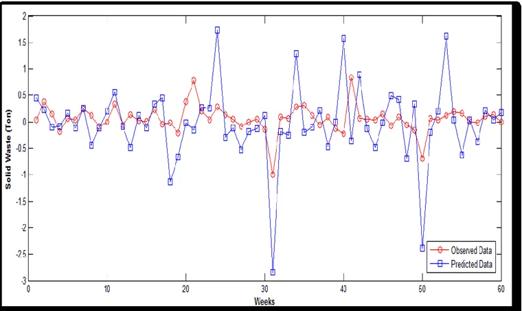
Figure 3. The observed amount of solid waste and the predicted output of ANN model with three neurons in the hidden layer for training data set in Langkawi Island (2004-2009).
129
Figure 5. The observed amount of solid waste and the predicted output of ANN Model with three neurons in the hidden layer for testing data set in Langkawi Island (2004-2009).
130
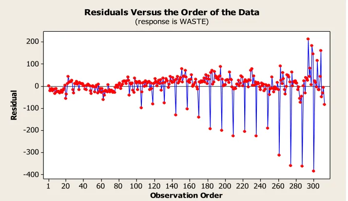
The final result of ANN model with optimization by genetic algorithm is shown in the Table 7. The validations of model and error histogram are shown in
the Figure 7; moreover Residuals versus based on observation order is in Figure 8. The validations of ANN for test and training are 94%.
Table 7. The calculated errors for ANNs with three neurons in the hidden Layers (based on the genetic algorithm) applied in training and testing data sets for Langkawi Island (2004-2009).
MAE MSE RMSE MARE MSRE RMSRE R2
Train 0.0847 0.0119 0.1093 5.1472 1226.79364 35.0256 0.87229 Test 0.1426 0.03587 0.1894 2.67084 31.6998 5.6302 0.711169
Figure 7. Validation of modeling with three neurons in the hidden layer,Validation of the ANN model in Langkawi.
Observation Order
R
es
id
ua
l
300 280 260 240 220 200 180 160 140 120 100 80 60 40 20 1 200
100
0
-100
-200
-300
-400
Residuals Versus the Order of the Data
(response is WASTE)
131
One of the most significant ANN characteristics is the number of neurons in the hidden layer. With an increase of the neurons in the hidden layer, the error was higher than the selected number of neurons in this study. However, the inadequate number of neurons applied to the network was not able to completely model the data.
In this study, the response surface analysis was performed, and the aim was to optimize the cost of collecting SW. Afterward, the relations between the independent variables and response variables were examined. The experimental data is presented in Table 8. The response surface analysis allowed an empirical relationship progress, where every response variable (Y1, Y2 and Y3) was measured as a function of X1 (number of personnel), X2 (number of trucks), and X3 (amount of fuel consumption), forecasted as the sum of
constant (β0), four first-order consequence (Linear Model terms in X1, X2, X3 and interaction effects
among them. The final outcome was investigated by using ANOVA to calculate the ‘‘goodness of fit’’. The conditions found to be statistically significant (p < 0.05) were considered in the model. As shown in the
following equation, the result and model for forecasting the response variables demonstrated the most important relationship and interaction between the variables. Table 9 and 10 presents the approximated regression coefficients of the polynomial response surface models with the corresponding R2 values and lack of fit tests. The significance of every element was specified by the F-ratio and p-value as presented in Tables 11 and 12. The values of "Prob > F" were less than 0.05 and the value indicating model terms was significant. Before using the model, it is important to ensure the normality of the data. Therefore, the NPar-test was used through IBM SPSS 19 and the result indicated that all the data met the normality requirement (Table 9 and 10). Table 11 explained model based on response cost. Table 13 demonstrated the characteristic of model, and Table 14 showed lower and upper limitation of identified variables based on the expert’s ideas for planning during collection and transportation of solid waste in Langkawi Island. Expert Design of research is showed in Figure 9; in addition validation of RSM model illustrated in Figure 10.
Table 8.Central composite design independent (Xi) and response variables (Yj), Langkawi Island (2010)
Treatment
Run Personnel Number (X1)
Fuel Liter (X2)
Lorry Number 10-ton (X3)
Lorry Number 4-ton (X4)
Solid Waste Ton (Y)
1 13708 22867.5 2700 1454 6932.3
2 14634 24409.5 2885 1547 7452.8
3 15694 26189.1 3083 1681 8032.3
4 14578 24457.8 2739 1811 7691.2
5 14500 24503.7 2556 2138 7780.4
6 14542 24489 2645 1981 7676.6
7 13850 23162.1 2673 1579 7558.9
8 13852 23237.3 2605 1716 7587.1
9 12832 21548.4 2392 1632 7172.9
10 12784 21371.3 2475 1442 7162.5
11 13446 22570.5 2515 1693 7669.9
12 13404 22462.4 2543 1616 7793.8
13 12346 20767.4 2268 1637 7185.8
14 12674 21399.2 2252 1833 7599.8
15 12836 21613.7 2337 1744 7871.2
16 12532 21060.5 2321 1624 7341.7
17 11754 19725.6 2203 1471 6862
18 11954 20046 2255 1467 7122
19 11718 19600.4 2258 1343 6586.6
20 12068 20258.7 2256 1522 6786.5
21 12972 20240.6 2523 1440 7300.7
22 13930 23196.6 2783 1399 7150.7
23 15000 24982.4 2993 1514 8399.1
132
Table 9. Correlation matrix of factors [Pearson's r] Table 10. Analysis of linear model in Langkawi
Table 11. Sequential model sum of squares based on the response cost
Source Sum of
Squares DF MeanSquare FValue Prob > F
Mean 1.170E+010 1 1.170E+010 3.973E+006 < 0.0001
Linear 9.554E+007 3 3.185E+007 6.93 0.0030 Suggested
2FI 88.23 3 29.41 0.86 0.4855 Suggested
Quadratic 11.20 3 3.73 19.89 0.0009 Aliased
Cubic 58.68 8 7.34
Residual 2.21 6 0.37
Total 1.179E+010 24 4.914E+008
Table 12. Analysis of variance table [Partial sum of squares] Source Sum of
Squares DF MeanSquare F Value Prob > F
Model 9.554E+007 6 1.592E+007 3.755E+006 < 0.0001
significant
A 1.896E+005 1 1.896E+005 44711.88 < 0.0001
B 3.279E+005 1 3.279E+005 77319.14 < 0.0001
C 22.04 1 22.04 5.20 0.0358
AB 39.26 1 39.26 9.26 0.0074
AC 34.80 1 34.80 8.21 0.0107
BC 23.74 1 23.74 5.60 0.0301
Residual 72.09 17 4.24
Cor Total
9.554E+007 23
Std. Dev 279.95
Mean 7439.27
C.V. 3.76
PRESS 2.246
R-Squared 0. 6315
A B A2 B2 AB
A 1.000
B 0.965 1.000
A2 0.734 0.657 1.000
133
Table 13. The model characteristics
Std. Dev 2.06 Mean 22076.46 C.V. 9.328 PRESS 10919.74 Pred R-Square 0.9999 Adeq Prediction 6218.082
Table 14. Constraints of planing for collection and transportation of solid waste in langkawi Island, lower and upper limit are identified based on the experts ideas and suggestions
Name Goal Lower
Limit Upper Limit Lower Weight Upper Weight Personnel is in a
range 10000 16000 1 1
Fuel is in a range
19725 25000 1 1
Total
Truck is in a range 1300 5000 1 1
Solid Waste
is in a range
7986.6 8399.1 1 1
Cost minimize 19193.7 26110.4 1 1
Figure 9. Design expert plot cost in Langkawi
134
Figure10. Validation of RSM model for SW response by excel in Langkawi Island
Final Equation in Terms of Coded Factors:
(Solid Waste) = 3163.084-0.053088 * Personnel +1.49818* Total truck - 0.056234*fuel (16)
This study used a linear response surface. The full quadratic response surface is shown to be the most efficient approximation to fit the finite element model.
Based on the existing facilities and other parameters as well as the linear model, the best use of machinery and
labor, and the minimum cost in the collection and transportation of waste are presented in Table 14, and Figure 9. Table 15 shows scenario according to interview with the experts.
Table 15. Number optimization-set goals for each response
No. Personnel Fuel Total
Truck Waste Solid Cost Desirability
1 10488.57 17358.13 4278.20 8039.68 14873.6 1.000 Selected
2 11677 17566.6 4321.32 8029.46 17540.6 1.000
3 10470.8 22727.76 4572.16 8281.53 14156.2 1.000
4 12177.42 18636.55 4591.83 8348 18079.5 0.999
The 3D response surfaces model in linear form showed the best significant relationship (p < 0.05). The interaction effects of the independent variables were plotted based on the cost optimization related to the solid waste collection and transportation. The plots are
135
Table 16. Prediction and estimation of solid waste management cost in Langkawi Island
Factors Autumn
2009 Spring 2011 Unit cost RM Sum cost Aut 2009 Sum cost Spr 2011 Solid waste 7825.7 (ton) 8039.68
(ton)
- - -
Personnel 15666
(person) 10488.57 (person) 3.75 58747.5 39332.14
Total fuel consumption
171690 (liter)
157353.1 (liter)
1.9 326211 298970.8
Total Truck
(maintenance,repair and rent)
4668
(number) (number) 4278.20 60,40 250020 229142.2
Total cost - 634978.5 567445.1
Notes : 15666 trips made by individual worker within three months
The total cost of collection and transportation of solid waste in Langkawi Island in 2009reached RM 67533.4; therefore,
634978.5 - 567445.1= 67533.4
67533.4*100/634978.5= 10.63554 %
This means that in spite of the increase in population and generation of solid waste in 2011, the use ofRSM showed 10.63 percent reduction in cost in Langkawi Island.
The first step was to set up a design and then arrange the data collected from 2004 to 2009 in form of per three months, and the second step was to prepare the model based on the experimental settings. The third step was to apply ANOVA to fit the model and calculate the fitting model and error. The last step was the verification and validation of the model by statistical analysis. From the findings, the use of the linear function of the response surface model appeared to be effective in the Island.
In the autumn season of 2009, the amount of solid waste generated in Langkawi Island was 7825.7 tons and it took 15666 trips per person into the landfill, 171690 liters of fuel and 4668 total trips made by the trucks to transport this amount of waste to the landfill. In spring 2011, the amount of solid waste generated increased to 8039.68 tons, while based on the linear RSM model, number of times that personnel entered the landfill to work on solid waste decreased to 10488.57 times, fuel consumption for carrying this amount of waste decreased to 157353.1 liters and the number of
trips made by the trucks decreased to 4278.20 times. The analysis was undertaken using the primary data collected through interview with experts in the Municipality regarding daily wages per person (i.e., salary of person for collection and transportation of MSW) which is equivalent to 10 dollars; per fuel liter is equivalent to 63 cents; Fuel consumption for 4-ton truck is 30 L and for 10-ton truck is 40 L in Langkawi, Malaysia.
Also, the cost of maintenance related to repair and rent of trucks was computed. In 2011, a total of 4278.20 trips were made to the landfill, i.e., 1378 times by the 4-ton trucks and 2900 times by the 10-4-ton trucks. The total cost incurred during the autumn season in 2009 was RM 634978.5, which reduced to RM 567445.1 in spring in 2011.
CONCLUSION
This research has combined ANN and RSM withmore input variables to predict or forecast solid waste generation andoptimize the cost of waste collection and transportation in Langkawi Island. The objective in combing the two models was to provide knowledge about the amount or quantity of solid waste generated over time and how to optimize the related cost, which the authors believe will assist the authorities who are in-charge of solid waste management to design appropriate and cost effective measures to collect and transport solid waste in general and in Langkawi in particular.
136
facilitate achieving the objectives of solid waste management, particularly in Langkawi, Malaysia. The use of ANN model showed increasing amount of solid waste generation in relation to the increasing number of tourists. Therefore, the activities of the Environment
Idaman Sdn Bhd, a local waste management company which is involved in solid waste management in Kedah, should be fully supported financially and technically. This is because the cost involved in the programs to minimize solid waste generation will be lower than the solid waste collection, transportation and treatment at the landfills. For that reason, more private companies should be enticed by the Malaysia Government into the business of solid waste management, particularly in activities focusing on minimizing solid waste generation.
REFERENCES
1. Sara Ojeda Benítez, Gabriela Lozano-Olvera, Raúl Adalberto Morelos, Carolina Armijo de Vega. (2008). Mathematical modeling to predict residential solid waste generation. Waste Management 28, S7–S13.
2. Zhu Minghua, Fan Xiumin, Alberto Rovetta, He Qichang, Federico Vicentini, Liu Bingkai, Alessandro Giusti, Liu Yi. (2009). Country Report, Municipal solid waste management in Pudong New Area, China. Waste Management 29, 1227–1233.
3. Sujauddin, M., Huda, M.S., Rafiqul Hoque, A.T.M.. (2008). Household solid waste characteristics and management in Chittagong, Bangladesh. Journal of Waste Management 28, 1688–1695.
4. Burntley, S.J. (2007). A review of municipal solid waste composition in the United Kingdom. Journal of Waste Management 27 (10), 1274– 1285.
5. Lilliana Abarca Guerrero, Ger Maas, William Hogland. (2013). Review Solid waste management challenges for cities in developing countries. Waste Management, Volume 33 (1) 220–232.
6. Daskalopoulos, E., Badr, O., Probert, S.D. (1997). Economic and environmental evaluations of waste treatment and disposal technologies for municipal solid waste. Appl Energy 58(4): 209– 255.
7. Noori, R., Abdoli , M. A., Ameri, A., Jalili-Ghazizade, M. (2009). “Prediction of Municipal Solid Waste Generation with Combination of Support Vector Machine and Principal Component Analysis: A Case Study of Mashhad”. Environmental Progress & Sustainable Energy 28 (2): 249-258.
8. Noori, R., Abdoli, M.A., Jalili Ghazizade, M. Samieifard, R. (2009). Comparison of Neural Network and Principal Component-Regression Analysis to Predict the Solid Waste Generation inTehran. Iranian J Publ Health 38 (1):74-84.
9. Tavares, G. Zsigraiova, Z. Semiao, V., Carvalho, M.G. (2009). Optimisation of MSW collection routes for minimum fuel consumption using 3D GIS modeling, Waste Management 29(3):1176– 1185.
10. UNDP (United Nations Development Programme). (1997). “Survey of Mayors: Major Urban Problems.” UNDP, Washington, DC.
11. Jalili Ghazi Zade, M. Noori, R. Winter (2008). Prediction of Municipal Solid Waste Generation by Use of Artificial Neural Network: A Case Study of Mashhad. Int. J. Environ. Res. 2(1):13-22. ISSN: 1735-6865.
12. Chang, Ni Bin. (1991). “Environmental System Analysis of Solid Waste management.” PhD Dissertation, Cornell University.
13. Sara Ojeda Benítez, Gabriela Lozano-Olvera, Raúl Adalberto Morelos, Carolina Armijo de Vega. (2008). Mathematical modeling to predict residential solid waste generation. Waste Management 28, S7–S13.
14. Jalili Ghazi Zade, M. Noori, R. Winter (2008). Prediction of Municipal Solid Waste Generation by Use of Artificial Neural Network: A Case Study of Mashhad. Int. J. Environ. Res. 2(1):13-22. ISSN: 1735-6865.
15. Rimaityte I, Ruzgas T, Denafas G, Racys V, Martuzevicius D. (2012). Application and evaluation of forecasting methodsfor municipal solid waste generation in an Eastern-European city. Waste Management Res, jan 30 (1): 89-98.
137
Chile. Proc. Waste and Recycle. Fremantle, Australia ,pp.1-11.
17. Baluja, S. (1994). Population-Based Incremental Learning: A Method for Integrating Genetic Search Based Function Optimization and Competitive Learning. Carnegie Mellon: CMU-CS-94-163.
18. Hamseveni, D.R., Prapulla, S.G., Divakar, S. (2001). Response surface methodological approach for the synthesis of isobutyl isobutyrate. Proc Biochem 36:1103–9.
19. Pelikan, M., Muhlenbein, H. (1999). The Bivariate Marginal Distribution Algorithm, Advances in Soft Computing-Engineering Design and Manufacturing. Springer-Verlag 521-535.
20. Anderson, L.E. (1968). A mathematical model for the optimization of a waste management system University of California at Berkeley, Sanitary Engineering Research Laboratory, SERL USA, No. 68-1.
21. Chang, N. B., Chen ,Y. L., Wang, S. F. (1997). A fuzzy interval multiobjective mixed integer programming approach for the optimal planning of solid waste management systems. Fuzzy Sets and Systems 89 (1): 35-60.
22. Huang, G. H., Chi, G. F., & Li, Y. P. (2005). Long-term planning of an integrated solid waste management system under uncertainty-I. Model development Environmental Engineering Science 22(6): 823-834.
23. Ogwueleka, TC. (2009). Municipal solid waste characteristics and management in Nigeria. Iranian Journal of Environmental Health Science and Engineering 6(3): 173-180.
24. Marković, Danijel., Janošević, Dragoslav., Jovanović, Miomir., Nikolić, Vesna. (2010). Application Method For Optimization In Solid Waste Management System In The City Of NIŠ, Series: Mechanical Engineering 8(1): 63 – 76.
25. Dogan, K., Su¨leyman, S. (2003). Report: cost and financing of municipal solid waste collection service in Istanbul. Waste Management and Research 21: 480–485.
26. Tung, D.V., Pinnoi, A., (2000). Vehicle routing-scheduling for waste collection in Hanoi.
European Journal of Operational Research 125(3): 449–468.
27. Johansson, Ola M. (2006). The effect of dynamic scheduling and routing in a solid waste management system, Waste Management 26(8): 875–885.
28. Tariq Bin Yousuf & Mostafizur Rahman. (2007). Monitoring quantity and characteristics of municipal solid waste in Dhaka City, Environ Monit Assess 135:3–11, DOI 10.1007/s10661-007-9710-6. (On line, 28 Aug 2012).
29. Erin, R. G. (2005). Factors effecting the optimization of lipase-catalyzed palm based esters synthesis. (unpublished) PhD Thesis. Universiti Putra Malaysia.
30. Montgomery D. C. (2001). Design and analysis of experiments. New York: John Wiley and Sons, 427-450.
31. Montgomery, J.M., Pavlidis, P., Madison, D.V. (2001). Pair recordings reveal all-silent synaptic connections and the postsynaptic expression of long-term potentiation. Neuron re29 (3): 691– 701.
32. Marković, Danijel., Janošević, Dragoslav., Jovanović, Miomir., Nikolić, Vesna. (2010). Application Method For Optimization In Solid Waste Management System In The City Of NIŠ, Series: Mechanical Engineering 8(1): 63 – 76.
33. Ashtashil Vrushketu Bhambulkar. (2011). Municipal solid waste collection routes optimized with arc gis network analyst. International Journal Of Advanced Engineering Sciences And Technologies Vol No. 11, Issue No. 1, 202 – 207.
34. Katkar, Mr.Amar A. (2012). Improvement of Solid Waste Collection by Using Optimization Technique. International Journal of Multidisciplinary Research 2(4), ISSN 2231 5780.
35. Chen, M.C.; A. Ruijs, J. Wesseler. (2005). “Solid Waste Management on Small Islands: The Case of Green Island, Taiwan”, Resources, Conservation and Recycling, vol. 45, no 1, p. 31-47.
138
Municipal Solid Waste Management Planning in Small Island Developing States in the Pacific Region.
37. Mohd Shafeea Leman, Ibrahim Komoo, Kamal Roslan Mohamed, Che Aziz Ali, Tanot Unjah, Kasim Othman& Mohd Hizamri Mohd Yasin. (2008).Geology and geoheritage conservation within langkawi geopark, Malaysia. Articles and Publications.(online)http://www.globalgeopark.o rg/Articles/6337.htm. (2 March 2013).
38. Nadi, B., Mahmud, A. R., Shariff, A. R., Ahmad, N. (2010). Prediction of Solid Waste Base on Artificial Neural Network. Proceeding of the WEC CGAG-Conference on Geomatics and Geographical Information Science, Kuching, Sarawak, Malaysia.
39. Jalili Ghazi Zade, M. Noori, R. Winter (2008). Prediction of Municipal Solid Waste Generation by Use of Artificial Neural Network: A Case Study of Mashhad. Int. J. Environ. Res. 2(1):13-22. ISSN: 1735-6865.
40. Chung, Shan Shan. (2010). Projecting municipal solid waste: The case of Hong Kong SAR, Resources, Conservation and Recycling 54(11) 759–768.
41. Maier, H.R., Dandy, G.C. & Burch, M.D. (1998). Use of artificial neural networks for modelling cyanobacteria anabaena Spp. In the River Murray, South Australia. Ecological Modelling 105(23): 257-272.
42. Palani, S., Liong, S.Y., Thalich, P. (2008). An ANN application for water quality forecasting. Marine Pollut. Bull 56:1586-1597.
43. Ali, Najah. (2012). Prediction of water quality parameters utilizing several artificial intelligence techniques. (unpublished) Ph.D thesis, University Kebangsaan Malaysia.
44. Velmurugan, L.,. P. Thangaraj. (2012). A hidden genetic layer based neural network for mobility prediction.American Journal of Applied Sciences 9 (4): 526-530.
45. Osman Ahmed, Mohd Nordin, Suziah Sulaiman, Wan Fatimah. (2009). Study of genetic algorithm to fully-automate the design and training of artificial neural network. International Journal of Computer Science and Network Security 9 (1) (online)
http://paper.ijcsns.org/07_book/200901/2009013 1.pdf (28 January 2013).
46. Twomey, Janet. M. & Smith, Alice E. (1996). Validation and Verification. Kartam ,NAbil, Flood, Ian., Garret, James H Jr, (eds.) artificial neural networks for civil engineers: fundamentals and applicatons. New York: ASCE, 44-46.
47. Yang, J., Greenwood, D.J., Rowell, D.L., Wadsworth, G.A., Burns, I.G. (2000). Statistical methods for evaluating a crop nitrogen simulation model. N_ABLE, Agricultural Systems 64(1) 37-53.
48. Yorucu, Vedat. (2003). The Analysis of Forecasting Performance by Using Time Series Data for Two Mediterranean Islands, Review of Social. Economic & Business Studies 2175-196.
49. Department Of Treasury. (2008). Forecasting Accuracy of the Act Budget Estimates, Forecasting Accuracy Comparison, May. (online)
(http://www.treasury.act.gov.au/documents/Fore
casting%20Accuracy%20-%20ACT%20Budget.pdf) (20 December 2011).
50. Kumar, Jha Dilip., Sabesan, M., Das, Anup., Vinithkumar, N.V., Kirubagaran, R. (2011). Evaluation of Interpolation Technique for Air Quality Parameters in Port Blair. India. Universal Journal of Environmental Research and Technology 1 (3): 301-310.
51. CarmeliaM. Dragomir,WimKlaassen, Mirela Voiculescu, Lucian P. Georgescu, Sander van der Laan. (2012). Estimating Annual CO2 Flux for Lutjewad Station Using Three Different Gap-Filling Techniques, The ScientificWorld Journal,vol.2012. (online) http:// www.tswj.com /2012/842893/ ( 31 August 2012).
52. Haykin, S. (1994). Neural networks: A comprehensive foundation (2nd ed.). New York: Macmillan.
53. Simon Haykin. (2009). Neural network and learning machines-3rd ed. (Pearson Prentice Hall,).
139
55. Tanyildizi, M. Saban; Ozer, Dursun, Elibol, Murat. (2005). Optimization of α-amylase production by Bacillus sp. using response surface methodology. Process Biochemistry 40(7): 2291-2296.
56. Hounsa, C.G., Aubry, J.M., Dubourguier, H.C. (1996). Application of factorial and Doehlert design for optimization of pectate lyase production by a recombinant Escherichia coli. Appl Microbiol Biotechnol 45:764–70.
57. Hamseveni, D.R., Prapulla, S.G., Divakar, S. (2001). Response surface methodological approach for the synthesis of isobutyl isobutyrate. Proc Biochem 36:1103–9.
58. Erin, R. G. (2005). Factors effecting the optimization of lipase-catalyzed palm based esters synthesis. (unpublished) PhD Thesis. Universiti Putra Malaysia.
59. Keshani, S., Luqman Chuah, A., Nourouzi, M. M., Russly A.R. & Jamilah, B. (2010). Optimization of concentration process on pomelo fruit juice using response surface methodology (RSM). International Food Research Journal 17(3): 733-742.
60. Yu, H., and B. M. Wilamowski, (2011). “Neural Network Training with Second Order Algorithms,” Human-Computer Systems Interaction. Background and Applications 2 Series: Advances in Intelligent and Soft Computing (99 Part II) Springer-Verlag, pp. 463-476.
61. Agatonovic-Kustrin, S., Zecevic, M., Zivanovic, L.,Tucker,I.G.,(1998). Application of neural networks for response surface modeling in HPLC optimization. Analytica Chimica Acta 364, 256–273.
62. Apaydin O., Gonullu M.T. (2008). Emission control with route optimization in solid waste collection process: A case study, Sadhana, 33(2): 71-82.
63. Apaydin, O., Gonullu, M.T. (2011). Route Time Estimation Of Solid Waste Collection Vehicles Based On Population Density, Global NEST Journal 13(2): 162-169.
64. Apaydin O., Gonullu M.T. (2007) Route Optimization for Solid Waste Collection: Trabzon (Turkey) Case Study, Global NEST J., 9, 6-11.
65. Baumes, L., Farrusseng, D., Lengliz, M., Mirodatos, C. (2004). Using artificial neural networks to boost high-throughput discovery in heterogeneous catalysis. QSAR & Combinatorial Science 29, 767–778.
66. Box, G. E. P., Draper, N. R. (1987). Empirical Model Building and Responses Surfaces. New York: Wiley.
67. Castillo ED. (2007). Process optimization a statistical approach, vol. 97. New York, USA, New York: Springer; p. 97.
68. Daskalopoulos, E., Badr, O., Probert, S.D.. (1998). Municipal solid waste: a prediction methodology for the generation rate and composition in the European Union countries and the United States of America. Resources, Conservation and Recycling 24, 155–166.
69. F. Karimi, S. Rafiee, A. Taheri-Garavand, M. Karimi. (2012). Optimization of an air drying process for Artemisia absinthium leaves using response surface and artificial neural network models. Journal of the Taiwan Institute of Chemical Engineers. 43, 29–39.
70. Goldberg D.E. (1988). Genetic algorithms in search, optimization and machine learning, Addison- Wesley.
71. Guoyi Chi, Shuangquan Hu, Yanhui Yang, Tao Chen. (2012). Response surface methodology with prediction uncertainty: A multi-objective optimization approach. Chemical engineering research and design. 90, 1235–1244.
72. Harik, G. (1997). Learning gene linkage to efficiently solve problems of bounded difficulty using genetic algorithms. Ph.D. thesis. University of Michigan.
73. Navarro-Esbrı , J. E. Diamadopoulos, D. Ginestar. (2002). Time series analysis and forecasting techniques for municipal solid waste management. Resources, Conservation and Recycling 35, 201 – 214.
74. Matsuto T, Tanaka N. (1993). Data analysis of daily collection tonnage of residential solid waste in Japan. Waste Manage Resourc; 11:333–43.
140
stability, viscosity, fluid behavior, ζ-potential and electrophoretic mobility of orange beverage emulsion using response surface methodology. J. Agr. Food Chem. 55:7659-7666.
76. Mohammad Hindi Bataineh. (2012). Artificial Neural Network for Studying Human Performance. The University of Iowa.
77. Mrayyan, B., & Hamdi, M.R. (2006). Management approach to integrated solid waste in industrialized zones in Jordan: a case of Zarqa City. Waste Management 26(2) 195–205.
78. M¨uhlenbein, H. & Paaß, G. (1996). From recombination of genes to the estimation of distributions I. binary parameters. Lecture Notes in Computer Science 1141: pages 178–187, Springer Verlag, Berlin.
79. Muhlenbein, H. (1998). The Equation for Response to Selection and its Use for Prediction. Evolutionary Computation 5(3): 303-346.
80. Muller, M., & Hoffman, L. (2001). Community partnerships in integrated sustainable waste management, WASTE, CW Gouda, The Netherlands, website: www.waste.nl.
81 Myers, R. H., Montgomery DC. (1995). Response Surface Methodology. New York: John Wiley & Sons.
82. Noori, R., Khakpour, A., Omidvar, B., Farokhnia, A. (2010). Comparison of ANN and principal component analysis-multivariate linear regression models for predicting the river flow based on developed discrepancy ratio statistic. Expert Systems with Applications 37 (8) 5856– 5862.
83. Rahardyan, B., Matsuto, T., Kakuta, Y., Tanaka, N. (2004). Residents’s concerns and attitudes towards solid waste management facilities. Waste Management 24(5): 437–451.
84. The International Bank for Reconstruction and Development/World Bank. (1999). What A Waste: Solid Waste Management in Asia.


![Table 9. Correlation matrix of factors [Pearson's r]](https://thumb-us.123doks.com/thumbv2/123dok_us/8456355.1706877/15.612.69.414.441.619/table-correlation-matrix-of-factors-pearson-s-r.webp)

