Analysis of Ion-Temperature-Gradient Instabilities Using a
Gyro-Fluid Model in Cylindrical Plasmas
∗
)
Genryu HATTORI, Naohiro KASUYA
1)and Masatoshi YAGI
2)Interdisciplinary Graduate School of Engineering Sciences, Kyushu University, 6-1 Kasuga-Koen, Kasuga, Fukuoka 816-8580, Japan
1)Research Institute for Applied Mechanics, Kyushu University, 6-1 Kasuga-Koen, Kasuga, Fukuoka 816-8580, Japan
2)Japan Atomic Energy Agency, 2-166 Omotedate, Obuchi, Rokkasho-mura, Aomori 039-3212, Japan
(Received 25 November 2014/Accepted 2 March 2015)
The excitation condition for ion-temperature-gradient (ITG) instabilities in linear devices is investigated us-ing a gyro-fluid equation. The finite-Larmor-radius effect is included in the model, which helps to stabilize ITG instabilities. The critical values ofη, which is the ratio of the lengths of the density gradient to the temperature gradient, are obtained. Although the modenumbers of the most unstable modes are different with different dis-charge gases, their critical values have almost the sameηlevel close to 1.0. The results are compared with those from the Hamaguchi–Horton model numerically and analytically.
c
2015 The Japan Society of Plasma Science and Nuclear Fusion Research
Keywords: ion-temperature-gradient instability, finite-Larmor-radius effect, gyro-fluid equation, linear device DOI: 10.1585/pfr.10.3401060
1. Introduction
Anomalous transport is one of the important issues in magnetic confined plasmas. Competition of several kinds of instabilities determines the formed turbulent struc-ture, and the level of turbulent transport [1]. One of the causes for turbulent transport is an ion-temperature-gradient (ITG) driven microscopic instability (ηi mode)
[2]. It has been predicted to be unstable when ηi (=
L−1
T /L−n1) exceeds some threshold, where the inverse of the
density gradient length and the ion temperature gradient length areL−1
n (=−d(lnn0)/dr) andLT−1 (=−d(lnT0)/dr),
respectively. Analyses of the ITG instability using fluid models and models including kinetic effects have been per-formed [3–5].
In experiments with high-temperature plasmas, it is difficult to identify the ITG instability because of the lim-ited diagnostics available. Conversely, in laboratory plas-mas using linear machines, detailed measurements of fluc-tuations can be conducted to identify the ITG instability [6]. In PANTA device [7], an ion sensitive probe and a laser induced fluorescence are used to measure temperature fluctuations. Furthermore, by employing phase tracking, nonlinear waveforms of fluctuations can be identified [8] to evaluate the heat flux. Numerical simulations for the linear growth rate of the ITG instability have also been in-vestigated using the fluid model in PANTA, which shows that the mode withk⊥ρs∼O(1) is unstable even with a low ion temperature [9]. Here,k⊥andρsare the wavenumber
in the perpendicular direction and the effective Larmor
ra-author’s e-mail: [email protected]
∗)This article is based on the presentation at the 24th International Toki Conference (ITC24).
dius, respectively. Therefore, it is necessary to include the finite-Larmor-radius (FLR) effect so as to perform a more quantitative analysis.
The target of this research is to clarify the excitation condition of ITG instabilities in the linear device PANTA. The ion Larmor radius is comparable to the plasma radius in linear devices, so we are developing a simulation code using a gyro-fluid model to include the FLR effect. By linearizing the model, the excitation condition of the ITG instability is evaluated. The local model is used for the first step. This paper is organized as follows. In the next sec-tion, the set of gyro-fluid equations is described. In Sec. 3, the excitation condition of the ITG instability is evaluated by local linear analyses. Comparison between the gyro-fluid and gyro-fluid model is performed in Sec. 4. The results are summarized in Sec. 5.
2. Model Equations
A set of gyro-fluid equations is derived by taking the moments of the following nonlinear electrostatic gyro-kinetic equation in the velocity spaces [10]:
∂F
∂t +∇ ·
Fv//bˆ+J0vE− ∂
∂v// e
mFbˆ· ∇J0Φ
=0, (1)
whereF is the distribution function,v//is the parallel ve-locity, ˆb is the unit vector in the direction parallel to the magnetic field,vEis theE×Bdrift velocity,Φis the
elec-trostatic potential, and J0 is a linear operator to perform gyro-averaging. The target plasma has a cylindrical con-figuration with a homogeneous magnetic field parallel to the axial direction, so the magnetic curvature terms can
c
2015 The Japan Society of Plasma
be eliminated. Applying gyro-kinetic ordering, the linear forms of the equations are as follows:
dn
dt +∇//n//
1+ηi⊥ 2 ∇ˆ
2
⊥ 1
Ln ∂Ψ
r∂θ =0, (2) du//
dt +∇//(nτ//+T//+Ψ)=0, (3) 1
τ
dT
dt +∇//(2u+q)+ηi// 1 Ln
∂Ψ
r∂θ
=−2vii
3τ(T//−T⊥), (4)
1
τ⊥ dT⊥
dt +∇//q⊥
1 2∇ˆ
2
⊥+ηi⊥
1+∇ˆˆ2 1 Ln
∂Ψ
r∂θ
= vii
3τ(T//−T⊥), (5)
where n is the ion density, u is the ion velocity, Ψ is the gyro-averaged potential in which Ψ ≡ Γ10/2Φ and
τ=T/Te,T is the ion temperature,Teis the electron
tem-perature,q is the heat flux, νii is the collision frequency
between the ions, andρsis the effective Lamor radius
eval-uated from the electron temperature. The subscripts//and
⊥represent the quantities parallel and perpendicular to the direction of the magnetic field, respectively. Pade andJ0 2
=Γ0approximations are applied, where Γ1/2
0 =
1
1+bτ⊥
2
, (6)
bτ⊥=−∇2⊥=τ⊥k2r+k2θ. (7) Collisions are dominant in this system, and higher order moments of Eq. (1) give simplified forms of the heat flux as follows [11]:
q//=− 3
viiτ⊥∇//T//, (8) q⊥=− 1
viiτ⊥∇//T⊥. (9) The quasi-neutrality relation is given to be
Γ0
n+ 1
τ⊥
∇2
⊥ 2 T⊥
−(1−Γ0)τΨ
⊥ =Ψ. (10) The FLR effect gives the difference between the local density and potential. Our gyro-fluid model consists of Eqs. (2 - 5) and (10). The FLR effect is included inΨ, ˆ∇2
⊥ and ˆˆ∇2terms, where
ˆ
∇2
⊥ 2 Ψ≡ −
bτ⊥
2
1+bτ⊥
2
Ψ, (11)
ˆˆ
∇2Ψ≡
bτ⊥
2
bτ ⊥
2 −1
1+bτ⊥
2
2 Ψ. (12)
The following normalizations are used:
r/ρs→r, (13)
Ωcit→t, (14)
n1
n0,
u// cs,
T//1
Te ,
T⊥1
Te ,
q//1
n0T//0cs,
q⊥1
n0T⊥0cs,
eΨ Te
→(n,u//,T//,T⊥,q//,q⊥, Ψ), (15)
where Ωci = eB/mi is the ion cyclotron frequency, cs = Ωciρs is the ion sound velocity, and the subscripts 0 and 1
denote the equilibrium and fluctuating component, respec-tively.
3. Linear Growthrate Analysis
Local linear analyses are conducted to evaluate the ex-citation condition of the ITG instability. To linearize the set of equations, the differential operators d/dt,∇//and∇⊥are replaced byλ,ikz, andik⊥, where the real and imaginary
part ofλare the growthrate and frequency,kzandk⊥are the
wavenumber in the parallel and perpendicular direction, re-spectively. This is a local model, so the results are basically the same as those with a slab geometry. The size of the plasma is reflected in the values of the mode numbers. The axial mode number is assumed to be 1, which giveskz =
2π/l, wherelis the device length. The radial and azimuthal wavenumbers are assumed to be the same (kr =kθ), which
givesk2
⊥ =2k2θ =2(m/r)2, wheremis the poloidal mode
number. The radial wavelength is approximately 2afor the fundamental ITG modes [9], so this assumption is used. This is a simplification for qualitative understanding, and the global mode analysis including the radial structure will be considered in future work. For linear analysis, experi-mental parameters in PANTA are used:l=4.0 m, plasma radiusa=7.0 cm, densityn=1.0×10¹⁹m−3,L
n=7.0 cm, νii=350 s−1, magnetic fieldB=0.1 T, which givesΩci/2π
=1.5 MHz. TemperaturesTe=3 eV andTi=0.3 eV give ρs=1.1 cm andρi=3.5 mm. With these parameters,ρi/Ln
=0.051.0,kzρi=5.5×10−31.0 andk⊥ρi=0.02
1.0, so gyro-kinetic ordering is satisfied. The other param-eters for the analysis areτandηi, which correspond to the
ratios between ions and electrons. Here, linear growthrates atr=a/2 are calculated.
First, the excitation conditions with different dis-charge gases are analyzed. In Fig. 1, the ion mass depen-dences of criticalηcof the modes withm=1 - 5 are shown.
The cases of helium, neon, and argon are plotted. The min-imum values ofηcare close to 1 even though the ion mass
numbers are different. This result suggests that there is no preferential gas for the ITG excitation. However, mode-numbers of most unstable modes depend on the discharge gasses (He: m=5, Ne and Ar: m=2), so the azimuthal mode structure can be different for fluctuations.
Fig. 1 Ion mass dependences of criticalηc, whenτ=1. Those
of modes withm=1 - 5 are plotted.
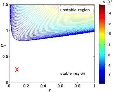
Fig. 2 Contour plot of the growth rate in theτandηspace. The boundary for unstable ITG mode is shown. The cross represents one set of experimental conditions in PANTA.
changes depending on the magnitude ofτ. The minimum
ηc=0.81 is given withτ=0.15, andηcincreases asτ
in-creases (e.g.,ηc=0.98, whenτ=1.0). Whenτis low (τ 0.15),ηcis large and the ITG mode is rarely unstable.
The cross in Fig. 2 indicates one set of experimental con-ditions in PANTA (τ=0.1,η=0.2 with argon discharge). It suggests that a larger temperature gradient is needed to observe the excitation of the ITG mode in PANTA.
Characteristic dependencies of the threshold value are evaluated next. Our model includes the FLR effect, which depends on the magnitude of variableb, so the FLR effect is investigated by varyingb. In Fig. 3, a contour plot of the growthrate in thebandηspace is shown. The critical
ηc increases withb, so the FLR effect stabilizes the ITG
mode. Notes that the PANTA parameter gives b = 0.8. In addition, our model contains a thermal anisotropy as in Eqs. (4) and (5), so the anisotropic case withη// η⊥ can be analyzed. In Fig. 4, a contour plot of the growthrate in theη//andη⊥space is shown. Fitting the critical boundary to the linear equationαη⊥+η//=Const givesα=2.1±0.1. The degree of freedom is 2 in the perpendicular direction,
Fig. 3 Contour plot of the growth rate in thebandηspace. This is the case withτ=1.0 of argon plasma.
Fig. 4 Contour plot of the growthrate in theη//andη⊥ space. This is the case withτ=1.0 of argon plasma.
which corresponds to the obtainedαvalue.
4. Comparison of the Gyro-Fluid and
Fluid Model
We have used the gyro-fluid model to evaluate the ITG excitation condition in PANTA. Conversely, the ITG anal-yses have been conducted using the Hamaguchi–Horton (H–H) model, which consists of fluid equations [12, 13]. The results from the H–H model show that the critical tem-perature gradient is smaller than that with the gyro-fluid model. Comparison between these two models is shown in this section.
The H–H model solves three fields with the ion conti-nuity equation, momentum conservation equation, and en-ergy conservation equation:
∂ ∂t
1− ∇2⊥φ+∇//u//+ 1 Ln
∂φ
r∂θ+τ 1 LP
∂
r∂θ
∇2
⊥φ
Fig. 5 Contour plot of the growthrate in theτandηspace with the H–H model. This is the case of argon plasma.
∂u//
∂t +∇//(φ+P)=0, (17)
∂P
∂t +γτ∇//u//+τ 1 LP
∂φ
r∂θ =0, (18) wherePis the ion pressure. For comparison, a reduced set of the gyro-fluid model equations is obtained with isotropic temperatureT//=T⊥ =T as
∂ ∂t
1−
1+1
τ∇2⊥ φ+∇//u//+ 1 Ln
∂φ
r∂θ
+1
2 1 LT
∂
r∂θ(∇
2
⊥φ)=0, (19)
∂u//
∂t +
1+τ+bτ
1+1
τ ∇//φ+
1+bτ 2
∇//T
=0, (20)
∂T
∂t + 2
3τ∇//u//+τ 1 LT
∂φ
r∂θ =0. (21) Here, the heat-flux terms and the FLR terms in Eqs. (2 - 5) are neglected, and the FLR term with variableb is only retained in the quasi-neutrality relation given in Eq. (10). Equation (21) is obtained by adding Eqs. (4) and (5). The basic frameworks of the two sets of the models are similar, though some of the coefficients are different.
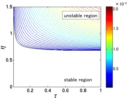
In Figs. 5 and 6, contour plots of the growthrate in the
τandηspace with the H–H model and the reduced gyro-fluid model, respectively, are given. Criticalηc is much
smaller in the case with the H–H model than with the gyro-fluid model. In Fig. 5 the mode is unstable even withη= 0, whenτis greater than 0.6. Figure 6 shows the same level of criticalηcas in Fig. 1 even with this reduced set of
equations, although the dependency onτbecomes weaker. The results differ because of the different origins of the term in each model, i.e., the polarization velocity term in the H–H model, and the gyro-averaging in the gyro-fluid model. In the H–H model, the polarization term can cou-ple with the diamagnetic drift term, which is not included in the gyro-fluid model. Whenωω∗, the analytical
so-Fig. 6 Contour plot of the growthrate in theτandηspace with the reduced gyro-fluid model. This is the case of argon plasma.
lutions become
ω=±kz
τ(1+η)
1−bτ(1+η)−γτ, (22) with the H–H model, and
ω=±kz
1+bτ
2
τη
1−bτη/2− 2 3τ
, (23)
with the reduced gyro-fluid model, whereω∗=kθ/Lnis the diamagnetic drift frequency. Criticalηcis obtained to be
ηc= γ
1+γbτ−1, (24)
with the H–H model, and
ηc=
2
3+bτ, (25)
with the reduced gyro-fluid model. By settingb=0 and usingγ =5/3, the condition for ITG excitationη > 2/3 can be derived from both models.
5. Summary
The excitation condition for the ITG instability in lin-ear device PANTA has been investigated using the gyro-fluid model. Linear stability analyses show the dependen-cies of the linear growthrate on the ion mass, the temper-ature gradient, the magnitude of the FLR effect, and the thermal anisotropy. Although the modenumbers of the most unstable modes differ for different discharge gases, their critical values have almost the same η value, i.e.,
Acknowledgements
Authors acknowledge discussions with Prof. S. Ina-gaki, Dr. M. Sasaki, Dr. Y. Kosuga, and Mr. Y. Miwa. This work is supported by the Grant-in-Aid for Young Scientists (24760703), for Scientific Research (23244113) of JSPS, by the collaboration program of NIFS (NIFS13KNST050, NIFS13KOCT001) and of RIAM of Kyushu University.
[1] P.H. Diamondet al., Plasma Phys. Control. Fusion47, R35 (2005).
[2] W. Horton, Rev. Mod. Phys.71, 735 (1999). [3] B. Coppiet al., Phys. Fluids10, 582 (1967).
[4] G.W. Hammett and F.W. Perkins, Phys. Rev. Lett.64, 3019
(1990).
[5] G.S. Lee and P.H. Diamond, Phys. Fluids29, 3291 (1986). [6] A.K. Senet al., Phys. Rev. Lett.66, 429 (1991).
[7] S. Oldenbürger et al., Plasma Phys. Control. Fusion 54, 055002 (2012).
[8] S. Inagakiet al., Plasma Fusion Res.9, 1201216 (2014). [9] Y. Miwaet al., Plasma Fusion Res.8, 2403133 (2013). [10] W. Dorland and G.W. Hammett, Phys. Fluids B 5, 812
(1993).
[11] P. Snyder, Ph. D. thesis, Princeton Univ. (1999).
[12] S. Hamaguchi and W. Horton, Phys. Fluids B 2, 1833 (1990).
[13] R. Balescu, Aspect of Anomalous Transport in Plasmas