MARKET EFFICIENCY ANALYSIS OF AMMAN STOCK
EXCHANGE THROUGH MOVING AVERAGE METHOD
Sameer Al Barghouthi
Al Falah University
Aysha Ehsan
Al Falah University
ABSTRACT
This paper employs the Moving Average (MA) method which is a technical analysis designed to generate a rule to develop appropriate investment positions at any given time. In context of market index, it works with a comparative analysis of most recent index level (short MA) with the contrary long MA of the index. A short MA (one day) in comparison with long MAs is the focus of this study, in conjunction with ‘zero filter’. The results are compared against the efficient market hypothesis which confirms that if technical analysis has a significant value it is a sign of an inefficient market at weak form. The case study of the five Jordanian indices in the market strengthens the hypothesis as it demonstrates that the application of MA technique allows significant returns as the predictability of the market is enhanced. The market analysis from January 1, 2008 to December 31, 2016 has proven that ASE is inefficient at weak form level thus offering opportunities to traders to make abnormal profits.
Keywords: Technical Trading; Moving Average; ASE; Jordanian Indices.
1. INTRODUCTION
Technical trading analysis has a long history dated back to the turn of last century. The basic concept of technical analysis is to use past prices to predict future stock prices in stock trading. Traders analyse the pattern of past market price data and assume that the trend can recur in the future. By doing this they can predict future prices and make a profit. If traders are able to recognise changes in trend at very early stage they can hold an investment portfolio until that trend changes. This means they can identify the time period to sell or buy stocks. It is very common among securities firms to use technical analysis in their investment strategies. The main reason for securities firms to use technical trading rules is the simplicity of the methodology.
The purpose of this research is to examine the efficiency of Amman Stock Exchange by using technical trading rules, through the analysis of the five Jordanian indices. As the market study is an on-going process and its dynamics keep fluctuating on regular basis, therefore its analysis is vital. This study has taken the results of previous researches made on markets analysis and extended it further to add to the wealth of research and provide opportunities to curtail inequality and corruption in business. This study has filled the gap of the defined time span in Jordanian markets for better understanding of its performance.
Corresponding author: Sameer Al Barghouthi, Al Falah University P.O.Box: 128821 Dubai, UAE, 0097142338080,
In this study five Jordanian indices have been employed because the disclosure of banks is highly different from that of financial markets. In case of banks, the Central Bank sketches the rules which ensure a regulated movement of finances. The case of financial markets is not on the similar lines. As it is free flowing process it offers a huge amount of opportunity to investors. With such abundance of venues the investors need the understanding of the market through the knowledge of its efficiency or inefficiency.
Moreover, this paper compares the results associated with Jordanian General Index to the performance of S&P 500, FTSE 100, and Hang Seng Hong Kong Indices.
2. LITERATURE REVIEW
Early researches such as Fama and Blume (1966) and Jensen and Benington (1970) conclude that technical analysis is not helpful in predicting future market prices.Meese and Rogoff (1983) finds that no economic model is available that could outperform random walk models.
Krishnamurthi and Raj (1988), employing tick data from the Sydney Futures Exchange, concludes that the application of simple trading rules cannot realize abnormal returns. Hudson et al. (1996) adopted the technical trading rules of Brock et al. (1992) and applied it on United Kingdom (UK) stock prices to examine whether trading result is replicable or not in the presence of costly trading environment. They used the daily Financial Times Industrial Ordinary Index from July 1935 to January 1994. The study indicated the predictive ability of technical trading rules but the use of these technical trading rules do not allow investors to make excess returns after taking the transaction costs of 1% per round trip transaction. This is to compare with the average excess returns per round trip transaction of 0.8% from the application of technical trading rules. Ojah and Karemera (1999) document evidence that show that equity prices in major Latin American Emerging equity markets. Argentina, Brazil, Chile and Mexico- follow a random walk, and that they are, generally, weak form efficient.
Elbarghouthi, Qasim, Yassin (2012a), employed test-runs to gauge the efficiency of Amman Stock Exchange. It was proved that the price behavior in ASE does not follow random walk model over time. The ASE reflects a high degree of positive temporal dependency patterns, violating the assumption of random walk model. However, this does not necessarily imply a violation of weak form efficiency. Evidence supporting the random walk model is evidence of market efficiency. But violation of the random walk model need not be evidence of market inefficiency in the weak form.
Coutts and Cheung (2000) investigate the applicability and validity of trading rules in the Hang Seng Index on the Hong Kong Stock Exchange. They find that in terms of implementation of a few technical analysis rules, one would fail to provide positive abnormal returns net of transaction costs, and the associated opportunity costs of investing. Goodacre and Kohn-Speyer (2001) find that once adjustment for market movements and risk are incorporated, technical analysis ceases to be profitable even with an assumption of zero transaction costs.
Lo and MacKinlay (1988, 1999) show, for a weekly U.S. stock indexes that past prices may be used to forecast future returns to some degree, a fact that is the starting point in any technical analysis. Hodrick (1987) and Frankel and Froot (1987) reject the Efficient Market Hypothesis (EMH) in the foreign exchange market. Other studies provide indirect support for technical analysis. These studies include those by Treynor and Ferguson (1985), Brown and Jennings (1989), Jagadeesh and Titman (1993) and Lo and MacKinlay (1999).).
More direct support for technical analysis has been given by De Bondt and Thaler (1985), Brock, Lakonishok, and LeBaron (1992), Jegadeesh and Titman (1993), Bessembinder and Chan (1995), Neely and Weller (1999), Urrutia (1995), Gencay and Sangos (1997), and Allen and Karjalainen (1999).
Some studies have found qualified support for technical analysis. For example, Ratner and Leal (1999) examined the potential profit of a few variable length moving average technical trading rules in ten emerging equity markets in Latin America and Asia from 1982 through 1995. They find that only Taiwan, Thailand and Mexico emerged as markets where technical trading strategies may be profitable.
Al Barghouthi, Rehman, Fahmy and Ehsan (2016) examined the level of efficiency of ASE on all three levels (weak, semi-strong and strong). An analysis of the market performance from 2008 – 2014 concluded that there was significant predictive performance of ASE. The Box-Jenkins estimation was used to prove the results which were confirmed by unit-root test.
A similarly qualified support is found in Szakmary, Davidson and Schwarz (1999) who apply trading rules to Nasdaq stocks. They find that such trading rules conditioned on a stock's past price history perform poorly, but those based on past movements in the overall Nasdaq Index tend to earn statistically significant abnormal returns. However, once they incorporated transaction costs, these abnormal returns are generally not economically significant.
Kampouridis and Otero (2017) have developed the trading strategy that helps amplify profitability in foreign exchange market by using event-based algorithms called Directional Changes. Employing 255 different sets of data in six currencies the event-based analysis opens venues to multiple predictive strategies.
Park and Irwin (2004) investigates the legitimacy of predictability of technical trading analysis by using two stages. Initially studying the results of original study and replicating the same procedure on a new set of data. In the second stage more trading systems and markets are studied by implementing the data-snooping adjusted statistical tests. These tests specifically quantify the results by evaluating the best performing market in the context of technical trading analysis. Through these studies it is derived that trading analysis is not a very string pillar in predicting the future performance of market.
cases of informed trading in contrast to the price crossover rule where the trading rules are better in concentrating significance from a similar price/cost data.
Irwin and Brorsen (1987) studies the uncertainty of technical trading analysis in technical trading system returns. A thorough study of returns from 1978-1984 signified that future funds equity is not an appropriate calculator of technical trading systems. From the results obtained it was observed that technical trading offers help in periods of uncertainty only.
Mishra (2016) uses multiple regression analysis to measure the impact and practicality of technical trading strategies. The extent of trading profitability is further examined in risk compensation for investing in equity markets. This is analyzed by Bollinger Bands (volatility indicators), moving average (trend indicators), Relative Strenght Index (momentum indicator) and Elliot theory (mass psychology indicator). It is proved that technical indicators can be employed while evaluating strategies for investment.
Elbarghouthi, Yasin and Qasim (2012b), analysed the behavioural properties of Amman Stock Exchange (ASE) indices. The Box-Jenkins estimation, irrespective of the index examined produced different models with a high prediction performance, violating the EMH conditions. The unit-root test also confirmed these results since the return series for all indices did not exhibit unit root, and all processes were stationary.
Al Barghouthi , Rehman and Rawashdeh (2016) examined financial integration and the co-movement of stock prices by using cointegration tests. The presence of cointegration relations indicates clear violation of market efficiency as is an indicator of possibility of employing information in past prices to forecast the current and future prices.
3. TECHNICAL TRADING RULES
In this paper we have used the Moving Average technique because this technique engages the contemporary scenario of the time span considered. Many other predictability tools only indicate the statistical results but Moving Average reflects the market performance clearly indicating when the financial market if inefficient and investors are making abnormal profits. According to the moving average rule, buy and sell signals are generated by two moving averages of the level of the index, Two types of moving averages (MA) will be used here. Short and long (MA). The short MA consists of one day (the index itself), while the longer MAs will be based on varying ranges of 2, 4,10,20,50,100 and 150 days, Using no filter, The signal is generated by comparing a short-term moving average of price to a long-term moving average, this strategy is express as buying (or selling) when the short (MA) rises above (or falls below) the long (MA). In this study one day has been used as the short-term moving average. This is to compare with the long-term moving averages of 2 days, 4 days, 5days, 10days 20days, 50 days, 100 days, and 150 days.
The null hypothesis tested in this study is:
Null hypothesis:
H1: The mean returns generated by technical trading rules is not equal to the returns derived by the buy-and-hold strategy
Table (1) contains a summary of the daily returns and its standard deviation for buy-and-hold strategy for the entire full sample. t-statistic test is adopted in order to examine mean differences between each technical trading rule with the strategy of buy-and-hold. This test has been used by some studies like Brock, et al, (1992). The t-statistics for the buys (sells) are:
2 / 1 2 2 ) / / ( r r N N T
Where r and Nr are the mean return and number of signals for the buys and sells, and
and N are the unconditional mean and number of observations. 2is the estimated variance for the entire sample. For the returns difference between buy-sell, the t-statistic is,2 / 1 2 2 ) / /
( b s
s b N N T
Where b and Nb are the mean return and number of signals for the buys and s and Ns are the mean
return and number of signals for the sell
4. PROFIT MEASUREMENT
Two investment strategies are investigated: long-cash and long-short strategies. In the long-cash strategy when a buying signal is received, a long position in the index is initiated, and when a signal to sell is received, the index is sold, and the proceeds are held in cash. In the long-short strategy, in contrast, when a selling signal is received, the index is sold short. The resulting rate of return on each of the two strategies will be compared to the return on a buy-and-hold (BH) policy. That is, the return on the index when held up to the end of the test period. A strategy return higher than the return of the BH policy indicates market inefficiency in the weak form.
Rates of return are computed for each holding period whose length is determined by the signal received from the MA method. The compound rate of return for the whole test period is then compared to the return on the simple BH policy. The specific date of the final signal varies by a few days between the long-cash strategy and the long-short strategy. For the first strategy, it is the date of the final long signal received, while for the second strategy, it is the date of either a long or short signal. That is why the corresponding return on the alternative BH policy may vary a bit between the two strategies, i.e., long-cash and long-short.
The profits of the buy signals are computed as follows:
Profit ( ) = mean return (buy) x trade per year
Profit ( ) = mean return (sell) x trade per year
The technical trading rules are also examined in trading cost environment. The method of computation of breakeven transaction costs is used by Bessembinder and Chan (1995). The percentage round trip transaction cost is denoted as C. When a buy or sell signal is emitted, the C/2 transaction cost will be deducted from the return. Another C/2 will be charged when the position is closed out. Consequently, the breakeven transaction costs are:
s b N
N C
Nb = Number of days in which a buy signal is generated in a year Ns = Number of days in which a sell signal is generated in a year C = Percentage round trip transaction costs
= Profit generated from technical trading rules as compared to buy-and-hold strategyRearranging the above equation, the profit derived from applying the technical trading rules is given as follows:
= Total
(before transaction cost) - C * (Nb + Ns).In addition to the cost of the shares bought or sold, the investor will have to pay the transaction costs in Jordan. The percentage transaction cost in Jordan is 0.8% for the buy transaction and 0.65 % for the sell transaction.
5. DATA
This research has been conducted to performance of ASE by analyzing the daily index prices of five Jordanian indices from 1-1-2008 to 31-12-2016.
Table 1: The Mean Returns and the Standard Deviation for the Jordanian and the International Markets Indices
Index Bank Services Insurance Industry General S&P500 Heng Seng Ftse100
N 2236 2425 2425 2425 2425 2425 2425 2425
Mean 0.00009919 -0.00021 -0.00016 -0.00038 -9.6E-05 0.000561 0.000115 0.000312
Std 0.67613 0.62153 0.366639 0.721994 0.558103 0.9191 1.79543 0.89635
Table 2: MA results for the Bank index
Rule N(Buy) N(Sell) Buy Sell Buy-Sell
(1,2) 1005 1177 0.001313 -0.0009 0.002213 26.87% -156.53%
(3.7647)1 (-3.4032)1 (7.1679)2
(1,4) 1012 1174 0.003715 -0.00291 0.006625 80.21% -150.06%
(11.2501) (-9.9849) (21.235)
(1,5) 983 1202 0.00361 -0.00291 0.00652 82.44% -151.26%
(11.8540) (-10.0772) (21.9312)
(1,10) 989 1191 0.003028 -0.00226 0.005288 63.40% -152.26%
Table 2: MA results for the Bank index (cont.)
Rule N(Buy) N(Sell) Buy Sell Buy-Sell
(1,20) 1017 1153 0.00218 -0.00174 0.0039 47.16% -152.14%
(6.4898) (-6.0629) (12.5527)
(1,50) 1009 1131 0.001553 -0.00125 0.002803 33.11% -150.85%
(4.5164) (-4.4023) (8.9187)
(1,100) 1186 1140 0.001232 -0.00080 0.002032 22.99% -147.36%
(3.4259) (-2.9673) (6.3932)
(1,150) 1020 1020 0.00168 -0.00086 0.00254 21.86% -132.20%
(3.0642) (-3.3030) (6.3672)
Average 0.002289 -0.00170 0.003990
Notes:1The T-statistic ratio that tests the mean returns generated by technical trading rules equal to the returns derived by the buy-and-hold strategy. All the third rows of the each test present t-statistic ratios in parentheses; 2 The t-statistic ratio of return buy-sell differences;N(Buy) refers to the number of buy signals generated during the sample period; N(Sell) refers to the number of sell signals generated during the sample period; refers to the average annual profit before transaction cost; refers to the average annual profit after transaction cost; Hold and Buy strategy Annual return = 2.86%.
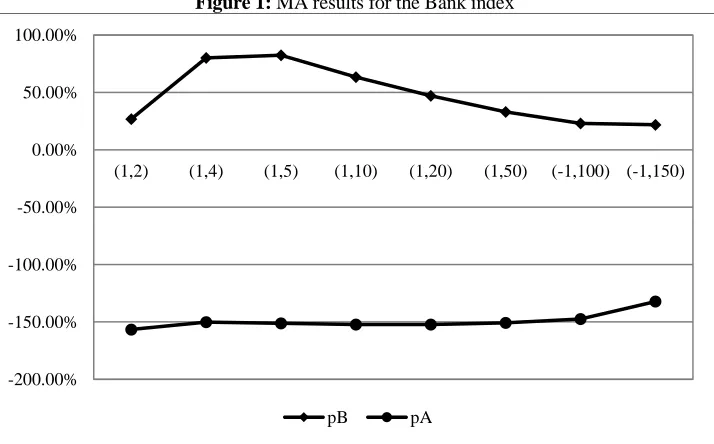
Figure 1: MA results for the Bank index
Table (2) shows that the buy returns of the bank index are positive with an average of 0.002289, which outperform the unconditional return of the bank index estimated at 0.000109 (see table 1). All the rules that have been tested rejected the null hypothesis that the return equals the unconditional return at the 1 and 5 % level. For sell signals all the test results rejected the null hypothesis in which the MA rules gain the same return as the buy-and-hold strategy. The buy-sell differences show the highly positive return which has been gained by adopting the MA rules and shows highly significance at the level of 5%. The profit (B) column indicates, positive average annual return before taken into consideration the transaction cost which outperforms the unconditional return for the whole bank sample. This confirms the previous results of the inefficiency at weak form level of the bank sector. However, the annual average return does not outperform the unconditional return once the transaction cost is taken into consideration.
-200.00% -150.00% -100.00% -50.00% 0.00% 50.00% 100.00%
(1,2) (1,4) (1,5) (1,10) (1,20) (1,50) (-1,100) (-1,150)
Table 3: MA Results for the service index
Rule N(Buy) N(Sell) Buy Sell Buy-Sell
(1,2) 1010 1156 0.00074 -0.00102 0.00176 21.76% -155.49%
(3.2402) (-2.9265) (6.1667)
(1,4) 957 1227 0.003400 -0.0028 0.0062 75.10% -153.16%
(11.9123) (-9.6208) (21.5331)
(1,5) 947 1238 0.003429 -0.00280 0.006229 74.87% -153.84%
(11.9461) (-9.5284) (21.4745)
(1,10) 928 1252 0.002721 -0.00224 0.004961 59.54% -154.86%
(9.5324) (-7.5436) (17.076)
(1,20) 924 1246 0.00207 -0.00178 0.00385 46.17% - 154.86%
(7.4016) (-5.8311) (13.2327)
(1,50) 880 1260 0.00129 -0.00121 0.0025 29.66% -152.46%
(4.7698) (-3.7209) (8.4907)
(1,100) 766 1324 0.001180 -0.00089 0.00207 22.78% -147.69%
(4.4095) (-2.5738) (6.9833)
(1,150) 707 1333 0.000820 -0.00064 0.00146 15.64% -142.35%
(2.8991) (-1.6547) (4.5538)
Average 0.001956 -0.00167 0.006328
Notes: 1The T-statistic ratio that tests the mean returns generated by technical trading rules equal to the returns derived by the buy-and-hold strategy. All the third rows of the each test present t-statistic ratios in parentheses; 2 The t-statistic ratio of return buy-sell differences; N(Buy) refers to the number of buy signals generated during the sample period; N(Sell) refers to the number of sell signals generated during the sample period; refers to the average annual profit before transaction cost; refers to the average annual profit after transaction cost; Hold and Buy strategy Annual return =- 6.05 %.
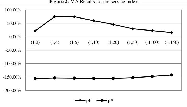
Figure 2: MA Results for the service index
Table 3 reports the results of the t-statistic test for the services index. The results reject the null hypothesis of equality between the unconditional mean return in all rules with the mean return of the service index across the rules except in one case where the t-test is significant at 5% level. This significance is seen in the sell mean return associated with the rule (1-150). However, the t-test of the buy-sell mean return associated with the same rule is insignificant. The results indicate that the service
-200.00% -150.00% -100.00% -50.00% 0.00% 50.00% 100.00%
(1,2) (1,4) (1,5) (1,10) (1,20) (1,50) (-1100) (-1150)
sector in ASE is inefficient at weak form level as the investor can make abnormal profits by using the past prices.
Table 4: MA results for the insurance index
Rule N(Buy) N(Sell) Buy Sell Buy-Sell
(1,2) 751 896 0.000405 -0.00049 0.00089 7.15% -106.86%
(2.7760) (-1.5507) (4.3267)
(1,4) 929 1124 0.001595 -0.00154 0.003135 35.33% -141.30%
(9.6620) (-8.3066) (15.3529)
(1,5) 953 1161 0.00148 -0.00144 0.00292 34.31% -148.30%
(9.1959) (-7.8128) (17.0087)
(1,10) 926 1254 0.001329 -0.0011 0.002429 30.34% -156.55%
(8.1863) (-6.4500) (14.6363)
(1,20) 871 1299 0.001101 -0.00092 0.002021 24.04% -155.98%
(6.7247) (-4.8847) (11.6094)
(1,50) 864 1278 0.00062 -0.00629 0.00691 15.04% -153.09%
(3.4697) (-3.00265) (6.4723)
(1,100) 809 1281 0.000517 -0.00046 0.000977 11.25% -147.97%
(2.6682) (-1.9774) (4.6456)
(1,150) 683 1357 0.000414 -0.00032 0.000734 7.906% -141.92%
(2.8991) (-1.10726) (4.0063)
Average 0.009326 -0.00157 0.002502
Notes: 1The T-statistic ratio that tests the mean returns generated by technical trading rules equal to the returns derived by the buy-and-hold strategy. All the third rows of the each test present t-statistic ratios in parentheses. 2 The t-statistic ratio of return buy-sell differences.N(Buy) refers to the number of buy signals generated during the sample period.N(Sell) refers to the number of sell signals generated during the sample period.refers to the average annual profit before transaction cost;
refers to the average annual profit after transaction cost. Hold and Buy strategy Annual return = -4.51%
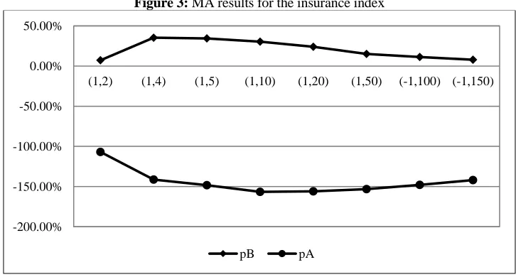
Figure 3: MA results for the insurance index
Table 4 shows that the sell return for the rules (1,2) and (1.150) fail to reject the null hypothesis that the mean return of the insurance sectors equal to the unconditional return. However, the buy-sell mean returns for the same rules reject the null hypothesis. By adopting the MA technique the investors
-200.00% -150.00% -100.00% -50.00% 0.00% 50.00%
(1,2) (1,4) (1,5) (1,10) (1,20) (1,50) (-1,100) (-1,150)
were able to outperform the unconditional return. On the other hand, after taken into consideration the transaction cost the investors fail to outperform the unconditional mean return in question. this indicate that the insurance sector in ASE is inefficient at weak form level.
Table 5: MA results for the Industry index
Rule N(Buy) N(Sell) Buy Sell Buy-Sell
(1,2) 978 1205 0.001379 -0.00175 0.003129 39.01% -155.58%
(5.0644) (-4.2985) (9.3629)
(1,4) 926 1260 0.003997 -0.00334 0.007337 88.33% -154.38%
(12.2651) (-9.4437) (21.7088)
(1,5) 925 1260 0.003999 -0.00333 0.007329 88.28% -154.27%
(12.2569) (-9.4411) (21.698)
(1,10) 862 1318 0.002721 -0.00266 0.005381 72.47% -157.30%
(10.4955) (-7.3914) (17.8869)
(1,20) 853 1317 0.002407 -0.00212 0.004527 56.15% -156.15%
(8.1214) (-5.6606) (13.782)
(1,50) 777 1363 0.001846 -0.00148 0.003326 38.17% -153.68%
(5.7072) (-3.6113) (9.3185)
(1,100) 728 1362 0.001200 -0.00103 0.0023 25.05% -147.86%
(3.9107) (-2.1210) (6.0317)
(1,150) 678 1362 0.00105 -0.00093 0.00198 21.73% -142.49%
(3.4133) (-1.8067) (5.22)
Average 0.002324 -0.00208 0.004413
Notes:1The T-statistic ratio that tests the mean returns generated by technical trading rules equal to the returns derived by the buy-and-hold strategy. All the third rows of the each test present t-statistic ratios in parentheses.2 The t-statistic ratio of return buy-sell differences.N(Buy) refers to the number of buy signals generated during the sample period.N(Sell) refers to the number of sell signals generated during the sample period. refers to the average annual profit before transaction cost;
refers to the average annual profit after transaction cost. Hold and Buy strategy Annual return = - 11.22 %
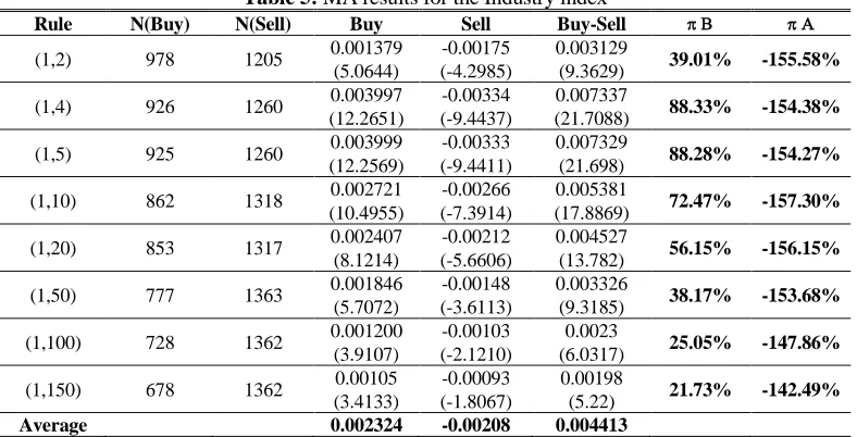
Figure 4: MA results for the Industry index
-200.00% -150.00% -100.00% -50.00% 0.00% 50.00% 100.00% 150.00%
(1,2) (1,4) (1,5) (1,10) (1,20) (1,50) (-1,100) (-1,150)
Table 5 displays that the t-test of all the rules reject the null hypothesis at 1 and 5 % levels. The positive average annual profit before taken into consideration the transaction cost outperform the unconditional return but after including the transaction action the average annual return could not outperform the unconditional return. This result indicates that the industry sector in ASE is inefficient at weak form level.
Table 6: MA results for the Industry index
Rule N(Buy) N(Sell) Buy Sell Buy-Sell
(1,2) 1000 1185 0.00119 -0.00116 0.00235 28.88% -156.19%
(4.830496) (-4.33330) (9.1642)
(1,4) 969 1216 0.003287 -0.00263 0.005917 71.37% -153.05%
(12.50515) (-10.3576) (22.8627)
(1,5) 971 1214 0.003347 -0.00270 0.00604 72.90% -152.82%
(12.7401) (-10.6063) (23.3464)
(1,10) 942 1238 0.002614 -0.00224 0.004854 55.67% -154.65%
(98859) (-8.7672) (98867)
(1,20) 985 1185 0.00195 -0.00176 0.00371 44.75% -153.20%
(7.6295) (-6.7069) (14.3364)
(1,50) 935 1205 0.001284 -0.00115 0.002434 28.81% -152.11%
(5.0185) (-4.2953) (9.3138)
(1,100) 881 1209 0.00093 -0.00076 0.00169 19.32% -147.84%
(3.6586) (-2.7259) (6.3845)
(1,150) 923 1117 0.000747 -0.00073 0.001477 16.61% -143.27%
(3.0459) (-2.5247) (5.5706)
Average 0.001918 -0.00131 0.003559
Notes: 1The T-statistic ratio that tests the mean returns generated by technical trading rules equal to the returns derived by the buy-and-hold strategy. All the third rows of the each test present t-statistic ratios in parentheses.2 The t-statistic ratio of return buy-sell differences.N(Buy) refers to the number of buy signals generated during the sample period.N(Sell) refers to the number of sell signals generated during the sample period.refers to the average annual profit before transaction cost;
refers to the average annual profit after transaction cost. Hold and Buy strategy Annual return = -2.75 %
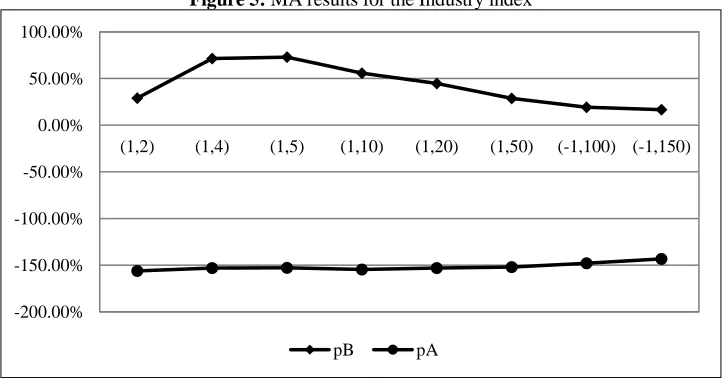
Figure 5: MA results for the Industry index
-200.00% -150.00% -100.00% -50.00% 0.00% 50.00% 100.00%
(1,2) (1,4) (1,5) (1,10) (1,20) (1,50) (-1,100) (-1,150)
Also table 6 shows that the average annual profits for all the rules before including the transaction cost outperform the buy and hold strategy (unconditional return). On the other hand, the average annual profits do not outperform the unconditional return once the transaction cost is included.
Table 7: Comparison between ASE and other International Market S&P500
FSTE
Hong Kong General index
S&P500 FSTE
Hong Kong General index
Rule (1,2) (1,2) (1,2) (1,2)
No buys 1167 1140 1114 1000
Mean (Buy) 0.000432 0.000624 8.31E-05 0.001191
(-0.31834) (0.765617) (-0.00392) (4.83058)
No sells 1020 1041 1073 1185
Mean (Sell) 0.000734 -4.01E-05 6.67E-05 -0.00116
(0.393330) ( -0.84133) (-0.05825) ( -4.33330)
Buy - Sell -0.000302 4.010624 1.64E-05 0.00351
(-0.71167) (1.606947) (0.05433) (9.16388)
Table (7) reports the results generated by using MA for the rule (1, 2) for the three international stock market indices and the Jordanian general index. The results for the three international stock markets fail to reject the null hypothesis that The mean returns generated by technical trading rules equals the returns generated by the buy-and-hold strategy unlike the result that concerns the Jordanian General index which, rejects the null hypothesis. The results indicated that by adopting the Moving average technique for the rule (1,2), the investors could not outperform any of the three international stock markets, hence, making abnormal profit. The results indicate that the three international stock markets are efficient at weak form level while the Jordanian general index is inefficient at weak form level.
6. RESULT
The results of the study show that transparency in financial market is a key to enhanced trading and influx of investors. An efficient market attracts better business and serious investors. This gives rise to investor confidence, liquidity and better trading. The study has directed to policies that lead to bringing transparency in financial markets (Antoniou, Ergul, and Holmes (1997)) and offered insight in coping with inadequacies that lead to an inefficient market.
7. DISCUSSION
The results of this paper support the previous research carried out on ASE, “The use of unit root and Box-Jenkins in Amman Stock Exchange (ASE)” (2016) and “Testing the Efficiency of ASE by the Two Step Regression Based Technique, the Johansen Multivariate Technique Cointegration, and Granger Causality” (2016), proving that ASE is inefficient at weak form level. ASE therefore produces predictable profits thus offering traders the opportunities to make abnormal profits.
cost is included the investors in the ASE could not outperform the buy and hold strategy and could not achieve abnormal profits. Consequently it appears that the transaction cost prevented the investors to achieve abnormal profits, which made the ASE efficient at weak form level. This implies that the higher the transaction cost is, the more efficient the stock market will be. This logic contradicts the views of prominent scholars in the field like Fama who states that the absence of the transaction cost is one of the sufficient conditions of the efficiency of the stock markets. Most importantly the finding related to the transaction cost imply that the efficiency of ASE did not reflect the fairness of the Jordanian stock market which contradict the core purpose of the concept of the efficient market hypothesis that the market is a fair game where the shares prices reflect their true value, and where the investors do not achieve abnormal profits at the expenses of the other investors.
REFERENCES
Al Barghouthi, S., Rehman, I. U., & Rawashdeh, G. (2016). Testing the Efficiency of ASE by the Two Step Regression Based Technique, the Johansen Multivariate Technique Cointegration, and Granger Causality. Electronic Journal of Applied Statistical Analysis, 9(3), 572-586. Al Barghouthi, S., Rehman, I., Fahmy, S., & Ehsan, A. (2016). The use of unit root and Box-Jenkins in
Amman Stock Exchange (ASE). ElectronicJournal of Applied Statistical Analysis, 9(3), 552-571. Allen, F., & Karjalainen, R. (1999). Using Genetic Algorithms to Find Technical Trading Rules.
Journal of Financial Economics, 51(2), 245-271.
Antoniou, A., Ergul, N., & Holmes, P. (1997). Market Efficiency, Thin Trading, and Non-linear Behaviour; Evidence from an Emerging Market. European Financial Management, 3(2), 175-190.
Bessembinder, H., & Chan, K. (1995). The profitability of technical trading rules in the Asian stock markets. Pacific-Basin Finance Journal, 3(2–3), 257-284.
Brock, W., Lakonishok, J., & Lebanon, B. (1992). Simple Technical Trading Rules and the Stochastic Properties of Stock Returns. Journal of Finance, 47(5), 1731-1764.
Brown, D. P., & Jennings, R. H. (1989). On Technical Analysis. The Review of Financial Studies, 2(4), 527–551.
Coutts, A., & Cheung, K. (2000). Trading Rules and Stock Returns: Some Preliminary Short Run Evidence from the Hang Seng1985-1997. Applied Financial Economics, 10(6), 579-586. De Bondt, W. F. M., & Thaler, R. H. (1995). Financial decision-making in markets and firms: A
behavioral perspective, Handbooks in Operations Research and Management Science, Elsevier,9, 385-410.
Elbarghouthi, S., Yassin, M., & Qasim, A. (2012a). The Use of Runs Test in Amman Stock Exchange. International Business Research,5(2), 159-172.
Elbarghouthi, S., Yassin, M., & Qasim, A. (2012b). Is Amman Stock Exchange an Efficient Market? International Business Research, 5(1), 140-156.
Fama, E., & Blume, M. (1966). Filter Rules and Stock Market Trading Profits. Journal of Business, 39(1), 226-241.
Frankel, J. A., & Froot, K. A. (1987). Short-term and long-term expectations of the yen/dollar exchange rate: Evidence from survey data. Journal of the Japanese and International Economies, 1(3), 249-274.
Gencay, R., & Sangos, T. (1997). Technical Trading Rule and the Size of the Risk Premium in Security Reruns. Studies in Nonlinear Dynamics and Econometrics,2, 23-34.
Hodrick, R. J., & Srivastava, S. (1996). Foreign currency futures. Journal of International Economics, 22(1–2), 1987, 1-24.
Hudson, R., Dempsey, M., & Keasey, K. (1996). A Note on the Weak Form Efficiency of Capital Markets: The Application of Simple Technical Trading Rules to UK stock prices- 1935 to 1994. Journal of Banking and Finance, 20(6), 1121- 1132.
Irwin, S. H., & Brorsen, B. W. (1987). A note on the factors affecting technical trading system returns. The Journal of Futures Markets,7(5), 591-595.
Jegadeesh, N., & Titman, S. (1993). Returns to Buying Winners and Selling Losers: Implications for Stock Market Efficiency. The Journal of Finance, 48(1), 65-91.
Jensen, M., & Benington, G. (1970). Random Walk and Technical Theories: Some Additional Evidence. Journal of Finance, 25(2), 469-482.
Kampouridis, M., & Otero, F. E. B. (2017). Evolving trading strategies using directional changes. Expert Systems with Application, 73, 145-160.
Krishnamurthi, L., & Raj. S. P (1988). A Model of Brand Choice and Purchase Quantity Price Sensitivities, Marketing Science, 7(1), 1-20.
Lo, A. W., Mamaysky, H., & Wang, J. (2000). Foundations of Technical Analysis: Computational Algorithms, Statistical Inference, and Empirical Implementation. The Journal of Finance, 55(4), 1705-1765.
Lo, A., & MacKinlay, A. (1988). Stock Market Prices Do Not Follow Random Walks: Evidence from a Simple Specification Test. Review of Financial Studies, 1(1), 41-66.
Lo, A., & MacKinlay, A. (1999). A Non Random Walk down Wall Street. Princeton: Princeton University Press.
Meese, R. A., & Rogoff, K. (1983). Empirical exchange rate models of the seventies: Do they fit out of sample? Journal of International Economics, 14(1–2), 3-24.
Mishra, S. (2016). Technical analysis and risk premium in indian equity market: A multiple regression analysis. IUP Journal of Applied Economics, 15(1), 51-68.
Neely, C., & Weller, P. (1999). Technical Trading Rules in the European Monetary System. Journal of International Money and Finance, 18(3), 429-458.
Ojah, K., & Karemera, D. (1999). Random Walks and Market Efficiency Tests of Latin American Emerging Equity Markets: A Revisit. Financial Review, 34(2), 57-72.
Park, C-H., & Irwin, S. H. (2004). The profitability of technical trading rules in United States futures markets: A Data Snooping Free Test. Paper presented at the NCR-134 Conference on Applied Commodity Price Analysis, Forecasting, and Market Risk Management, St. Louis, Missouri. Ratner, M., & Leal, R. (1999). Tests of Technical Trading Strategies in the Emerging Equity Markets
of Latin America and Asia. Journal of Banking and Finance, 23(12), 1887-1905.
Szakmary, A., Davidson, N., & Schwarz, T. (1999). Filter Tests in NASDAQ Stocks. Financial Review, 34(1), 45-70.
Toms, M. C. (2011). The technical analysis method of moving average trading: Rules that reduce the number of losing trades (Unpublished doctoral dissertation). Newcastle University, Newcastle upon Tyne, United Kingdom.
Treynor, J. L., & Ferguson, R. (1985). In Defense of Technical Analysis. The Journal of Finance, 40(3), 757-773.