Published online February 20, 2013 (http://www.sciencepublishinggroup.com/j/acis) doi: 10.11648/j. acis.20130101.12
Robust generalized minimum variance controller using
neural network for civil engineering problems
L. Guenfaf
1,*, M. Djebiri
2, M. S. Boucherit
2, F. Boudjema
21LSEI Laboratory, USTHB University BP 32 El Alia 16111, Bab Ezzouar, Algiers, Algeria 2LCP, Laboratory, ENP, Hassan Badi El harrach, Algiers, Algeria
Email address:
[email protected] (L. Guenfaf)
To cite this article:
L. Guenfaf, M. Djebiri, M. S, Boucherit, F. Boudjema. Robust Generalized Minimum Variance Controller Using Neural Network for Civil Engineering Problems, Automation, Control and Intelligent Systems. Vol. 1, No. 1, 2013, pp. 7-15.
doi: 10.11648/j.acis.20130101.12
Abstract:
This paper presents a robustness of the proposed generalized minimum variance algorithm. The main idea is to use artificial neural network for generalization of the GMV. This will give a neural network-based control method wich can be applied to civil engineering structures. The neural network learns the control task from an already existing controller, which is the generalized minimum variance (GMV) controller. The objective is to take advantage of the generalization capabilities and the nonlinear behavior of neural networks in order to overcome the limitations of the existing controller and even to improve its performances. Simulation results demonstrate the robustness of this algorithm and its capability to compensate the structural parameter variations and seismic ground motion.Keywords:
Structural Control, Neural Networks, Generalized Minimum Variance Control1. Introduction
Structural control is an expanding field of study since the increasing need to save human being lives and reduce structural damage [18]. For this purpose, many active con-trol techniques have been investigated and applied to structural systems in order to reduce their dynamic response under earthquake excitation. But most of these techniques suffer one or more of the following disadvantages: (1) the control law is usually designed assuming a linear or a li-nearized behavior around a desired state of the structure being controlled, (2) structural parameters are supposed to remain constant along all the control time history, i.e., the structure suffers no damage or deterioration, (3) the control is designed for a specific type of earthquake excitation. If the above mentioned statements are verified, control efficiency will be ensured in most cases. However, in practical situa-tions structures may exhibit a nonlinear behavior caused either by large displacements or material nonlinearity and damage. In other hand, structural model uncertainties and parameter variations, especially under severe earthquakes, are very probably to occur. These practical considerations will limit the effectiveness of the control system and per-formances of the control technique will be severely affected.
Faced with this kind of problems, civil engineers have turned to a more powerful tool which can perform control
actions while compensating for unpredictable environmental changes. Neural networks have demonstrated their abilities to accomplish this task. They become a challenging alter-native to solve specific structural problems, handling their attractive features such as nonlinearity, parallel processing, learning and generalization capabilities. The ability of neural networks to approximate arbitrary nonlinear map-pings makes them of great deal in control of nonlinear systems.
to nonlinear structural control problems. They demonstrated that the nonlinearly trained neuro-controller was able to reduce the structural damage more than the linearly trained neuro-controller, but globally the two controllers have comparable performances.
In [4] the authors are interested to minimize the norm of the nominal control sensivity transfer function in the condi-tion of non minimum phase system. The stochastic poly-nomial C is chosen by the authors and equal to one in the case study of the paper. Also in an other paper [5] the con-troller is calculated using the variance of the output with and without tracking polynomial. The chosen parameter con-troller is done according to the norm of the output in optimal and suboptimal cases. Whereas Grimble [17] develop the non linear generalized minimum variance for MIMO sys-tems in general case without specification on the parameter variations. Also nonlinear smith predictor is used for im-plementation in the case of open loop stable systems. The authors in [19] present the generalized minimum variance for noisy free systems and STR algorithm for AR systems. The polynomial C is then chosen by the authors. In our approach we are interested to maintain the stochastic beha-vior of the system charatirized by soil structure interaction. The closed loop polynomial is the same as that one of the exogen input to insure the optimal parameter of the con-troller. By using the neural network, we introduce the sto-chastic behavior in the non linear new model. This one can occurs in the generalized case by operating in the non training data.
In this paper, we first investigate the so-called generalized Minimum Variance (GMV) algorithm for buildings under earthquake excitation. The GMV algorithm attempts, by using a certain model of the system to be controlled and its perturbations, to minimize a generalized cost function in-cluding output variance and control effort. The GMV algo-rithm has been widely studied in literature [8,9,14] and has demonstrated good tracking and regulation performances. But these performances, as we will see, are closely related the knowledge of the ARMAX (Auto-Regressive Moving Average eXogen) model of the system to be controlled since the control strategy is derived in the base of this model. Therefore if the ARMAX model changes by changing the seismic excitation model or by structural parameter varia-tions, control performances may be questionable. In the classical control theory we can use the adaptive approach witch need more time calculation and fast sampling time.
To overcome this problem, we will investigate, in this approach, the use of a neural network that learns to control a single-degree-of-freedom (SDOF) structural building from the GMV controller. The neural network controller will acquire control skills from the GMV controller in one hand, Iin the other hand it will use the generalization capabilities of neural networks to overcome the model-based restrictions of the GMV control technique mentioned above. We have tested the robustness of the resulted algorithm against pa-rameter variation of the model. It has also been showed that the seismic exciataion has been taken in charge by the
pro-posed algorithm with out any change in the parameter of the exogen model.
The approach is to avoid the development of robust con-troller with complicated calculation. The idea is to use neural ANN to have a profit of the generalization behviour and parameter variation. We will see that the presented controller can maintain the closed loop performances more that the classical GMV. The robustness is inside the ANN that gives us more unknow information that we have not taken into consideration in the development of the control law. But changing the excitation signal, we are changing the parameter of the polynomial C which affect the closed loop performances. The main result that we are not using an adaptive algorithm which take much calculation time against our algorithm.
2. Dynamical Model of the Structure
In this section, we are interested in formulating the dy-namical equations of motion of a single-degree-of-freedom structure under seismic excitation. where mechanical actu-ators are active tendons. In order to establish the dynamical model, the following assumptions are considered [10]:
1. the structure is supposed to be a lumped mass m in the girder
2. the two vertical axes are weightless and inextensible in the vertical direction with spring constant k/2 each.
After calculation we can Easily derive the dynamical model of the structure[13]:
) ( ) ( ) ( ) ( )
(t cxt kxt ut mx t x
mɺɺ + ɺ + = − ɺɺg (1) where u(t) is the external control force.
m is the structural mass;
c is the internal viscous damping of the structure; k is the elastic stiffness;
x(t) is the relative displacement;
xt(t) is the absolute displacement defined as xg(t) is the ground motion;
) (t xɺg ɺ
represents the ground acceleration.
This model will be used for testing the proposed algo-rithm. The parameter of this one is presented in the next sections of this paper.
We can see that the variation of the mass affect directly the model of the system whereas the seismic excitation do not.
3. ARMAX Model of the Structure
this disturbance is a stationary Gaussian process with ra-tional spectral density.
The calculation of the ARMAX model of the structure under seismic excitation can be done using equation of motion (1). After dividing this equation by m and introduc-ing the notations
m k
=
2 0
ω natural frequency
0
2 ω
ξ
m c
= damping ratio
Equation (1) becomes:
( )
( )
( )
u( )
t x( )
t m t x t x txɺ ɺ ɺɺg
ɺ +2 + 2 = 1 −
0
0 ω
ξω (2)
Now applying Laplace transform to equation (2), we ob-tain
( )
( )
X( )
ss s s U s s m s
X ɺɺg
2 0 0 2 2 0 0 2 2 1 2 1 ω ξω ω ξω + − + + +
= (3)
where X
( )
s ,Xg( )
sɺ ɺ
and U( )s are the Laplace transform
of x
( )
t ,xɺɺg( )
t and u( )
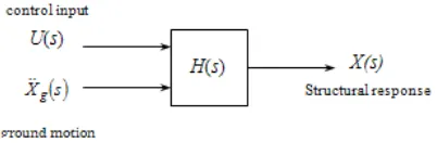
t respectively; s is the Laplace oper-ator. Figure 1 shows the bloc diagram of the structural modelFigure 1. Bloc diagram of the structural model.
The ARMAX model of the structure is obtained by dis-cretization of equation (3). We obtain [15,12]:
( )
( )
( )
( )
( )
( )
x( )
t q A q C t u q A q B tx 1 ɺɺg
1 1 1 − − − − +
= (4)
where
2 2 1 1 1) 1
(q− = +a q− +aq−
A 2 2 1 1 1)
(q− =bq− +b q− B 2 2 1 1 1)
(q− =cq− +c q− C
1 −
q shift operator defined as q−1y
( ) ( )
t+1 =ytThe ground acceleration is described by the Kanai-Tajimi model, i.e
( )
s G sE( )
s Xg = 1( )ɺ ɺ
(5)
Where
( )
2 2 21 1 1 2 2 ) ( ) ( g g g g g g D N s s s s G s G s G ω ω ξ ω ω ξ + + + = =
E(s) is the Laplace transform of white noise.
Discretization of equation (5) gives the discrete ARMAX model of the structure under the Kanai-Tajimi ground ac-celeration. We can see that the parameter of the polynomial C depend directly on those of the structure. The main result here is the excitation signal in the model. So when we change the seismic ground motion, the final model will change as parameter variation. This affects directly the parameter of the exogen input represented by the polynomial C.
4. Generalized Minimum Variance
Controller
The Generalized Minimum Variance (GMV) algorithm was introduced by Clarke [8,9] to control non-minimum phase systems. It is an extension of the Minimum Variance algorithm [1,2] which, by choosing a certain performance criterion, attempts to minimize the variance of the output.
The ARMAX (Auto-Regressive Moving Average eXogen) model of the system is used
( )
t q Bq u( )
t Cq e( )
t yq
A( −1) = −d ( −1) + ( −1) (6) where n nq a q a q
A − = + −1+…+ −
1 1 1 ) ( m mq b q b q
B − = −1+…+ −
1 1 ) ( l lq c q c q
C( −1)=1+ 1 −1+…+ −
noted A, B and C 0
≥
d is the time delay of the system y(t) process output
u(t) control
e(t) white noise with zero mean and of variance σ2. The polynomial C is stable.
The performance index to be minimized is
(
)
(
)
(
)
(
( )
)
[
2 2]
' 1
1 R wt d Qut d
t Py E
J= + + − w + + + (7)
where
E mathematical esperance
(
t+d+1)
w reference signal
)
(q−1
P ,R (q−1)
w and ( )
1
− ′ q
Q weighing polynomials with
) ( ) ( ) ( 1 1 1 − − − = q P q P q P D N and ) ( ' ) ( ' ) ( ' 1 1 1 − − − = q Q q Q q Q D N .
( )
(
(
)
)
( )
QC S P t Ry d t w CR P t u D w D + − + += 1 (8)
Where ) ( ) ( 1 1 1 0 0 0 0 − − ′ ′ ′
= Q q
b p q p q q Q N D D N 0 0 0
0 , D , D and N
N q p p
q′ ′ are the first coefficients of the
polynomials QN′ ,QD′ ,PDandPN respectively.
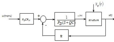
Figure. 2. Generalized Minimum Variance Control architecture.
It is seen from the previous equations that the perfor-mance of the GMV control is closely related to the accuracy of the ARMAX model of the system to be controlled. Therefore, if the ARMAX model used to derive the control law differs from the true ARMAX model of the system, control objectives will not be guaranteed. This can be the case in practical situations where structural parameters change if the building undergo damage or deterioration. Also, if the GMV algorithm is initially designed for a spe-cific model and magnitude of the seismic excitation, its ability to reduce the structural response for a different ex-citation model is uncertain.
The calculation of the control depends on the polynomial C. This polynomial corresponds to the dynamical model as we can see in the Diophantine equation.
4.1. Closed Loop Analysis
To evaluate the regulator performances, we have to cal-culate the closed loop transfer function. From equations 8 and 6 we obtain
( )
( )
e( )
t P S P t w P R P t y N D N wD + '
= (9)
The difference between the output and the obtained model is a noise defined as
( )
e( )
tP S P t N D ' 1 =
ξ (10)
Let ) ( 1 ' ' ' ' ' 1 0 d n D D D D
D P S P P q P nd d q d
P − − +
+ + + + = = … .
Equation (10) becomes
( )
( )
( )
− + − − =∑
∑
+ = = d n i D n i N N D i Ni t i P et i
P P t 0 1 1 1 ' 1 0 ξ
ξ (11)
then
( )
[ ]
− ≤∑
∑
+ = − = d n i D n i N N D i N i P P P t E 0 2 2 1 1 2 2 2 1 ' 1 1 0 σξ (12)
if 0 1 1 1 2 2 0 > −
∑
= N i n i N N P PIn this case, we have evaluated the maximum of the out-put variance, which is the closed loop performance (in the stochastic sense). The closed loop transfer function (be-tween the output and the reference w(t)) is
( )
N w D BF P R P qF −1 = (13)
So the choice of weighing polynomials P and Rw define the reference model. The optimal control is achieved by choosing the closed loop dynamic as C polynome.
5. The Neural Network Controller
The Unlike the conventional control algorithms where the control task is formulated explicitly, in the neural net-work-based structural control methods the neurocontroller learns the control task. The neurocontroller acquires the knowledge of structural control from a set of training cases or an existing controller and stores it in the connection weights[23].
The aim of this section is to use a neural network that replaces the GMV control algorithm. The neural network learns control actions from data generated when the GMV algorithm is controlling the structural system. By using its learning and generalization capabilities the neural network will attempt to perform well and to overcome some of the restrictions of the GMV algorithm.
The overall control is implemented in two stages: 1. Training stage (1): in this stage, the neural network
learns the function input/output of the GMV con-troller. When this later controls the structural system, training examples are generated. Then a supervised learning algorithm is used in order to train the neural network.
Figure 3. The neural network-based control.
5.1. Training Algorithm
The neural network training method used in this study is the well-known Backpropagation algorithm. It is based on the minimization of a quadratic cost function of the error between the desired output and the neural network output. This is done by continuously changing the neural network weights in the direction of the steepest descent of the error cost function.
The output of a unit in the output or hidden layer Oj is given by the following equation:
(
)
∑
= =
i i ji j
j j
O w net
net f O
(14)
where
netj is the weighted sum of the outputs of the previous layer
wji is the connection weight between the i th
node of the previous layer and the jth node of the present layer
f(.) denotes the activation function of the nodes. In this study, we have used the tangent hyperbolic function
The error function to be minimized at each iteration of the Backpropagation algorithm is defined by
(
)
∑
−=
k
pk pk
p y O
E 2
2 1
(15)
where
Opk is the output of the network ypk is the desired output
the index k ranges over all the nodes of the output layer the index p denotes the training pattern p from the set of training data.
The weight wji, which could belong to any layer of the network, is adjusted so as to minimize Ep, according to the following equation
ji p ji
ji
w E w
w
∂ ∂ −
= η (16)
where η is the learning rate.
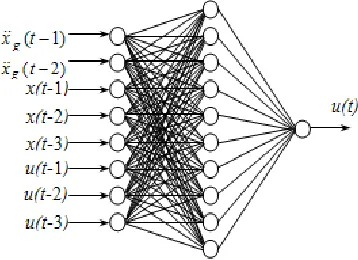
5.2. Network Architecture
In order to implement the control method described above,
we have used a three-layered feedforward neural network consisting of 8 inputs, 10 hidden units and 1 output. Figure 4 shows the architecture of the neural network.
Figure 4. Neural network architecture.
The input units represent the ground acceleration at two past time steps, the relative displacement at three past time steps and the control signal at three past time steps. The output unit represents the control to be sent to the actuator. The number of past time steps for each variable included in the input layer is chosen so as to provide the neural network with sufficient amount of information to implement the GMV control law and to take into consideration environ-mental changes. This choice is generally based on intuition and trial and error [6]. There are no systematic methods for determining these numbers.
5.3. Generation of Training Data
The set of training data is generated from the GMV con-trol of the structural system. The Kanai-Tajimi excitation model is used in the derivation of ARMAX model of the structure and the Kanai-Tajimi ground acceleration is used as an excitation in the base of the structure. 150 examples were selected from the 30 s control time history to train the network with Backpropagation algorithm.
We deduce that the training has been done on one sto-chatic model C. Any change of the stochastic model affect directly the regulator parameter for the classical algorithm.
6. Mathematical Model of Earthquake
Ground Motion
The earthquake ground acceleration is modeled as a un-iformly modulated non-stationary random process [10,22]
( ) ( ) ( )
t tx t xɺg ɺɺsɺ =ψ
(17)
where ψ(t) is a deterministic nonnegative envelope func-tion and xɺɺs
( )
t is a stationary random process with zero( ) 2 0 2 2 2 2 2 2 4 1 4 1 S g g g g g g + − + = ωω ξ ωω ωω ξ ω
φ (18)
Where: ξg,ωg are filter parameters and S0 is the constant spectral density of the white noise.
However, it can be shown that the velocity and dis-placement spectra, which are derived from the acceleration spectra that are described by equation (17), have strong singularities at zero frequency. These singularities can be removed by using high-pass filter, as suggested by Clough-Penzien [10]. Using such a second high pass filter, the Kanai-Tajimi spectrum is modified as follows to obtain the Clough-Penzien spectrum
( ) 2
0 2 2 2 2 4 2 2 2 2 2 2 4 1 4 1 4 1 S c c c c g g g g g c + − + − + = ωω ξ ωω ωω ω ω ξ ω ω ωω ξ ω
φ (19)
A particular envelope function ψ(t) given in the following will be used
( )
(
)
[
]
≥ − − ≤ ≤ ≤ ≤ < = 2 2 2 1 1 2 1 for exp for 1 0 for 0 for 0 t t t t a t t t t t t t t tψ (20)
where t1, t2 and a are parameters that should be selected appropriately to reflect the shape and duration of the earth-quake ground acceleration.
Numerical values of parameters are [15]:
t1=3s, t2=13s, a=0.26, ξg=0.65, ωg=19rad/s, ξc=0.6,
ωc=2rad/s, S0=0.8 10-2m/s.
The Kanai-Tajimi and Clough-Penzien ground accelera-tions have been simulated for yhe excitation of the structure. According to the parameter of this model we can determine the discrete model. So we obtain one valid regulator for the chosen structure.
But using neural network algorithm, we can obtain an in-finite kind of stochatic regulators from the ANN generali-zation.
7. Simulation Results
In order to demonstrate the efficiency of the neural net-work-based controller and show its superiority in compari-son with the GMV controller, a single-degree-of-freedom structure with the following structural properties [20] m=2921Kg, k=1389kN/m, ξ=0.0124 is used. An active tendon controller is installed in the story unit and the angle
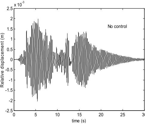
of incline of the tendons with respect to the floor is 25o. Thus, the control force vector from the controller is u/cos25o. Thus we can suppose that the force is applied at the top of the structure and assumed to be activated externally by an independent power supply. Figure 5 shows the open re-sponse for the seismic excitation.
Figure 5. Open loop response for ground accelerations.
To implement the GMV algorithm we have used a sam-pling period Ts=0.02s. Ponderation polynomials used in the GMV algorithm are:
PD(q-1)=1, PN(q-1) = 1 - 0.5q-1, Q(q-1)= 10-8
We have used to train the neural network a learning rate η of 0.2 for the first layer and 0.1 for the second layer. Weights were arbitrary initialized between –0.5 and 0.5. Training took around 2500 cycles to achieve an acceptable error.
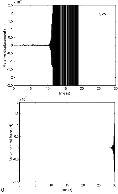
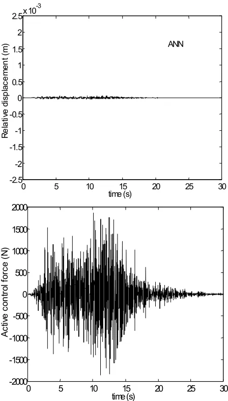
The building was subjected to excitations of Kanai-Tajimi model and a parameter variation (diminution of the struc-tural mass m of 20% at t=10s) for purposes of comparison. Figures 6 and 7 show the structural response for seismic escitation amplitude of 200%. Whereas in figure 8, we show that the classical algorithm can not maintain its perfor-mances. But in figure 9 we see the robustness of the pro-posed algorithm and the response is stable with the same calculated nework without any changes. Table I gives the output variance for each case.
Table 1 Output variance for different cases.
Kanai-Tajimi model
200% of
Ka-nai-Tajimi Diminution of m No control 3,4016.10-7 1,3606.10-6 2,5232.10-7
GMV 1,6286.10-10 6,5143.10-10 Divergence
ANN 1.7129.10-10 7.0974.10-10 1.7705.10-11
0 5 10 15 20 25 30
-2.5 -2 -1.5 -1 -0.5 0 0.5 1 1.5 2 2.5x 10
Figure 6. Classical GMV Structural response to 200% of Kanai-Tajimi ground acceleration.
0 5 10 15 20 25 30 -4
-3 -2 -1 0 1 2 3 4
x 10-3
time (s)
R
e
la
ti
ve
d
is
p
la
c
e
m
e
n
t
(m
) ANN
0 5 10 15 20 25 30
-4000 -3000 -2000 -1000 0 1000 2000 3000 4000
time (s)
A
c
ti
ve
c
o
n
tr
o
l
fo
rc
e
(
N
)
Figure 7. NN GMV approach Structural response to 200% of Kanai-Tajimi ground acceleration
0
Figure 8. Classical GMV Structural response to Kanai-Tajimi ground acceleration with structural parameter variation.
0 5 10 15 20 25 30
-4 -3 -2 -1 0 1 2 3 4
x 10-3
time (s)
R
e
la
ti
v
e
d
is
p
la
c
e
m
e
n
t
(m
)
GMV
0 5 10 15 20 25 30
-4000 -3000 -2000 -1000 0 1000 2000 3000 4000
time (s)
A
c
ti
v
e
c
o
n
tr
o
l
fo
rc
e
(
N
)
0 5 10 15 20 25 30
-2.5 -2 -1.5 -1 -0.5 0 0.5 1 1.5 2 2.5x 10
-3
time (s)
R
e
la
ti
v
e
d
is
p
la
c
e
m
e
n
t
(m
)
GMV
0 5 10 15 20 25 30
-1.5 -1 -0.5 0 0.5 1 1.5
2x 10
37
time (s)
A
c
ti
v
e
c
o
n
tr
o
l
fo
rc
e
(
N
0 5 10 15 20 25 30 -2.5
-2 -1.5 -1 -0.5 0 0.5 1 1.5 2 2.5x 10
-3
time (s)
R
e
la
ti
ve
d
is
p
la
c
e
m
e
n
t
(m
) ANN
0 5 10 15 20 25 30
-2000 -1500 -1000 -500 0 500 1000 1500 2000
time (s)
A
c
tiv
e
c
o
n
tr
o
l
fo
rc
e
(
N
)
Figure 9. ANN GMV Structural response to Kanai-Tajimi ground accele-ration with structural parameter variation.
It is easily seen that the neural controller has good per-formances comparable to those of the GMV controller. The neural controller was able to reduce the structural response with only a limited amount of control effort. But the im-portant result here is that the neural controller could com-pensate for structural parameter variation whereas the GMV controller performances are severely degraded and the control showed to be instable in this case. This result shows the robustness of the proposed algorithm against this kind of variations.
8. Conclusions
A neural network-based controller was used in this paper to overcome limitations of the classical GMV algorithm. Also to ovoid the use of adaptive algorithm which needs more stability analysis and more time calculation. Despite that the neural network was trained on a specified data including only the Kanai-Tajimi earthquake excitation model, it was able to generalize to non trained data and showed to have good performances with another types of
seismic excitation models. It has been shown also that the neural controller uses its generalization capabilities to compensate for structural parameter variation and maintains its good performances along all the control time history, whereas the GMV control performances become very bad since structural parameter variation will modify the AR-MAX model of the structure.
As a result, we can say that the neural network acquired control skills from the GMV controller, while using its intrinsic capabilities to positively interact with the envi-ronmental changes. We obtain a robust neural network GMV algorithm witch give much better result than the classical one. The aim was to present a simple robust algorithm based on the stochastic control theory for many kind of seismic excitations. According to the seismic excitation amplitude, it is possible to develop many controller for each excitation and then to choose the corresponding one. The calculation of one ANN controller is sufficient to maintain the perfor-mance of the closed system without any other calculation or using adaptive control theory. In our case we can calculate the ANN parameter once and then to implement this one in parallel calculators as transputer or equivalent circuits. These kind of solution is more convenient in seismic ap-plication for civil engineering.
References
[1] K. J. Åström, “Introduction to stochastic control theory”, Academic Press, 1970.
[2] K. J. Åström, “theory and applications of self tuning regu-lators”, Automatica, 13(99), 457-476.
[3] Pergamon press, (1977).K. J. Åström, “Computer-controlled systems”, Prentice-Hall, Inc., 1990.
[4] M.M. Al Imam and M. M. Mustapha,Robust minimum variance controller using over parametrized controller; ARPN Journal of Engineering and applied Sciences, vol 4; NO 10,pp11-18 December 2009.
[5] M.M. Al Imam and M. M. Mustapha, A Robust Controller for output variance reduction and minimum with application on permanent Field DC Motor; world Academy of science and technology, pp703-708, December 2009.
[6] K. Bani-Hani and J. Ghaboussi, “Nonlinear structural control using neural networks”, J. eng. mech., ASCE 124(3), 319-327 (1998).
[7] A. G. Chassiakos and S. F. Masri, “Modelling unknown structural systems through the use of neural networks”, Earthquake eng. struct. Dyn. 25, 117-128, (1996).
[8] D. W. Clarke, “Introduction to self tuning controller”, IEE, Control Eng. Series 15, H. Nichelson and B. H. Swanick, “self tuning and adaptive control : theory and application”, Peter pregrinus, 1981.
[9] D. W. Clarke, “Self tuning control of non-minimum phase systems”, Automatica 20(5), 501-517, (1984).
[11] J. P. Conte, A. J. Durrani and R. O. Shelton, “Response emulation of multistory buildings using neural networks”, Proc. First World Conf. Struct. Control, WP1, 59-68, (1994).
[12] P. J. Gawthrop, “Some interpretations of self tuning control-ler”, Proc. IEE 124(10), 889-894, (1977).
[13] J. Ghaboussi and A. Joghatie, “Active control of structures using neural networks”, J. eng. mech., ASCE 121(4), 555-567, (1995).
[14] L. Guenfaf, N. Bali, R. Illoul and M. S. Boucherit, “Perfor-mances study of multirate generalized minimum variance algorithm applied to robotic manipulators”, ITHURS’96, International conference, ENG’95 with IEEE.
[15] L.Guenfaf, “On the use of automatic control and neural networks in structural dynamics,” Phd Thesis, 2001, LCP, ENP, Algiers, Algeria.
[16] L.Guenfaf and Al, “Generalized minimum variance control for buildings under seismic ground motion”, Earthquake Eng. Strut. Dyn., Vol 30, Issue 7, pp945-960, 2001.
[17] M.J. Grimble Non-linear generalized minimum variance feedback, feedforward and tracking control Automatica 41 (2005) pp 957 – 969 Elsevier.
[18] G. W. Housner and Al, “Structural control: past, present and future”, J. eng. mech., Special issue ASCE 123(9), 897-970, (1997).
[19] A. Patetea, K. Furuta, M. Tomizuka Self-tuning control based on generalized minimum variance criterion for au-to-regressive models Automatica 44 (2008) pp1970–1975.
[20] H. A. Smith, W. -H. Wu and R. I. Borja, “Structural control considering soil-structure interaction effects’” Earthquake eng. struct. Dyn. 23, 609-626, (1994).
[21] P. Venini and Y.-K. Wen, “Hybrid vibration control of MDOF hysteretic structures with neural networks”, Proc. First World Conf. Struct. Control, TA3, 53-6, (1994).
[22] J. N. Yang, A. Akbapour and P. ghaemmaghami, “New optimal control algorithms for structural control”, J. eng. mech. ASCE 113(9), 1369-1386, (1987).