Multi Criteria Decision Making Technique For Machine Learning Algorithms: Iterative And Non-Iterative Algorithms

2392

Multi Criteria Decision Making Technique For

Machine Learning Algorithms: Iterative And

Non-Iterative Algorithms

Abstract: With increasing amount of data generated every day, there is a need to extract useful information from the data which is an important problem

to be solved. Machine learning is a method that enables the computer system to have the intelligence by analyzing the data and building an automated analytical model. The algorithms in machine learning are broadly classified as either iterative or non-iterative algorithms. An optimization algorithm plays a key role in machine learning that is solved by iterative methods that are executed iteratively to generate optimum solution or till a satisfactory solution is obtained. A non-iterative algorithm is computationally faster than iterative algorithms as it does not require iteration or little iter ation to train the data. This paper makes an analysis of these iterative and non-iterative algorithms and performs comparison upon their respective advantages and drawbacks. These algorithms are compared based on various parameters such as time taken to bu ild the model, correctly and wrongly classified instances, mean absolute error, root means square error, true positive, false positive, precision and recall are computed. Multi Criteria Decision Making method such as TOPSIS is used to improve the efficiency of the decision making process by suggesting best machine learning technique that improves classification

Index Terms: Iterative, supervised, unsupervised, machine learning, data mining, Multi Criteria Decision Making

——————————  ——————————

I.

INTRODUCTION

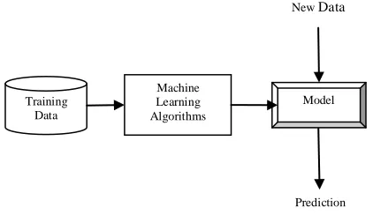
Machine learning algorithm [1-24] uses computers system that could automatically learn from past observations and find predictive models to make accurate predictions on future data. The main goal of machine learning algorithm is to make highly accurate prediction on the supplied data. It is difficult to make all decisions with the input data that is supplied and hence algorithms develop knowledge from past experience. Figure 1 shows the overview of machine learning algorithms. The training data is fed as input to the machine learning algorithms that are used to discover predictive relationships. As a result of the training the dataset a model is built. Using the model generated future data (test data) can be predicted. The algorithms that are widely adopted in machine learning are supervised learning and unsupervised learning that are classified as either iterative or non-iterative based on their way of execution. Semi-supervised and reinforcement learning are other machine learning algorithms that are rarely used. Supervised learning [25-30] is a machine learning method that maps input and output based on the labeled training data which can be used to predict the future data. The goal of supervised machine learning is to build a model and when exposed to new data, the performance of the machine must be improved. Let us consider an example for predicting whether there will be a patient with cancer or not. You have set of data on previous patient‘s history including name, age, address, height, weight, pressure etc. you can compare this with the previous cancer patients. The existing data can be combined together to form a model to predict whether the new patient will have cancer or not. A Supervised learning algorithm is categorized as classification (if the output is discrete) and regression (if the output is continuous). Classification is a method of predicting the category or class the new observation belongs to based on the training data whose category is already known. Classification problem predicts whether the patient will have cancer, with possible class labels as yes or no. On the other hand, regression predicts the relationship among observation of continuous measurement.

Regression is used widely in weather forecasting and stock market prediction.

Figure 1: Overview of Machine Learning algorithms

An unsupervised learning is a machine learning method where unlabeled dataset is given to the system and it must find the relationship within data. The goal of unsupervised learning is to group the data together and identify the existing patterns in the data. An example to unsupervised learning is to group customers based on their purchase pattern as big brand shopper, seasonal spender, value conscious shopper etc. Semi- supervised learning [31-42] is another machine learning method that uses both labeled and unlabeled data for training. The algorithm works well when there is few labeled data and large number of unlabeled data. An example for semi-supervised learning includes ATM fraud identification by looking the persons face on the security camera. Reinforcement learning [43-55] is also a machine learning method in which the algorithm discovers the pattern or the relationship within the data through trial and error method. There are three main components involved which include an agent who makes decision, environment where the agent interacts and the action that the agent must perform. The goal of this algorithm is to identify best policy from the past experience to make accurate decisions. Reinforcement learning is used in robotics in which the sensor readings are continuously

Prediction Training

Data

Machine Learning Algorithms

2393

recorded and the algorithm determines the next action to be performed.

II.

MACHINE LEARNING ALGORITHMS:

Machine learning algorithm predicts a model based on the interaction with past experience to predict the future data. Figure 2 shows the categorization of machine learning algorithms. Machine learning algorithms are broadly classified as supervised and unsupervised that are categorised as either iterative or non-iterative which are discussed in detail in the following sections.

Figure 2: Categorization of Machine Learning algorithms

III.

ITERATIVE ALGORITHMS

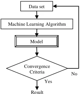
Machine learning is a mechanism of building an analytical model to perform data analysis. Machine learning algorithms iteratively learn from the data that allows the machine to find the hidden patterns within the data. The goal of iterative algorithm is to find the optimum solution from the data set. These algorithms learn from previous experience that is reliable and the repeatable decisions are taken to obtain optimum solution. Most of the algorithms in machine learning are iterative which usually takes some iteration to achieve a satisfactory result. A threshold (stopping criteria) can be set to the number of iterations as future iteration may result in minor changes to the data. The algorithm iteratively increases the accuracy of the prediction and proceeds until the convergence criteria (stopping criteria) or when the difference between the successive iteration values becomes small. Figure 3 shows the overview of iterative algorithm where the dataset is loaded and machine learning algorithm is applied to it and the model is generated. The process is iterated till the stopping criterion is satisfied. In the following section we will discuss the iterative models in detail.

A. Iterative supervised algorithms

Iterative supervised learning method learns from the data collect in the past to construct a model and is repeated iteratively till the convergence criterion is met. In this section we discuss in detail about the various iterative supervised learning algorithm such as decision trees, random forests, support vector machines, etc.

Figure 3: Overview of Iterative Algorithm

1. Decision Tree

Decision tree [56-62] is a predictive learning method that performs classification that can be represented and modeled as a tree. The goal of this algorithm is to construct a model which could predict the value of the new data by learning decision rules from the actual values of attributed in the data.

Figure 4: Decision tree constructed using Weka tool for the weather dataset.

Figure 4 shows the decision tree constructed using weka tool that contains decision nodes and leaf nodes. Decision nodes or internal nodes specifies test on the attribute whereas leaf nodes specifies the class. The tree is traversed from top-to-bottom based on the attribute values for a new instance (test instance) till the leaf node is reached. The decision tree is learned by splitting the dataset into subsets based attribute value test that is repeated in a recursive manner and continues till all the instance belongs to same class. In each recursion the best attribute is chosen in such a way impurity is minimized. An important aspect of decision making is the choice the impurity function and information gain and information gain ratio are two popular methods. Information gain is based on entropy and information theory whereas gain ratio is calculated based on the gain obtained by entropy with respect to the attribute values. Decision tree has lot of benefits like it is easy to understand, handles continuous and discrete values, reliable, robust and works well for large datasets. It includes algorithms like ID3, C4.5 etc.

2. Random Forest:

Random forest [66-70] or random decision forest is an ensemble of decision tree. The collection of these decision

Data set

Machine Learning Algorithm Model

Result Yes

No Convergence

Criteria Machine

Learning Algorithms

Iterative Algorithms

Non-Iterative Algorithms

Supervised Algorithms

Supervised Algorithms

Unsupervised Algorithms Unsupervised

2394

trees are executed iteratively to form the forest. It is a flexible machine learning algorithm that works for classification and regression. To carry out the classification for an attribute, each tree in the forest provides a classification and the tree can vote for the class. The forest will choose the classification that has the maximum votes. In case of regression problems, the trees are grouped to produces numerical response value from which the predictor set is chosen randomly. It can handle missing values and outliers in an efficient way. It uses out of bag samples that takes one third data for test and estimates error which is known as out of bag error.

Figure 5: Tree generated by random forest algorithm using rapid miner for golf testset dataset

Figure 5 shows the plot of two of the trees generated random forest algorithm using rapid miner tool [71] for a

sample dataset available in it.

3. Support Vector Machine:

A support vector machine (SVM) [72-83] is a supervised learning method that works well for classification and regression problems. The data item in this algorithm is plotted in n-dimensional space in which each coordinate corresponds to a feature. The hyper-plane also called as decision boundary or decision surface is constructed to differentiate the class in the plot and predict the category in which it belongs. The hyper-plane separates the n-dimensional space into two portions and is called as line in 2d space and plane in 3d space. A good hyper-plane can be achieved if it has largest distance to the nearest data point. SVM is most suitable for classification problem and provides high accuracy in case of high dimensional data.

Figure 6: SVM with different cases: linear seperable (left), linear seperable (middle) and linear

non-separable (right)

Figure 6 shows an SVM with different cases like linear separable SVM, linear seperable SVM and linear non-separable SVM. In linear non-separable SVM there is a linear line that separates the two classes and it uses mapping function that converts data in input space to data in feature space. In many real life datasets the decision boundaries are nonlinear and it is handled in the same way as in case

of linear seperable where the input data from in original space is transformed into another space (also called as feature space) where the decision boundary can separate the classes. In practical situation there may be noisy data and it is difficult to separate the data points in n-dimensional space and the instances may be labelled incorrectly. The method uses soft margin SVM and Lagrange multipliers to perform the classification by changing the labels of the instances iteratively to attain accuracy in SVM. There is algorithm called iterative SVM (I-SVM) one of the partially supervised method in which a classifier is constructed for iteration and the algorithm is repeated till no document is classified as negative.

B. Iterative unsupervised algorithms

Iterative unsupervised learning method consists of unlabeled dataset and it is the responsibility of the machine to identify the relationship that exists in the data by executing it iteratively till the convergence criterion is met. In this section we discuss in detail about the various iterative unsupervised learning algorithm such as k- means clustering, expectation maximization, self-organizing maps, etc.

1. K-means

K-means [84-95] is an unsupervised learning algorithm and also a widely used partitional clustering algorithm. The algorithm iteratively clusters the data set based on the value of K that the user specifies. It uses distance function to cluster the data points. For every cluster, centroid (cluster center) is assigned which is calculated by considering the mean of the data points present in the cluster and hence the algorithm is called as K-means algorithm.

Figure 7: Overview of K-means algorithm

Figure 7 shows the overview of K-means clustering algorithm. Initially the algorithm randomly considers K data points in the cluster as seed points. The distance function is calculated between the seed and every data point. The data point is assigned to the centroid that is close to it and hence all the data points and the centroid together form a cluster. The process is repeated again and again till the stopping criterion is met. The algorithm could be stopped when one of the following conditions is encountered: no change in

Number of Clusters K chosen Initial centroid assigned for each

cluster

Stop

No - Iterate Distance function calculated

Centroid reassigned

Yes Stopping

2395

cluster center, data points do not change from one cluster to another and the sum of square error is minimum. Data points that lie within the cluster are similar and they are dissimilar outside the cluster. The algorithm is efficient, faster and works well for data sets that are distinct.

2. Expectation maximization

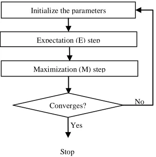
Expectation maximization (EM) [96-102] is an iterative algorithm that estimates maximum likelihood for unobserved variables. The algorithm is carried out in two steps. Expectation (E) step is the first step that fills missing values based on parameter estimated. Maximization (E) step is the other step that re-computes the parameters and maximizes the likelihood. The algorithm works iteratively till there the parameter converges.

Figure 8: Overview of Expectation Maximization

Figure 8 shows the overview of Expectation Maximization where the parameters are initialized followed by Expectation (E) and Maximization (M) steps that are iterated till the parameter converges.

3. Self organizing maps

Kohonen developed self organizing maps (SOM) [103-108] which is an unsupervised learning method. The main idea of this method is to identify the structure present in the data and reduce the dimensionality of the data using self organizing neural networks. SOM uses competitive learning for clustering the data, where input patterns are clusters in discrete clusters. In order to preserve the neighborhood information topological maps are constructed. The learning process of SOM is carried out without any supervision. It works by two steps: training and mapping. The input is sent to the network and the output that is obtained is compared with the target. If there is a difference in the output, the weights are adjusted and the process is repeated iteratively. Figure 9 shows the working of self organizing maps.

IV.

NON - ITERATIVE ALGORITHMS

Non-iterative learning method learns from the data collect in the past to construct a model that is executed immediately without any iteration. In this section we discuss in detail about the various non-iterative learning algorithms such as naive bayes, k-nearest neighbor, linear regression and case based reasoning etc.

Figure 9: Overview of Self-organizing maps

1. Naive Bayes

Naive bayes [109-116] is a classification technique that applies bayes theorem by an assumption that the pair of features is independent. It is easy to construct and can easily predict the class in which the test data belongs. It works well for large data set. The classification in this algorithm is carried out by estimating the posterior probability and the class with highest probability is assigned to the test sample. The probability to construct a naive bayesian classifier can be built in a single iteration and the algorithm is extremely efficient. Most naive bayesian algorithm handles discrete attributes, but real world data sets can be of any type (discrete/continuous). Therefore in order to work with naive Bayesian classifier the dataset should be converted to discrete attributes before further processing. The algorithm has a zero count problem where the attribute in the test set may not appear in the training set and results in a 0 probability that wipes out other probability. To overcome this problems small sample correlation can be added into the probability or smoothing techniques can be used. Missing values are ignored in this algorithm.

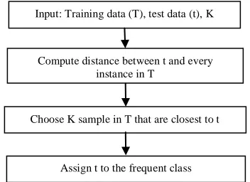
2. K-Nearest Neighbor

K-nearest neighbor [117-125] is supervised learning method that works for both classification and regression. It is lazy learning [126-130] method in which it learns only when a new data needs to be classified. It records all different cases and classifies new data based on the majority vote of their k-neighbors. It uses distance function to measure the k-nearest neighbors and assigns the class that is closest. Assigning the value of k is one important challenge in this algorithm. The number of nearest neighbor is determined based on validation set or cross validation set on the training data. The algorithm is strong, accurate and works for arbitrary shaped boundaries. Figure 10 shows the flow chart of K-nearest neighbor algorithm.

Randomize weights

Grab Input vector

Stop Yes

No Converges?

Traverse each node

Adjust weight

Initialize the parameters

Expectation (E) step

Stop Yes

No Converges?

2396 Figure 10: Flow chart of K-nearest neighbor algorithm

3. Linear Regression

Linear regression [131-135] is a supervised learning method that finds the relation between any two variables. The observed data is fit into the linear equation. Based on one variable, the other variable can be found and the variable that we are going to predict is called as criterion variable. The variable based on which our prediction is carried out is called as predictor variable. Linear regression also called as simple regression which plots a straight line when the criterion variable is the function of predictor variable. It finds the best fitting line called as regression line which is chosen based on the factor that minimizes sum of square error. This is a statistical tool that works well for finding relationship between two continuous variables.

Figure 11: Linear regression

Figure 11 shows linear regression where X denotes criterion variable and Y denotes predictor variable. This algorithm is interpretable and requires minimal tuning. The algorithm works fast and is a non-iterative method. Linear regression can be used to predict the future sales of the company based on the monthly sales of the company.

D. Case Based Reasoning

Case based reasoning (CBR) [136-141] is a supervised learning method which solves a new problem based on the previous problem. In this method, a new example is predicted based on the similar cases that are close to it. This algorithm does not require previous processing and can be predicted during query time. It works well for classification and regression problems. The algorithm works well for complicated cases and to similarity distance measures are used. It has 4 phases: retrieve, reuse, revise and retain. When a new case is presented, similar case must be retrieved and reuse the retrieved case for the new problem. Evaluate and revise the cases. Conclude whether to retain this case or not. Example to this algorithm is when a customer goes to mobile service center; the service man

handles this problem by comparing it with the previous cases that were already faced.

V.

TECHNIQUE FOR ORDER PREFERENCE

BY SIMILARITY TO THE IDEAL SOLUTION

(TOPSIS)

TOPSIS[142-151] is a multi-criteria decision analysis method that ranks the alternative based on the distance to positive ideal solution and the distance to negative ideal alternative. Positive ideal solution is the best value obtained for all the considered criteria and Negative ideal solution is the worst value for all the considered criteria. If we have ‗m‘ alternatives and ‗n‘ criteria then xij denotes the performance value of ith alternative for jth criterion. Let J represent the set of benefit criteria and J' represent the set of negative criteria. The steps involved in TOPSIS method are as follows:1. Construction of normalized matrix. This method transforms the criteria of alternatives into normalized form. This method is chosen, as the performance values of alternatives for different criteria will have conflicting dimensions. Normalization can be carried out in two different ways: Linear normalization and Vector normalization. The vector method of normalization is given as follows:

(1)

2. Construction of weight vector

Based on the objective decide the relative importance (i.e.,weights) of different criteria. A set of weights wj is framed (for j=1, 2,.., n) such that

(2)

3. Construction of weighted normalized decision matrix.

This step involves the construction of weight vector for each criteria and it is denoted as wj . Then multiply each column of the normalized decision matrix by its associated weight. Weighted normalized decision matrix is calculated as follows:

(3)

4. Determination of the positive ideal and negative ideal solutions.

Positive ideal solution and negative ideal solution can be determined with the help of the following equations.

Positive ideal solution:

(4)

(5)

Negative ideal solution:

(6)

(7)

5. Calculation of the separation measure for each alternative.

This step calculates the separation measure of an alternative from positive ideal solution and also from negative ideal solution.

Input: Training data (T), test data (t), K

Compute distance between t and every instance in T

Choose K sample in T that are closest to t

2397

Separation measure from positive ideal solution is calculated as follows:

(8) Separation measure from negative ideal solution is calculated as follows:

(9)

6. Calculation of the relative closeness coefficient of each alternative.

This step calculates the similarity of the alternatives by considering positive ideal solution and negative ideal solution. Relative closeness coefficient value is calculated as follows:

(10)

Select the alternative with high relative closeness coefficient value.

VI.

PERFORMANCE COMPARISON OF

ITERATIVE AND NON-ITERATIVE

ALGORITHMS USING TOPSIS

The algorithms that discussed above (iterative and non-iterative) have been tested in weka for the weather nominal dataset. Table 1 and Table 2 show the comparison of various machine learning algorithms in weather and UCI dataset respectively. Here, the machine learning algorithms are alternatives; TOPSIS selects the best algorithm based on the criteria including execution time, correct classification, wrong classification, Mean absolute error, root mean squared error, precision and recall. Here classification accuracy is the benefit criteria and other two are cost criteria. If we assign the weight values for the criteria as w1=0.01(execution time), w2=0.3(correct classification), w3=0.2(wrong classification), w4=0.01 (Mean absolute error), w5=0.01 (root mean squared error), w6=0.01 (precision), w7=0.01 (recall), then the results of TOPSIS for chosen weight factor is given in the table 3. From this TOPSIS method, we can conclude that iterative algorithms are the best techniques for classification. The comparison of iterative and non iterative algorithms was done on large data like telescope data with 19,020 instances [11 attributes] and letter recognition data with 20,000[17 attributes] instances taken from UCI machine learning repository were tested as 10 cross validation folds on the data. The result analysis is shown in Table 2. Performance Analysis of the iterative and non iterative methods on telescope data is given in the Figure 12. Similarly time complexity was measured in Letter Recognition Data as given in the Figure 13.

Figure 12: Time Complexity Analysis on Telescope Data

Figure 13: Time Complexity Analysis on Letter Recognition Data

The iterative unsupervised algorithms were then applied on large data of telescope and letter recognition. The results proved that based depending on number of iterations and clusters to converge the time for execution increases whereas it provides good results on clustering with less mean squared error. Figure 14 shows the result Time Complexity Analysis on Iterative unsupervised methods.

Figure 14: Time Complexity Analysis on Iterative unsupervised methods

Ti

m

e

(s

e

c

o

n

d

s)

Ti

m

e

(s

e

c

o

n

d

s)

Ti

m

e

(s

e

c

o

n

d

2398 TABLE I. PERFORMANCE COMPARISON OF ITERATIVE AND NON-ITERATIVE ALGORITHM – WEATHER DATASET

Machine Learning Method Al g o ri th m T im e t a k e n t o b u ild t h e m o d e l C o rre c tl y c la s s if ie d in s ta n c e s In c o rr e c tl y c la s s if ie s in s ta n c e s M e a n a b s o lu te e rro r R o o t m e a n s q u a re d e rr o r T P ra te F P ra te Pre c is io n R e c a ll Iterative

Decision tree 0.01 sec 85.71 % 14.28% 0.1429 0.378 0.85 0.16 0.85 0.85 Random forest 0.03 sec 71.42% 28.57% 0.3462 0.4227 0.71 0.33 0.71 0.71 SVM 0.14 sec 64.28% 35.71% 0.3571 0.5976 0.

64 0.46 0.62 0364

Non- Iterative

Naïve bayes 0 sec 57.14% 42.85% 0.4374 0.4916 0.57 0.59 0.52 0.57 KNN 0 sec 57.14% 42.85% 0.4911 0.5985 0.57 0.51 0.57 0.57 Linear

Regression 0 sec - - 0.4978 0.5972 - - - -

TABLE II. PERFORMANCE COMPARISON OF ITERATIVE AND NON-ITERATIVE ALGORITHM LARGE UCI DATASET

Data Machine Learning Method Al g o ri th m T im e t a k e n t o b u ild t h e m o d e l C o rre c tl y c la s s if ie d in s ta n c e s In c o rr e c tl y c la s s if ie s in s ta n c e s M e a n a b s o lu te e rr o r R o o t m e a n s q u a re d e rr o r T P ra te F P ra te Pr e c is io n R e c a ll Telescop e Iterative

Decision tree 3.78 85.06% 14.95% 0.1955 0.3509 0.851 0.211 0.849 0.851 Random

forest 10.48 87.32% 12.68% 0.1968 0.307 0.943 0.255 0.872 0.906 SVM 5.14 79.15% 20.85% 0.2085 0.4566 0.792 0.297 0.788 0.792 Non-

Iterative

Naive bayes 0.03 72.69% 27.31% 0.2789 0.4859 0.727 0.433 0.723 0.727 KNN 0.04 81.35% 18.65% 0.1965 0.3847 0.814 0.307 0.823 0.814 Linear

Regression 0.02 - - 0.3591 0.4238 - - - -

Letter Recogniti on

Iterative

Decision tree 1.58 87.92% 12.08% 0.0106 0.0907 0.879 0.0005 0.879 0.879 Random

forest 8.52 96.37% 3.63% 0.0131 0.0622 0.964 0.001 0.964 0.964 SVM 8.08 82.44% 17.56% 0.0711 0.1861 0.824 0.007 0.831 0.824 Non-

Iterative

Naïve bayes 0.05 64.01% 35.99% 0.0323 0.1391 0.640 0.014 0.655 0.640 KNN 0.10 94.58% 5.42% 0.0145 0.0708 0.946 0.0002 0.947 0.946 Linear

2399 TABLE III. PERFORMANCE COMPARISON OF ITERATIVE AND NON

-ITERATIVE ALGORITHM USING TOPSIS

Classification Algorithm Relative closeness coefficient Rank

Decision Tree 0.992314 1

Random Forest 0.523662 2

Support Vector Machine 0.370669 3

Naive Bayes 0.205737 4

KNN 0.205736 5

Linear Regression 0.082748 6

VII.

CONCLUSION

Thus the machine learning algorithms that are iterative and non-iterative are compared and the best algorithm is decided using Multi Criteria Decision Making (MCDM) technique like TOPSIS. Iterative algorithm that are supervised are discussed that includes decision tree, random forest and support vector machines. Iterative unsupervised methods like self organizing maps, expectation maximization and k-means are discussed. Finally non-iterative algorithms like naive bayes, k-nearest neighbor, linear regression and case based reasoning algorithms are analyzed. These algorithms are compared based on various parameters such as time taken to build the model, correctly and wrongly classified instances, mean absolute error, root means square error, true positive, false positive, precision and recall are computed for given dataset. It was analyzed that non-iterative algorithms executed fast when compared with iterative algorithms whereas the accuracy was high in case of iterative algorithm. Thus MCDM detects the best technique among different machine learning techniques for classification.

VIII.

REFERENCES

[1] Atul Kumar, Sameep Mehta, and Deepak

Vijaykeerthy,2017. An Introduction to Adversarial Machine Learning. In P. Krishna Reddy, AshishSureka, Sharma Chakravarthy, and SubhashBhalla, editors, Big Data Analytics, pages 293–299, Cham, Springer International Publishing.

[2] AngluinD, 1988Queries and Concept Learning. In Machine Learning, pages 319–342. Springer.

[3] TommasoDreossi, AlexandreDonz´e, and Sanjit A Seshia, 2017 ,Compositional Falsification of Cyber-Physical Systems with Machine Learning Components. In NASA Formal Methods Symposium, pages 357–372. Springer.

[4] Javier Garc´ıa and Fernando Fern´andez, 2015. A Comprehensive Survey on Safe Reinforcement Learning. Journal of Machine Learning Research, 16:1437– 1480

[5] Eric Wong and J Zico Kolter,2017. Provable Defenses against Adversarial Examples via the Convex Outer Adversarial Polytope. arXiv preprint arXiv:1711.00851. [6] Fredrik Olsson, 2009 A literature survey of active

machine learning in the context of natural language processing. SICS Technical Report. 1 edition

[7] ErkanTuncali C,Fainekos G, Ito H, andKapinski J April 2018. Simulation based Adversarial Test Generation for

Autonomous Vehicles with Machine Learning

Components. ArXiv e-prints

[8] SiccoVerwer, Mathijs de Weerdt, and

CeesWitteveenMar 2012. Efficiently identifying

deterministic real-time automata from labeled data. Machine Learning, 86(3):295–333

[9] Qinglai Wei and Derong Liu 2015. Neural-network-based adaptive optimal tracking control scheme for discrete-time nonlinear systems with approximation errors.Neurocomputing, 149:106 – 115. Advances in neural networks Advances in Extreme Learning Machines.

[10] Witten I and Frank E 2000 Data Mining: Practical Machine Learning Tools and Techniques with Java Implementations. San Francisco: Morgan Kaufmann [11] Langley P 1996 ―Elements of machine learning‖,

Morgan Kaufmann Publishers

[12] MarslandS 2015 Machine learning: an algorithmic perspective. CRC press

[13] Buczak A L andGuven E, Oct. 2015 ―A survey of data mining and machine learning methods for cyber security intrusion detection,‖ IEEE Communications Surveys & Tutorials, vol. 18, no. 2, pp. 1153–1176 [14] Nguyen T T and Armitage G 4th Q 2008. ―A survey of

techniques for internet traffic classification using machine learning,‖ IEEE Communications Surveys & Tutorials, vol. 10, no. 4, pp. 56–76

[15] Bkassiny M, Li Y, and Jayaweera S K Oct. 2012 ―A survey on machine learning techniques in cognitive radios,‖ IEEE Communications Surveys & Tutorials, vol. 15, no. 3, pp. 1136–1159.

[16] M. Bkassiny, Y. Li, and S. K. Jayaweera, Oct. 2012 ―A survey on machinelearning techniques in cognitive radios,‖ IEEE Communications Surveys & Tutorials, vol. 15, no. 3, pp. 1136–1159.

[17] Murphy K P,2014 ―Machine learning, a probabilistic perspective,‖

[18] Zibar D, PielsM,Jones R, and Schaeffer C GMar. 2016.

―Machine Learning Techniques in Optical

Communication,‖ IEEE/OSA Journal of Lightwave Technology, vol. 34, no. 6, pp. 1442–1452,

[19] RottondiC,Barletta L, Giusti A, and Tornatore M Feb 2018., ―Machinelearning method for quality of transmission prediction of unestablishedlightpaths,‖ IEEE/OSA Journal of Optical Communications and Networking, vol. 10, no. 2, pp. A286–A297

[20] Thrane J, Wass J, PielsM,Diniz J C M, Jones R, and ZibarDFeb. 2017 ―Machine Learning Techniques for Optical Performance Monitoring From Directly Detected PDM-QAM Signals,‖ IEEE/OSA Journal of Lightwave Technology, vol. 35, no. 4, pp. 868–875.

[21] Peteiro-BarralD,Guijarro-BerdinasB, 2013"A survey of methods for distributed machine learning" in Progress in Artificial Intelligence, Springer, vol. 2, no. 1, pp. 1-11. [22] Berral-GarciaJ L 2016, "A quick view on current techniques and machine learning algorithms for big data analytics", 18th International Conf. on Transparent Optical Networks, pp. 1-4,.

[23] Qui J, Wu Q, Ding G, Xu Y, Feng S2016"A survey of machine learning for big data processing", EURASIP Journal on Advances in Signal Processing, vol. 2016, no. 67, pp. 1-16.

2400

[25] KotsiantisS B 2007, ―Supervised Machine Learning: A Review of Classification Techniques‖, Informatica, Vol. 31, No. 3, pp. 249-268.

[26] Pierre Geurts, AlexandreIrrthum, Louis Wehenkel 2009, ―Supervised learning with decision tree-based methods in computational and systems biology‖, Molecular BioSystems, Vol. 5, No. 12, pp. 1593-1605.

[27] Panigrahi P K2012, "A comparative study of supervised machine learning techniques for spam e-mail filtering", in Computational Intelligence and Communication Networks(CICN), vol. 4, pp. 506-512. [28] Chen X, Mériaux F, and ValentinSJun. 2013,

―Predicting a user‘s next cell with supervised learning based on channel states,‖ in Proc. IEEE 14th Workshop Signal Process. Adv. Wireless Commun. (SPAWC), Darmstadt, Germany , pp. 36–40.

[29] Batista, G., &Monard, M.C., An Analysis of Four Missing Data Treatment Methods for Supervised Learning, Applied Artificial Intelligence, vol. 17, pp.519-533.

[30] Basu, S., A. Banerjee, and R. Mooney2002, ―Semi-supervised clustering by seeding‖, in Proceedings of International Conference on Machine Learning (ICML-2002).

[31] Zhu, X., Rogers, T., Qian, R., &Kalish, C. 2007. Humans perform semi-supervised classification too. Twenty-Second AAAI Conference on Artificial Intelligence (AAAI-07).

[32] Zhu, X., Lafferty, J., &Ghahramani, Z. 2003c. Semi-supervised learning: From Gaussian fields to Gaussian

processes (Technical Report CMU-CS-03-175).

Carnegie Mellon University

[33] Zhu, X., Ghahramani, Z., & Lafferty, J. 2003a. Semi-supervised learning using Gaussian fields and harmonic functions. The 20th International Conference on Machine Learning (ICML).

[34] Yang, X., Fu, H., Zha, H., & Barlow, J. 2006. Semi-supervised nonlinear dimensionality reduction. ICML-06, 23nd International Conference on Machine Learning.

[35] Xu, L., &Schuurmans, D. 2005. Unsupervised and semi-supervised multi-class support vector machines. AAAI-05, The Twentieth National Conference on Artificial Intelligence.

[36] Weston, J., Leslie, C., Zhou, D., Elisseeff, A., & Noble, W. S.2004. Semi-supervised protein classification using cluster kernels. Advances in neural information processing systems. Cambridge, MA: MIT Press. [37] Tong, W., & Jin, R. 2007. Semi-supervised learning by

mixed label propagation. Proceedings of the Twenty-Second AAAI Conference on Artificial Intelligence (AAAI).

[38] Sindhwani, V., Niyogi, P., Belkin, M., &Keerthi, S. 2005c. Linear manifold regularization for large scale semi-supervised learning. Proc. of the 22nd ICML Workshop on Learning with Partially Classified Training Data.

[39] Rosenberg, C., Hebert, M., &Schneiderman, H. 2005. Semi-supervised self-training of object detection models. Seventh IEEE Workshop on Applications of Computer Vision.

[40] Oliveira, C. S., Cozman, F. G., & Cohen, I. 2005. Splitting the unsupervised and supervised components

of semi-supervised learning. Proc. of the 22nd ICML Workshop on Learning with Partially Classified Training Data. Bonn, Germany.

[41] Niu, Z.-Y., Ji, D.-H., & Tan, C.-L. 2005. Word sense disambiguation using label propagation based semi-supervised learning. Proceedings of the ACL.

[42] Richard S. Sutton and Andrew G. Barto1998, ―Reinforcement Learning: An Introduction‖, Cambridge, MA: MIT Press.

[43] Arulkumaran K, Deisenroth M P,Brundage M, and Bharath A AAugust 2017 A Brief Survey of Deep Reinforcement Learning. ArXiv e-prints.

[44] Aslund H, Mahdi El Mhamdi E, Guerraoui R, and Maurer AMay 2018. Virtuously Safe Reinforcement Learning. ArXiv e-prints.

[45] Felix Berkenkamp, MatteoTurchetta, Angela Schoellig, and Andreas Krause 2017. Safe Model-based Reinforcement Learning with Stability Guarantees. Advances in Neural Information Processing Systems 30, pages 908–918. Curran Associates, Inc.,

[46] Nathan Fulton and Andr´ePlatzerFebruary 2-7 2018. Safe Reinforcement Learning via Formal Methods: Toward Safe Control Through Proof and Learning. Proceedings of the ThirtySecond AAAI Conference on Artificial Intelligence, New Orleans, Louisiana, USA. AAAI Press.

[47] Javier Garc´ıa and Fernando Fern´andez2015. A Comprehensive Survey on Safe Reinforcement Learning. Journal of Machine Learning Research, 16:1437– 1480.

[48] Leslie Pack Kaelbling, Michael L. Littman, and Andrew W. Moore1996. Reinforcement Learning: A Survey. CoRR, cs.AI/9605103.

[49] RushikeshKamalapurkar, Joel A Rosenfeld, and

Warren E Dixon2016. Efficient model-based

reinforcement learning for approximate online optimal control.Automatica, 74:247–258.

[50] RushikeshKamalapurkar, Patrick Walters, Joel Rosenfeld, and Warren Dixon2018. Reinforcement Learning for Optimal Feedback Control: A Lyapunov-Based Approach. Springer.

[51] Qingkai Liang, FanyuQue, and EytanModiano2018. Accelerated PrimalDual Policy Optimization for Safe Reinforcement Learning. CoRR, abs/1802.06480. [52] RemiMunos, Tom Stepleton, Anna Harutyunyan, and

Marc G. Bellemare2016. Safe and Efficient Off-Policy Reinforcement Learning.CoRR, abs/1606.02647.

[53] ShashankPathak, Luca Pulina, and Armando

TacchellaApr 2018. Verification and repair of control policies for safe reinforcement learning. Applied Intelligence, 48(4):886–908.

[54] Kaelbling, L., Littman M, and Moore A1996, ―Reinforcement learning: A survey.Journal of Artificial Intelligence Research‖, p. 237–285.

[55] Hyafil, L. and R. Rivest 1976, ―Constructing optimal binary decision trees is NPcomplete‖, Information Processing Letters, 5(1): p. 15-17.

[56] JhaS,Raman V, and T.and Francis M. Pinto,

A.andSahai2017. On Learning Sparse Boolean

Formulae for Explaining AI Decisions. In NFM 2017: NASA Formal Methods, pages 99–114. Springer. [57] K. Karimi and Hamilton H J 2011, "Generation and

2401

International Journal of Computer Information Systems and Industrial Management Applications, Volume 3

[58] Alsabti K., Ranka S. and Singh VAugust

1998.,CLOUDS: A Decision Tree Classifier for Large Datasets, Conference on Knowledge Discovery and Data Mining (KDD-98). Attneave F., Applications of Inf [59] Buntine W., Niblett T1992., A Further Comparison of

Splitting Rules for DecisionTree Induction. Machine Learning, 8: 75-85.

[60] Esposito F., Malerba D. and Semeraro G1997.,A Comparative Analysis of Methods for Pruning Decision Trees. EEE Transactions on Pattern Analysis and Machine Intelligence, 19(5):476-492.

[61] Fayyad U., and Irani K. B.1992,The attribute selection problem in decision tree generation. In proceedings of Tenth National Conference on Artificial Intelligence, pp. 104–110, Cambridge, MA: AAAI Press/MIT Press. [62] Breiman, L2001 ― Random forests. Machine learning‖,

45(1): p. 5-32.

[63] Robnik-Sikonja, M.2004: Improving random forests. In: Proceedings of the Fifth European Conference on Machine Learning. 359–370

[64] Do, T.N., Lenca, P., Lallich, S., Pham, N.K.2010: Classifying very-high-dimensional data with random forests of oblique decision trees. In: Advances in Knowledge Discovery and Management. Volume 292 of Studies in Computational Intelligence. Springer-Verlag Berlin Heidelberg 39–55

[65] Geurts, P., Ernst, D., Wehenkel, L.2006: Extremely randomized trees. Machine Learning 63(1) 3–42 [66] Cutler, A., Guohua, Z.2001: PERT – perfect random

tree ensembles. Computing Science and Statistics 33 490–497

[67] Amit, Y., Geman, D.2001: Shape quantization and recognition with randomized trees. Machine Learning 45(1) 5–32

[68] Ho, T.K.1995: Random decision forest. In: Proceedings of the Third International Conference on Document Analysis and Recognition. 278–282

[69] Breiman, L.2001: Random forests. Machine Learning 45(1) 5–32

[70] https://rapidminer.com/products/studio/

[71] Ruixi Yuan & Zhu Li &Xiaohong Guan & Li Xu2008 ―An SVMbased machine learning method for accurate internet traffic classification‖. Springer Science + Business Media, LLC, Volume 12, Number 2, 149-156, DOI: 10.1007/s10796-008-9131-2.

[72] Zhang, D. and W. Lee2004, ―Web taxonomy integration using support vector machines‖,in Proceedings of International Conference on World Wide Web (WWW-2004).

[73] NelloCristianini and John Shawe-Taylor2000, ―An Introduction to Support Vector Machines and Other

Kernel-based Learning Methods‖. Cambridge

University Press.

[74] Zhu Li, Ruixi Yu and Xiaohong Guan 2007 ―Accurate Classification of the Internet Traffic Based on the SVM

Method‖, Communications. ICC 2007. IEEE

International Conference on, 0.1109/ICC.2007.231, 1373 – 1378

[75] William S Noble 12 Dec 2006, ―What is a support vector machine?‖, Nature Biotechnology 24, 1565 - 1567 (2006) doi:10.1038/nbt1206-1565.

[76] Osuna E, Freund R, and Girosi F1997b, Training support vector machines: an application to face detection, Proceedings CVPR'97.

[77] Saunders C,Stitson M O, Weston J, Bottou L, Schdieolkopf B, and Smola A1998, Support vector machine reference manual, Technical Report CSD-TR-98-03, Royal Holloway, University of London, Egham, UK.

[78] Lin C J2001, On the convergence of the decomposition

method for support vector machines, IEEE

Transactions on Neural Networks, 12(6), 1288-1298. [79] Tomar D, Agarwal S 2015A comparison on multi-class

classification methods based on least squares twin support vector machine. Knowl-Based Syst 81:131–147 [80] Milgram J, Cheriet M, Sabourin R 2006One Against One or One Against All: Which One is Better for Handwriting Recognition with SVMs. In: Tenth International Workshop on Frontiers in Handwriting Recognition, Oct 2006, La Baule (France), Suvisoft, [81] Guyon I, Weston J, Barnhill S, Vapnik V 2002 Gene

selection for cancer classification using support vector machines. Mach Learn 46:389–422

[82] Du P, Tan K, Xing X 2010Wavelet SVM in reproducing kernel hilbert space for hyper-spectral remote sensing image classification. Opt Commun 283(24):4978–4984 [83] Burges C J C and SchölkopfB 1997, ―Improving the

accuracy and speed of support vector machines‖, Neural Information Processing Systems, Vol. 9. MIT Press, Cambridge, MA.

[84] NavjotKaur, JaspreetKaurSahiwal,

NavneetKaurMay2012,‖ Efficient K-Means Lustering Algorithm Using Ranking Method In Data Mining‖, International Journal of Advanced Research in Computer Engineering& Technology Volume 1, Issue 3.

[85] Steinbach, M., Karypis G, and KumarV 2000, ―A comparison of document clustering techniques‖, in Proceedings of KDD Workshop on Text Mining.

[86] Zhao, Y. and G. Karypis 2004, ―Empirical and theoretical comparisons of selected criterion functions for document clustering. Machine Learning‖, 55(3):p. 311-331.

[87] Zhao, Y.,Karypis G, and Fayyad U2005, ―Hierarchical clustering algorithms for document datasets‖, Data Mining and Knowledge Discovery, 10(2): p.141-168. [88] Liu, B., Lee W, Yu P, and Li X2002, ― Partially

supervised classification of text documents‖, in Proceedings of International Conference on Machine Learning (ICML-2002).

[89] Cui, Xiaoli and Zhu, Pingfei and Yang, Xin and Li, Keqiu and Ji,Changqing2014, Optimized big data K-means clustering using MapReduce, The Journal of Supercomputing, 70, 1249-1259

[90] ]Shi Na, Liu Xumin, Guan Yong2-4 April, 2010, Research on K-means Clustering Algorithm: An Improved K-means Clustering Algorithm, Intelligent Information Technology and Security Informatics,2010 IEEE Third International Symposium (pp. 63-67) [91] Nidhi Singh,.Divakar Singh2012, Performance

2402

[92] Sakthi,M., Thanamani2013 ,A., An Enhanced K Means Clustering using Improved Hopfield Artificial Neural Network and Genetic Algorithm, International Journal of Recent Technology and Engineering (IJRTE) ISSN: 2277-3878, Vol-2.

[93] SoumiGhosh, Sanjay Kumar Dubey,2013 Comparative Analysis ofK-Means and Fuzzy C-Means Algorithms, International Journal of Advanced Computer Science and Applications, Vol. 4, No.4.

[94] Thakare Y S, BagalS B January 2015, Performance Evaluation of K-meansClustering Algorithm with Various Distance Metric, International Journal of Computer Applications (0975 n 8887) Volume 110 , No. 11.

[95] Dempster, A.P.—Laird, N.M.—Rubin, D.B.: Maximum-Likelihood from Incomplete Data Via the EM Algorithm. J.Roy. Statist. Soc., Vol. B39, 1077, pp. 1–38.

[96] Ambroise, C.—Govaert, G.1998: Convergence of an EM-Type Algorithm for Spatial Clustering. Pattern Recognition Letters, Vol. 19, pp. 919–927.

[97] Zhang Z H,Chen C B, Sun J, and Chan K L2003. EM algorithms for Gaussian mixtures with split-and-merge operation Pattern Recognition, 36(9):1973–1983. [98] Chris Fraley and Adrian E. Raftery2007. Bayesian

regularization for normal mixture estimation and model-based clustering. J. Classif., 24(2):155-181.

[99] Haselblad, V. 1969, "Estimation of Finite Mixtures of Distributions from Exponential Family," Journal of the American Statistical Association, 64,1459-1471. [100] Kelley, R. P. (1986), "Robustness of the Census

Bureau's Record Linkage System, American Statistical Association, Proceedings of the Section on Survey Research Methods, 620-624.

[101] Newcombe, H.B., Kennedy, J.M., Axford, S.J., and James, A. P. (1959), "Automatic Linkage of Vital Records," Science, 130, 954-959.

[102] D. Deng, N. Kasabov, "ESOM: An algorithm to evolve self-organizing maps from on-line data streams", Proc. of the International Joint Conference on Neural Networks, vol. VI, pp. 3-8, July 24.–27. 2000.

[103] Dittenbach, D. Merkl, A. Rauber, "The growing hierarchical self-organizing map", Proc. of the International Joint Conference on Neural Networks, vol. VI, pp. 15-19, July 24. – 27.2000

[104] "Self - Organizing Neural Networks without Fixed Dimensionality", Proceedings of CIMCA2006

(International Conference on Computational

Intelligence for Modeling Control and Automation). [105] Del-Hoyo Rafael, Medrano Nicolas, "Supervised

Classification Fuzzy Growing Hierarchical SOM" in Lecture Notes in Computer Science Hybrid Artificial Intelligence Systems, Berlin / Heidelberg:Springer, vol. 527112008, 2008, ISBN 978-3-540-87655-7.

[106] Astudillo CA, Oommen BJ (2009) On using adaptive binary search trees to enhance self organizing maps. In: Nicholson A, Li X (eds) 22nd Australasian joint conference on artificial intelligence (AI), pp 199– 209

[107] Campos MM, Carpenter GA (2001) S-tree: self-organizing trees for data clustering and online vector quantization. Neural Netw 14(4–5):505 – 525

[108] Jiang, L., Zhang, H., Cai, Z., Su, J.: Evolutional Naive Bayes. In: Proceedings of the 1st International

Symposium on Intelligent Computation and its Applications, ISICA, China University of Geosciences Press, pp.344–350 (2005)

[109] Ratanamahatana, C.A., Gunopulos, D.2002: Scaling up the Naive Bayesian Classifier: Using Decision Trees for Feature Selection. In: Proceedings of Workshop on Data Cleaning and Preprocessing (DCAP 2002), at IEEE International Conference on Data Mining (ICDM 2002), Maebashi, Japan

[110] Webb, G.I., Boughton, J., Wang, Z.2005: Not so naive bayes: Aggregating one-dependence estimators. Machine Learning 58, 5–24

[111] Rish, Irina 2001. An empirical study of the naive Bayes classifier (PDF). IJCAI Workshop on Empirical Methods in AI.

[112] Zhang, H., Jiang, L., Su, J.2005: Hidden Naive Bayes. In: AAAI 2005. Proceedings of the 20th National Conference on Artificial Intelligence, pp. 919–924. AAAI Press, Stanford

[113] Frank, E., Hall, M., Pfahringer, B.2003: Locally Weighted Naive Bayes. In: Proceedings of the Conference on Uncertainty in Artificial Intelligence, pp. 249–256. Morgan Kaufmann, Seattle

[114] Christopher D. Manning, PrabhakarRaghavan and HinrichSchütze, 2009An Introduction to Information Retrieval‖, Cambridge University Press, page 181. [115] Ankita R. Borkar and Dr. Prashant R. Deshmukh ,

2015 Naïve Bayes Classifier for Prediction of Swine Flu Disease‖, International Journal of Advanced Research in Computer Science and Software Engineering, Volume 5, Issue 4, pp. 120-123.

[116] K. K. Han1999, "text categorization using weight adjusted k-nearest neighbour classification", Technical report.

[117] L. Jiang, H. Zhang, Z. Cai,2006 "Dynamic k-nearest-neighbor naive bayes with attribute weighted", Proceedings of the 3rd International Conference on Fuzzy Systems and Knowledge Discovery,pp. 365-368.

[118] W. Lu, Y. Shen, S. Chen, and B. C. Ooi, 2012 ―Efficient processing of k nearest neighbor joins using map reduce,‖ Proc. VLDB Endow.

[119] B. Yao, F. Li, and P. Kumar2010, ―K nearest neighbor queries and knn-joins in large relational databases (almost) for free,‖ in Data Engineering (ICDE), IEEE 26th International Conference on, March 2010, pp. 4–15.

[120] Ge Song, Justine Rochas , Lea El Beze and FabriceHuet 2016, ―K Nearest Neighbor Joins for Big Data on MapReduce: a Theoretical and Experimental Analysis‖, in Proceedings of IEEE Transactions on Knowledge and Data Engineering 1041-4347.

[121] G. Song, J. Rochas, F. Huet, and F.

Magoulès,Mar. 2015 ―Solutions for Processing K Nearest Neighbor Joins for Massive Data on MapReduce,‖ in 23rd Euromicro International Conference on Parallel, Distributed and Network-based Processing, Turku, Finland.

2403

[123] W. Lu, Y. Shen, S. Chen, and B. C. Ooi,2012 ―Efficient processing of k nearest neighbor joins using map reduce,‖ Proc. VLDB Endow.

[124] C. Yu, R. Zhang, Y. Huang, and H. Xiong,2010 ―High-dimensional knn joins with incremental updates,‖ GeoInformatica.

[125] Li, J., G. Dong, K. Ramamohanarao, and L. Wong, 2004 ―A new instance based lazy discovery and classification system. Machine learning, 54(2): p. 99-124.

[126] E. Spyromitros, G. Tsoumakas, and I.

Vlahavas2008 An empirical study of lazy multilabel classification algorithms, In Artificial Intelligence: Theories, Models and Applications, pages 401–406. [127] XingquanZhua,* Ying Yangb,2008‖ A lazy bagging

approach to classification‖ Pattern Recognition 41,2980 2992

[128] Haleh Homayouni1, Sattar Hashemi2 and Ali Hamzeh,September 2010‖ A Lazy Ensemble Learning Method to Classification‖, IJCSI International Journal of Computer Science Issues, Vol. 7, Issue 5

[129] Rafael B. Pereira, AlexandrePlastino, Bianca ZadroznyLuiz Henrique de C. Merschmanny, Alex A. Freitas,July- 3, 2010‖ Lazy Attribute Selection Choosing Attributes at Classification Time‖.

[130] Jen-TzungChien; Chih-Hsien Huang,2006

―Aggregate a posteriori linear regression adaptation‖, IEEE Transactions on Audio, Speech, and Language Processing, volume 14, issue 3, pages 797 – 807 [131] C. Chesta, O. Siohan, C.-H. Lee1999, "Maximum a

posteriori linear regression for hidden Markov model adaptation", Proc. EUROSPEECH, vol. 1, pp. 211-214. [132] J.-T. Chien, Jul. 2002"Quasi-Bayes linear

regression for sequential learning of hidden Markov models", IEEE Trans. Speech Audio Process., vol. 10, no. 5, pp. 268-278.

[133] W. Chou1999, "Maximum a posteriori linear regression with elliptically symmetric matrix variate priors", Proc. EUROSPEECH, vol. 1, pp. 1-4.

[134] J.-L Gauvain, C.-H. LeeApr. 1994, "Maximum a posteriori estimation for multivariate Gaussian mixture observation of Markov chains", IEEE Trans. Speech Audio Process., vol. 2, no. 2, pp. 291-298.

[135] M. Lenz.1994 Case-based reasoning for holiday

planning. Information and Communications

Technologies in Tourism, pages 126-132. Springer Verlag,.

[136] Auriol, E., Wess, S., Manago, M., Althoff, K.-D., Traphöner, R.: INRECA: A seamlessly integrated system based on inductive inference and case-based reasoning. In: Aamodt and Veloso, pp.371–380

[137] W. Goodridge, H. Peter, and A. Abayomi 1999, ―The Case-Based Neural Network Model and its use in medical expert systems,‖ Artificial Intelligence in Medicine, Lecture Notes in Computer Science, vol. 1620, pp. 232-236.

[138] N. H. Phuong, V. V. Thang, and K. Hirota2000, ―Case based reasoning for medical diagnosis using fuzzy set theory,‖Biomedical fuzzy and human sciences: the official journal of the Biomedical Fuzzy Systems Association, vol. 5, no. 2, pp. 1-7.

[139] M. Nilsson and M. Sollenborn, 2004

―Advancements and Trends in Medical Case-Based

Reasoning: An Overview of Systems and System Development,‖ in Proceedings of FLAIRS Conference, pp. 178-183.

[140] C. Pous et al.,2008 ―Modeling reuse on case-based reasoning with application to breast cancer diagnosis,‖ Artificial Intelligence: Methodology, Systems, and Applications, Lecture Notes in Computer Science, vol. 5253, pp. 322-332.

[141] Yue, Z. 2011b. A method for group decision-making based on determining weights of decision makers using TOPSIS. Applied Mathematical Modeling, 35, 1926–1936.

[142] Yurdakul, M., &Ic, Y. T. 2005. Development of a performance measurement model for manufacturing companies using the AHP and TOPSIS approaches. International Journal of Production Research, 43(1), 4609–4641.

[143] Yu, X.,Guo, S., Guo, J., & Huang, X. 2011. Rank B2C e-commerce websites in ealliance based on AHP and fuzzy TOPSIS. Expert Systems with Applications, 38, 3550–3557.

[144] Yang, Z. L., Bonsall, S., & Wang, J. 2011. Approximate TOPSIS for vessel selection under

uncertain environment. Expert Systems with

Applications, 38(12), 14523–14534.

[145] Tavana, M., &Hatami-Marbini, A. 2011. A group AHP–TOPSIS framework for human spaceflight mission planning at NASA. Expert Systems with Applications, 38, 13588–13603.

[146] Sun, Y. F., Liang, Z. S., Shan, C. J., Viernstein, H., & Unger, F. 2011 Comprehensive evaluation of natural

antioxidants and antioxidant potentials in

Ziziphusjujuba. Chou fruits based on geographical origin by TOPSIS method. Food Chemistry, 124, 1612– 1619.

[147] Su, T. L., Chen, H. W., & Lu, C. F. 2010. Systematic optimization for the evaluation of the microinjection molding parameters of light guide plate with TOPSIS-based Taguchi method. Advances in Polymer Technology, 29(1), 54–63

[148] Singh, R. K., &Benyoucef, L. 2011 .A fuzzy TOPSIS based approach for e-sourcing. Engineering Applications of Artificial Intelligence, 24, 437–448 [149] Shih, H. S., Shyur, H. J., & Lee, E. S. 2007. An

extension of TOPSIS for group decision making. Mathematical and Computer Modeling, 45, 801–813. [150] Shyur, H. J. 2006. COTS evaluation using modified

TOPSIS and ANP. Applied Mathematics and