https://doi.org/10.5194/esurf-5-791-2017 © Author(s) 2017. This work is distributed under the Creative Commons Attribution 3.0 License.
Unravelling earth flow dynamics with 3-D time series
derived from UAV-SfM models
François Clapuyt1, Veerle Vanacker1, Fritz Schlunegger2, and Kristof Van Oost1
1Earth and Life Institute, Georges Lemaître Centre for Earth and Climate Research,
Université Catholique de Louvain, Louvain-la-Neuve, Belgium
2Institut für Geologie, Universität Bern, Bern, Switzerland
Correspondence to:François Clapuyt ([email protected])
Received: 6 June 2017 – Discussion started: 29 June 2017
Revised: 30 October 2017 – Accepted: 1 November 2017 – Published: 5 December 2017
Abstract. Accurately assessing geo-hazards and quantifying landslide risks in mountainous environments are gaining importance in the context of the ongoing global warming. For an in-depth understanding of slope failure mechanisms, accurate monitoring of the mass movement topography at high spatial and temporal resolutions remains essential. The choice of the acquisition framework for high-resolution topographic reconstructions will mainly result from the trade-off between the spatial resolution needed and the extent of the study area. Recent advances in the development of unmanned aerial vehicle (UAV)-based image acquisition combined with the structure-from-motion (SfM) algorithm for three-dimensional (3-D) reconstruction make the UAV-SfM frame-work a competitive alternative to other high-resolution topographic techniques.
In this study, we aim at gaining in-depth knowledge of the Schimbrig earthflow located in the foothills of the Central Swiss Alps by monitoring ground surface displacements at very high spatial and temporal resolution using the efficiency of the UAV-SfM framework. We produced distinct topographic datasets for three acquisition dates between 2013 and 2015 in order to conduct a comprehensive 3-D analysis of the landslide. Therefore, we computed (1) the sediment budget of the hillslope, and (2) the horizontal and (3) the three-dimensional surface displacements. The multitemporal UAV-SfM based topographic reconstructions allowed us to quantify rates of sediment redistribution and surface movements. Our data show that the Schimbrig earthflow is very active, with mean annual horizontal displacement ranging between 6 and 9 m. Combination and careful interpretation of high-resolution topographic analyses reveal the internal mechanisms of the earthflow and its complex rotational structure. In addition to variation in horizontal surface movements through time, we interestingly showed that the configuration of nested rotational units changes through time. Although there are major changes in the in-ternal structure of the earthflow in the 2013–2015 period, the sediment budget of the drainage basin is nearly in equilibrium. As a consequence, our data show that the time lag between sediment mobilization by landslides and enhanced sediment fluxes in the river network can be considerable.
1 Introduction
The northern Alpine border and particularly the foothills of the Central European Alps of Switzerland are prone to slope instabilities, with 6 % of its surface area affected by land-slide hazards (Lateltin et al., 2005). The outcrop of landland-slide- landslide-prone formations of flysch and molasse bedrock have thick interbedded mudstones, which increase conditions for land-slide occurrence. This has led local authorities to draw
trigger-ing mechanisms for landslides (Bennett et al., 2013; Crozier, 2010). The increasing trend in intense precipitation reported for the northern part of Switzerland is likely to change soil moisture conditions at the Alpine foothills during autumn and spring (Seneviratne et al., 2010).
The recent advances in high-resolution topography rep-resentation techniques and acquisition platforms, combined with decreasing surveying costs, have led to an increas-ing availability of topographic datasets over the last decade. High-resolution topographic reconstructions of the earth’s landforms are nowadays used for accurate topographic repre-sentation and modelling in soil science, volcanology, glaciol-ogy, river, and coastal morphology (Tarolli, 2014). The study of geo-hazards benefits from these technological advances for proper monitoring of surface displacements and topo-graphic deformation (Caduff et al., 2015; Jaboyedoff et al., 2012; Joyce et al., 2009; Metternicht et al., 2005; Scaioni et al., 2014). Measurements of surface deformation can be retrieved from chronological sequences of sub-metre reso-lution topography. The choice of the acquisition framework for topographic representations will always result from the trade-off between (1) the spatial resolution needed and (2) the extent of the study area (Passalacqua et al., 2015). In the spe-cific case of repeated measurements of mass movement and hillslope processes in mountainous environments, the follow-ing three parameters are narrowfollow-ing down the possibilities for the acquisition framework: (3) the surveying cost, (4) the necessary return period for proper monitoring, and (5) the accessibility of the study area.
In the past, the evolution of landslides was studied based on aerial photographs, which were used for either visual in-terpretation or photogrammetric reconstruction of digital el-evation models (DEMs), characterized by accuracy of up to several metres over regional spatial extents (e.g. Casson et al., 2003; Guns and Vanacker, 2014; Hervás et al., 2003; Prokešová et al., 2010; Vanacker et al., 2003; van Westen and Lulie Getahun, 2003). Historical aerial photographs al-low for reconstructing surface displacements over the last 50 years when data availability is optimal (Prokešová et al., 2010; van Westen and Lulie Getahun, 2003). However, the use of aerial photographs for monitoring dynamic environ-ments is often limited by the relatively large time interval between flight campaigns along with accuracy and resolu-tion, which does not match current standards for topographic representations. Optical satellite images, i.e. from ASTER, QuickBird or Pléiades, have successfully been used for land-slide monitoring with decimetre accuracy by applying opti-cal image correlation techniques on time series of satellite images (e.g. Delacourt et al., 2004; Kääb, 2002; Stumpf et al., 2017). Even though sub-metre resolution images such as from Pléiades are now used, the price of very high-resolution optical satellite imagery might remain an obstacle for long-term monitoring of dynamic environments that require fre-quent monitoring and dense time series. Surface deformation is now increasingly monitored using radar technology, i.e.
synthetic aperture radar (SAR) and light detection and rang-ing (lidar). These techniques can be deployed on airborne and ground-based platforms that have distinct inherent ac-curacies and ranges (Passalacqua et al., 2015). Terrestrial or satellite SAR and airborne lidar (ALS) can cover areas rang-ing in size from 1 to thousands of kilometres for spacecraft-embedded SAR, at a metric spatial resolution. Ground-based lidar, i.e. terrestrial laser scanning (TLS), can provide to-pographic data of areas ranging in size from 0.01 to a few square kilometres at centimetre spatial resolution. For com-plex topography, multiple laser scans from different view-points are often required to cover the surface with reasonable overlap. In hummocky topography, the viewpoint’s visibil-ity fields can be particularly narrow. Spacecraft-embedded SAR data, e.g. TerraSAR-X and ALOS/PALSAR images, enable tracking displacements of mass movements charac-terized by important variations in vegetation cover and soil surface between the acquisition dates (e.g. Raucoules et al., 2013; Schlögel et al., 2015). Aerial and ground-based lidar datasets have mainly been used for landslide monitoring us-ing DEM differencus-ing (e.g. Blasone et al., 2014; Ventura et al., 2011; Wheaton et al., 2010) and image correlation (Trav-elletti et al., 2014). The spatial or temporal resolution and/or high acquisition cost have so far limited the applicability of traditional photogrammetric reconstructions, high-resolution optical satellite imagery and aerial- and satellite-based laser scanning for multi-temporal 3-D analyses of landslide-prone areas.
^
_
^
_
±
0 0.5 1 1.5 2 km
Legend
^
_
Schimbrig earthflowFlysch sedimentary rocks Entle river network
Elevation (m)
High : 1948
Low : 677
(a) (b)
Figure 1.Location of the Schimbrig landslide in Switzerland(a)and in the Entle River watershed(b).
vectors between corresponding features on pairs of orthopho-tos (Fernández et al., 2016; Peternel et al., 2017), and cross-section profiles to get an insight into the landslide’s internal structure (Tanteri et al., 2017). Using ground-based images, Stumpf et al. (2014) assessed the seasonal dynamics of the Super-Sauze landslide over a 2-year period, by using a 3-D change detection algorithm, i.e. Multiscale Model to Model Cloud Comparison (M3C2).
This paper aims to take benefit from time series of UAV-SfM-derived topographic representations at very high spa-tial resolution and evaluate the application of low-cost and lightweight methods to infer internal landslide dynamics in mountainous environments. As such, UAV-SfM models can complement data on the internal structure and mass move-ments’ dynamics that are commonly derived from geophys-ical and/or geotechngeophys-ical methods (e.g. Fressard et al., 2016; Merritt et al., 2014; Perrone et al., 2014).
This study differs from previous work that applied the UAV-SfM framework on landslide-prone areas. First, the accuracy and reproducibility of the UAV-SfM-based to-pographic representations is directly accounted for in the change detection. Second, the landslide kinematics and dy-namics are reconstructed based on information from hills-lope sediment budgets, image correlation techniques and 3-D point cloud analyses. We propose that UAV-derived datasets provide essential data to improve our understanding of land-slide kinematics and dynamics and of the hillslope soil res-idence time in landslide-prone catchments, improving land-slide hazard assessments. The UAV-SfM framework was ap-plied to a study site in the Central European Alps of Switzer-land, where three distinct topographic datasets were gener-ated for 2013, 2014, and 2015.
2 Method
2.1 Study area
Seasonal slip rate variability of the area has been deter-mined by Schwab et al. (2007) based on GPS measurements over a period of 14 months between 2004 and 2005. Slip rates were more intense in early spring and late summer and ranged between 0.1 and 0.25 m month−1. During the other periods, slip rates were much lower and ranged be-tween 0 and 0.1 m month−1. This displacement pattern has been related to seasonality in soil moisture content. The same authors have not identified an immediate response of this earthflow to rainfall rates. On the decadal scale, volumetric changes of the Schimbrig flow were quantified using clas-sic photogrammetry based on aerial photos from 1962 to 1998 by Schwab et al. (2008). They showed that extreme and episodic changes in slope morphology do not affect the long-term sediment transport to the channel network. Based on dendrogeomorphic analyses, Savi et al. (2013) qualitatively assessed the spatial pattern of geomorphic activity within the Schimbrig area over the last 150 years. Their analyses showed that the earthflow is a source of sediment, and the material mobilized by gravity is slowly supplying material to the drainage network by slow ground movements.
2.2 Data acquisition and data processing
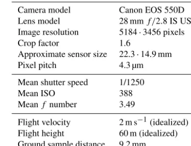
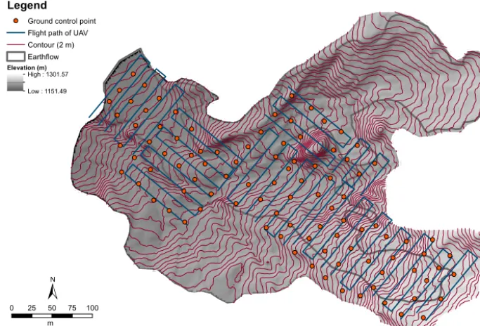
In order to provide a spatial analysis of surface deformation through time, a time series of very high-resolution datasets of the Schimbrig area is necessary. Given the high geomor-phic activity in the area (Schwab et al., 2008), yearly sur-veys were planned to accurately capture earthflow move-ments at high temporal resolution. Three image acquisition campaigns were organized in October 2013, June 2014, and October 2015. Late summer and late spring periods were chosen in order to minimize the effects of vegetation growth. Image acquisition is done using a UAV platform, i.e. a custom Y6 multirotor with embedded DJI controllers. It is equipped with a stabilized camera mount, which compen-sates for tilt and roll movements to maintain the fixed ori-entation of the camera. The used camera is a standard small-format (i.e. 18.0 effective megapixel CMOS APS-C sensor) reflex camera (Canon EOS 550D). The lens is a fixed-focal-length lens (Canon EF 28 mmf/2.8 IS USM), equipped with an optical image stabilizer and a high-speed autofocus mo-torization. The ground surface is surveyed both with nadir-oriented and with a 45◦-tilted camera, as the inclusion of oblique images in the SfM algorithm has been shown to de-crease systematic errors in topographic reconstruction and to better capture complex 3-D structures (Clapuyt et al., 2016; James and Robson, 2014). Given a mean speed of 2 m s−1to
avoid motion blur induced by the UAV platform, the acquisi-tion frequency is set at a rate of one image per 2 s in order to have a high overlap between consecutive images at ca. 60 m above ground, i.e. above 70 %, because high redundancy im-proves the performance of the SfM algorithm. Adjacent flight lines are separated by 15 m to maintain high lateral overlap of aerial images (Fig. 2). Even though image acquisition has
Table 1.Camera and imaging characteristics for all the surveys.
Camera model Canon EOS 550D
Lens model 28 mmf/2.8 IS USM
Image resolution 5184·3456 pixels
Crop factor 1.6
Approximate sensor size 22.3·14.9 mm
Pixel pitch 4.3 µm
Mean shutter speed 1/1250
Mean ISO 388
Meanf number 3.49
Flight velocity 2 m s−1(idealized)
Flight height 60 m (idealized)
Ground sample distance 9.2 mm
been performed in diverse light conditions depending on the hour of the day and cloud coverage during flights, the bot-tom line has always been to shoot in shutter speed priority mode and maintain a high value to avoid motion blur. Cam-era, flight, and imaging parameters are summarized in Ta-ble 1 (O’Connor et al., 2017).
sedi-±
0 25 50 75 100
Legend Ground control point Flight path of UAV Contour (2 m) Earthflow Elevation (m)
High : 1301.57
Low : 1151.49
m
Figure 2.Settings of the UAV flights and GCP location (example from the October 2015 survey).
ment budget and horizontal displacements. The resolution of the outputs was set based on the average density of 3-D point clouds and standardized for all the datasets.
To quantify internal deformation of the Schimbrig earth-flow, three distinct and complementary analyses are realized on the time series of 3-D point clouds. First, the sediment budget is evaluated by computing DoD between DSMs, us-ing the Geomorphic Change Detection software (Wheaton et al., 2010). Uncertainties associated with each surface repre-sentation, i.e. the accuracy values of 3-D point clouds, are considered to be uniform over the entire study area. We sub-sequently analyse thresholded DSMs. The errors on the to-pographic representations are then propagated in the calcu-lations of the DoD and quantities of erosion and deposition. By computing differences between DSMs, the mass balance of the earthflow is derived from the difference between the total eroded volume and the total deposited volume of sedi-ments. Additionally, the average net thickness difference in elevation is computed by dividing the net volume difference by the surface area of the earthflow.
Second, horizontal surface displacements are computed using the COSI-Corr image correlation algorithm (Ayoub et al., 2009; Leprince et al., 2007). Correlation is computed based on a moving window that scans dataset pairs. We used pairs of shaded relief surfaces to detect horizontal displace-ments. This method is particularly suitable for monitoring slow deformation processes, like the Schimbrig earthflow, with clearly distinguishable surface deformation structures, such as cracks, fissures, and scarps. The COSI-Corr algo-rithm results in horizontal displacements expressed as two layers, i.e. the north–south component and the east–west
component, which are combined to compute the intensity and direction of ground movements. The horizontal displace-ment analysis is compledisplace-mentary to the above-displace-mentioned 3-D analysis of point clouds: the presence of micro-topography and vegetation in the 3-D point clouds facilitates the quan-tification of lateral earth movements using the COSI-Corr al-gorithm. As such, the complexity of the earthflow including erosion and accumulation areas and horizontal displacements of the earthflow body is better represented. For each time interval, descriptive statistics, i.e. minimum, mean, median, quartile, and maximum, are computed for the distribution of horizontal displacement values.
in-±
0 25 50 75 100 m
Legend Earthflow Intersection 2013–2014 Intersection 2014–2015
Figure 3.Intersections of point cloud datasets for the 2013–2014 and 2014–2015 time intervals.
terval allows distinguishing statistically significant changes between two point clouds (Lague et al., 2013). Again, sim-ple descriptive statistics are computed on the distribution of local distances between point clouds for each time interval.
The SfM processing and 3-D point cloud georeferencing are performed using the Agisoft Photoscan®software. Sedi-ment budgets were computed with the Geomorphic Change Detection software implemented in ArcGIS. COSI-Corr al-gorithm has been used as a software module integrated in ENVI. Point cloud handling has been done with CloudCom-pare, using the M3C2 plugin. All other data manipulations were carried out with R software, CloudCompare, and Ar-cGIS 10.
3 Results
3.1 3-D topographic reconstructions
The three topographic reconstructions are not covering the same spatial domain (Table 2; Fig. 3). The flight campaign of June 2014 allowed us to survey the entire Schimbrig earth-flow. The 2013 and 2015 flight campaigns are centred on the most active part of the earthflow but do not cover the en-tire earthflow due to operational problems encountered dur-ing flights.
Due to these spatial limitations, results are presented: (1) over the spatial intersection of the three datasets (T2013
T
T2014 TT2015), i.e. area of interest namedintersection,
to allow the comparison of absolute values of displacement and volumetric changes over the entire time period (2013– 2015), and (2) over the spatial intersection of each time
in-terval (T2013TT2014andT2014TT2015), i.e. area of interest
referred to asinterval, in order to get the most information of each pair of datasets.
The 3-D point cloud reconstructions of the Schimbrig earthflow result in a large dataset, with a very high point den-sity of ca. 1000 to 1450 points per square metre, which al-lows accurate tracking of ground deformation through time. The three topographic reconstructions have similar accura-cies, i.e. RMSE (Table 2), with horizontal accuracies of 0.23 and 0.20 m, and vertical accuracies of 0.06, 0.05, and 0.08 m. The total error on the topographic reconstructions ranges between 0.20 and 0.24 m. The overall detection limits for ground movements and deformations are derived from er-ror propagation of the RMSE values on the individual topo-graphic constructions given in Table 2.
The detection limits are similar for the two time inter-vals (Table 3), with a value of 0.31 m for 2013–2014 and 0.30 m for 2014–2015. For further analyses, changes which are smaller than the detection limit of our UAV-SfM frame-work are not reported.
3.2 Geomorphological map
sta-Table 2.Characteristics and accuracy assessment of 3-D point cloud reconstructions. Root mean square errors (RMSE) are the standard de-viation of differences between the coordinates of the ground control points, i.e. georeferencing targets, measured by GPS and the coordinates of these points within the 3-D point clouds after georeferencing. Horizontal RMSE is computed by taking the horizontal components of the point coordinates, while the vertical RMSE is computed by taking only thezcomponent of point coordinates.
October 2013 June 2014 October 2015
Point cloud characteristics No. of pictures 1143 4519 2501
No. of GCPs 49 108 99
Area (ha) 5.86 17.69 15.59
Point density (pts m−2) 1456 1270 1080
RMSE (m) Horizontal 0.23 0.20 0.20
Vertical 0.06 0.05 0.08
Total error 0.24 0.20 0.22
±
0 25 50 75 100 m
Legend Earthflow Geomorphological units
Earthflow - Accumulation zone Earthflow
Earthflow covered with pasture Erosional escarpment Gorge
Soil mantled ridge Gentle slope
Figure 4.Geomorphological map of the study area.
Table 3.Limit-of-detection values for temporal analyses (metres).
2013–2014 2014–2015
Limit of detection (m) Horizontal 0.30 0.28
Vertical 0.08 0.09
Total 0.31 0.30
ble ridges and visual analysis of geomorphic units are based on expert knowledge.
The Schimbrig earthflow is constrained by stable bedrock ridges covered by trees on the northeastern part, and by rel-atively stable grasslands on the southwestern part. The main track of the earthflow is from the southeast to the northwest,
and it contains two scarps in the upper part that expose up to 25 m. The earthflow is characterized by a rough surface and a patchwork of vegetated surfaces covered by herbs and small shrubs and bare surfaces where wet and bare soil (silt and mud with embedded clasts) is exposed. The secondary track flows from the northeast to southwest and joins the main track upslope of its accumulation zone.
3.3 Sediment budget
Table 4.Volumetric (cubic metres) and depth (metres) sediment budgets.
Area of interest Intersection Interval
Time interval 2013–2014 2014–2015 2014–2015
Estimate Error (±) Estimate Error (±) Estimate Error (±)
Total volume of erosion (m3) −11 345 3118 −9054 2329 −15 093 4098
Total volume of deposition (m3) 6012 1919 8293 2546 17 005 4533
Total net volume of difference (m3) −5333 3661 −762 3450 1912 6111
Average net thickness difference (m) −0.22 0.15 −0.03 0.14 0.05 0.15
Figure 5.Volumetric sediment budget computed for the spatial
in-tersection of the three datasets (see Table 4 for details).
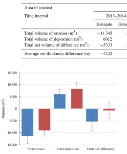
applied to each input dataset as defined in Table 2. Over the intersection of the surveyed areas, the estimated volume of deposited material is 6012±1919 m3, for the first period of interest, i.e. between October 2013 and June 2014 (Table 4; Fig. 5). The volume of eroded material is larger, with an es-timate of−11 345±3118 m3. For the first period, there is a net negative change in volume indicating that the removal of material is larger than the accumulation of sliding material for the surveyed surfaces. On average, there is lowering of the surface of 0.22±0.15 m (Table 4). Field observations re-veal a similar pattern. It is important to note that the lower part of the earthflow, where the debris is accumulating in a frontal lobe, is not included in the topographic analyses. Field observations indicate that only a minor part of the slid-ing material might have been transported to the river network via the Rossloch River.
The sediment budget computed over the second time in-terval, i.e. between June 2014 and October 2015, for the area of intersection is nearly at equilibrium (Table 4; Fig. 5) with a net volume of difference of−762 m3±3450 m3. This suggests that the sliding material that is mobilized by the earthflow accumulated within the area of intersection. When analysing the internal flow dynamics of the larger sliding area
(interval) over the second time interval, it is clear that the sediment budget is slightly positive (Table 4). This analy-sis now also captures the frontal lobe of the mass movement that bulged and advanced during this time interval. Figure 6 also shows that the upper and lower part of the earthflow are bulging areas, while the intermediate zone is experiencing surface subsidence.
3.4 Horizontal displacements
The COSI-Corr image correlation algorithm uses pairs of single-band input to quantify horizontal displacement. A north-directed illumination on the DSMs allows for high-lighting topographic features and ground deformation prop-erly, as well as the presence of low vegetation. Shaded relief surfaces derived from the 3-D point clouds (with a spatial resolution of 0.2 m) provided the best results for the correla-tion analyses. It is important to mencorrela-tion that input data with smaller spatial resolution generated incoherent displacement results, associated with high signal-to-noise ratio. In fact, un-der 0.2 m resolution, image correlation led to false positive correlation between features due to the very complex topog-raphy of the earthflow. Pixels characterized by a signal-to-noise ratio lower than 0.9 or by displacement vectors that are smaller than the detection threshold are discarded for further analyses. To allow comparison between the two time inter-vals that have a different duration, i.e. 8 versus 17 months, the displacement values are here represented as mean annual displacement values (Table 5).
For the period between October 2013 and June 2014, the fluxes are relatively high and well confined by stable mor-phologic ridges surrounding the earthflow (Fig. 7). The dis-placement pattern is rather uniform over the entire length of the earthflow, suggesting that the earthflow body is mov-ing downslope between stable bedrock ridges. The zones that show higher sliding activity are the lower scarp of the earth-flow and its adjacent flat slope. The mean annual horizontal displacement for this first period is about 8.9 m.
±
0 20 40 60 80 m
Legend
Elevation difference (m)
-13.2 12 -11.9 10 -9.9 8 -7.99 6 -5.99 4 -3.99 2 -1.99 0.30 0.30 2 2.01 4 4.01 6 6.01 8 8.01 10 10.1 12 – – –
– – – – – – – – – –
Figure 6.Elevation difference between two topographic reconstructions for the time interval June 2014–October 2015.
±
0 25 50 75 100 m
2013 – 2014 Displacement vector Meanannualdisplacement(m)
0.5 - 1.6 1.7 - 2.2 2.3 - 9.2 9.3 - 13.5 13.6 - 40.2
Figure 7.Surface displacements for 2013–2014 using the COSI-Corr algorithm. Displacement vectors are indicative of relative magnitude
and direction of movement and do not reflect true ground displacements.
scarps in the upper part, in the secondary track of the earth-flow, and in the lower accumulation zone where the frontal lobe spectacularly advanced downslope. In the flatter area between the two scarps, the horizontal movement is less pro-nounced and the direction of movement is rather diffuse.
When comparing the surface displacements for the two time periods over the same study area, it is clear that the
mag-nitude of the horizontal displacements is lower in the second period with a mean annual displacement of 5.7 m.
±
0 25 50 75 100 m
2014–2015
Displacement vector Meanannualdisplacement(m)
0.2 - 1.6 1.7 - 2.2 2.3 - 9.2 9.3 - 13.5 13.6 - 21.1
Figure 8.Surface displacements for 2014–2015 using the COSI-Corr algorithm. Displacement vectors are indicative of relative magnitude
and direction of movement and do not reflect true ground displacements.
Table 5.Mean annual horizontal displacement (metres) computed
using the COSI-Corr algorithm applied on shaded relief surfaces.
Area of interest Intersection Interval
Time interval 2013–2014 2014–2015 2014–2015
Min. 0.47 0.23 0.23
1st Q. 1.81 0.89 0.89
Median 3.74 2.20 3.62
Mean 8.91 5.74 6.30
3rd Q. 13.06 11.25 11.84
Max. 40.16 21.06 21.06
ridges constrain the direction of the earthflow movement. Although the spatial pattern is highly consistent, the abso-lute displacement of the frontal lobe of the earthflow is not properly captured, as the frontal lobe advanced by ca. 55 m (Fig. 9).
3.5 3-D comparison of earth topography
Distances between 3-D point clouds are computed using the M3C2 algorithm. For each pair of point cloud datasets, a sub-sample of the first 3-D point cloud is taken as the set of core points, with a minimum distance of 0.5 m between points, to avoid extensive computation time. Descriptive statistics are computed on the point cloud distances (Table 6) which were filtered from values under the detection threshold.
The dominance of negative values can be interpreted as predominance of ground subsidence in flat parts or scarp re-treat in steeper areas of the earthflow. Contrariwise, positive
Table 6.Descriptive statistics of the distances between 3-D point
clouds (metres).
Area of interest Intersection Interval
Time interval 2013–2014 2014–2015 2014–2015
Min. −20.72 −27.56 −28.83
1st Q. −1.06 −1.00 −0.89
Median −0.60 −0.49 −0.43
Mean −1.04 −0.69 −0.38
3rd Q. 0.47 0.66 0.79
Max. 20.36 26.96 26.96
values are zones of surface bulging in the zones of accumu-lation or accumuaccumu-lation of debris at the frontal lobe.
4 Discussion
4.1 Application of UAV-SfM framework for landslide monitoring
advan-Figure 9.Aerial images illustrating the advance of the frontal lobe of the earthflow between June 2014 and October 2015.
tages of the UAV-SfM framework are its flexibility and its low cost and light weight, which are convenient for repeated measurements of dynamic environments, and more particu-larly when deployed to acquire aerial imagery in remote and poorly accessible areas. Similar to terrestrial laser scanning, which has similar spatial accuracy and range, the UAV-SfM framework requires careful setup and planning of georefer-encing targets and image acquisition to adequately and accu-rately capture the 3-D scene of complex topography (Caduff et al., 2015; Clapuyt et al., 2016; James et al., 2017b). Be-ing an airborne acquisition platform, the UAV-SfM has the advantage of configuring a dense network of optimal view-points independent of terrain complexity and access difficul-ties.
The workflow applied for the research is based on our previous work on reproducibility of the technique (Clapuyt et al., 2016). The use of ground control points is time-consuming for large areas, as it requires a sufficient num-ber of observations that are well distributed around the study area. However, both criteria were fulfilled in our surveys. Only some GCPs, i.e. less than 5 %, were discarded from the analysis because of the important associated error on the GPS measurement. Consequently, the use of the GCP geo-referencing technique does not significantly affect our re-sults, as observations were not included in the bundle adjust-ment step. However, we are confident that direct georeferenc-ing technique for UAV-SFM framework will soon become a standard procedure as compact and low-cost real-time kine-matic (RTK) receivers are now available and suitable to be embedded on UAV platforms. Performance of direct geo-referencing has recently been assessed and showed to be at least similar to GCP georeferencing (Carbonneau and Diet-rich, 2017; James et al., 2017a). In fact, this technique in-creases the field survey efficiency as the amount of GCPs can be significantly reduced and more importantly, it will in-crease the accuracy of topographic reconstructions where ac-cessibility to place GCPs is drastically limited, e.g. volcanic terrains and glaciers. For further surveys of the Schimbrig earthflow, our workflow has to be adapted to include direct georeferencing. In this case study, a 1-year time interval
be-tween surveys was suitable to capture the internal dynamics of the earthflow (Schwab et al., 2007). With respect to this, our 3-D temporal database is considered as dense. We rec-ognize that other natural hazards may require a higher fre-quency of measurements, which can easily be achieved using UAVs. Even though our results about landslide structure and dynamics need to be viewed against geophysical or geotech-nical field investigations, this study shows the potential of time series of UAV-SfM topographic reconstructions to pro-vide complementary data on internal landslide dynamics in complex terrain.
One of the main drawbacks of the UAV-SfM framework is the need for the UAV platform to acquire aerial pictures. The use of UAVs is now increasingly subjected to more strin-gent regulations, including a pilot license, UAV registration, and insurance certificates (Stöcker et al., 2017). Moreover, UAV flights are only possible under optimal meteorological conditions, and wind and rain may be a limiting factor in mountainous areas.
4.2 Schimbrig earthflow monitoring
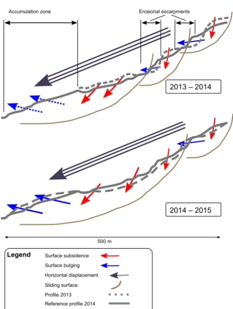
Post-processing of the time series of DSMs provides sed-iment budgets, horizontal displacements and 3-D compar-isons of surfaces that allow us to monitor the internal dy-namics of the mass movement at very high spatial and tem-poral resolution. By qualitatively combining quantitative sin-gle results, which may initially seem redundant, it is possible to quantify the magnitude and rate of sediment redistribu-tion and surface movements within the area affected by the Schimbrig earthflow and more importantly to capture the in-ternal mechanisms of the earthflow (Fig. 10).
2013 – 2014
2014 – 2015
Accumulation zone Erosional escarpments
500 m
12
0
m
Surface subsidence Surface bulging
Legend
Profile 2013 Horizontal displacement Sliding surface
Reference profile 2014 Profile 2015
Figure 10. Schematic summary of the internal dynamics of the
Schimbrig earthflow based on very high-resolution monitoring us-ing the UAV-SfM framework.
of photogrammetric techniques, but the temporal informa-tion has its limits regarding quantitative and continuous data on displacement rates. A first attempt to quantify slip rates of the earthflow was carried out by Schwab et al. (2007), who tracked control points using GPS measurements. How-ever, we are now able to compute slip rates over the entire extent of the earthflow at very high temporal resolution ap-plying image correlation algorithms to very high-resolution aerial images. Schwab et al. (2008) complemented their to-pographic analysis of the earthflow using classic photogram-metry and aerial photographs spanning the last 50 years. In-dependent of the spatial resolution of the output and price of data acquisition, photogrammetric analyses are very valuable as they allow for capturing surface displacements on larger scales and over longer time periods than data derived from the UAV-SfM framework, even though the time interval be-tween the data sets may be a limiting factor (e.g. Prokešová et al., 2010; van Westen and Lulie Getahun, 2003). Schwab et al. (2008) emphasized that sediment fluxes in the trunk streams are not directly controlled by the production of loose material through landsliding on the hillslopes. This is con-firmed by our high-resolution topographic analysis and the computed hillslope sediment budget.
The UAV-SfM framework allows one to go a step further in the interpretation of the earthflow’s internal structure and dynamics.
When superimposing the temporal series of the three sets of topographic analyses and interpreting it in very detailed way, we are able to show the complex rotational structure of the earthflow (Fig. 10). Our data show that the entire body of the earthflow is sliding but that there exist strong differences in internal deformation and flow velocities within the sliding material. By combining the results from the 3-D comparison between the point clouds and the DoD, it is possible to map the succession of ground surface subsidence and bulging ar-eas over the 3-year period. Notwithstanding the short mon-itoring interval, the pattern of internal deformation of the earthflow changed its configuration (Fig. 10). Between Oc-tober 2013 and June 2014, the earthflow had a succession of three nested rotational units. In the upper part of the study area, two steep scarps are present. These active scarps con-trol the downward movement of two tilted blocks (see Fig. 4). The location of the two main scarps advances by ca. 8 m dur-ing the 2013–2014 period. A third rotational unit is larger: it is defined by a steep scarp located in the middle part of the earthflow and extends over the lower and flatter part of the earthflow down the frontal lobe.
During the second period of monitoring, i.e. between June 2014 and October 2015, two rotational units can clearly be distinguished, i.e. a small upper block that is confined above the upper active scarp and a larger heterogeneous slid-ing mass that extends down to the frontal lobe of the earth-flow. Unlike the first period of interest, the lower erosional scarp is not active, and there is no distinction between the second and third part of the sliding mass.
The very high-resolution spatio-temporal analyses demon-strate that the Schimbrig earthflow was very active over the monitoring period. Results from the image correlation algo-rithm highlight the strong internal redistribution of sliding material within the earthflow, as well as rapid changes in the spatial pattern of displacement vectors. The mean an-nual horizontal displacements are large, with values of ca. 9 m between October 2013 and June 2014 and ca. 6 m be-tween June 2014 and October 2015. This is partly explained by the fact that the central part of the earthflow is advanc-ing toward the foot of the earthflow between October 2013 and June 2014, and this advance is accompanied by surface subsidence along the main track. This phase is followed by bulging in the accumulation zone, and a strong advance of the frontal lobe of the landslide over a distance of ca. 55 m.
earth-flow (Schwab et al., 2008). More than 20 years later, the earthflow shows strong internal deformation that is related to the re-adjustment and self-reorganization of the sliding ma-terial after the 1994 surge event. This suggests that phases of enhanced earthflow kinematics are not necessarily leading to enhanced sediment export to the fluvial system, as a result of the time delay between successive phases of earthflow reac-tivation and the sediment export from the catchment.
5 Conclusion
The UAV-SfM framework is increasingly applied in geo-morphology to accurately capture the topography of given scenes. As it is low-cost and flexible in its implementa-tion, and particularly suitable for surveying dynamic environ-ments in poorly accessible terrain, we used this methodology to quantify ground surface displacements of the Schimbrig earthflow, located at the foothills of the Central Swiss Alps, at very high spatial and temporal resolution. Based on three topographic reconstructions between autumn 2013 and 2015, we were able to conduct a comprehensive 3-D analysis of the landslide by combining the sediment budget of the hillslope as well as the horizontal and the three-dimensional surface displacements.
Combination and careful interpretation of the three topo-graphic analyses of this study allow us to reconstruct the in-ternal dynamics of the earthflow and highlight its complex rotational movement. In addition to variation in horizontal surface movements through time, we interestingly showed that the rotational structure of the earthflow is also vary-ing from year to year. Additional field surveys will be re-quired to increase the temporal series of topography recon-structions and confirm our findings. Results also confirm that the Schimbrig earthflow is very active, with mean annual hor-izontal displacements between 6 and 9 m. Furthermore, we showed that the sediment budget of the hillslope is nearly at equilibrium. In fact, the earthflow experienced a major sed-iment pulse more than 20 years ago and is still re-adjusting to this new setting. Therefore, our very high spatial and tem-poral resolution analysis supports the findings of Schwab et al. (2008) about the time lag between sediment production on hillslopes and fluvial processes, i.e. enhanced sediment fluxes, in trunk streams, based on lower spatial and temporal resolution time series of DEMs. Finally, this short-term mon-itoring of the Schimbrig earthflow is a good addition to the previous studies done over the same study area. It provides additional value in allowing further research, which will in-tegrate all of these spatial and temporal scales in terms of erosion and hillslope processes.
Data availability. The data for this paper are available by
contact-ing Veerle Vanacker at the Department of Geography, University of Louvain, Place Louis Pasteur, 1348 Louvain-la-Neuve, Belgium ([email protected]).
Competing interests. The authors declare that they have no
con-flict of interest.
Special issue statement. This article is part of the special issue
“4-D reconstruction of earth surface processes: multi-temporal and multi-spatial high resolution topography”. It is not associated with a conference.
Acknowledgements. The authors would like to thank
Emi-lien Aldana Jague and Marco Bravin for the help and the support during test flights with the UAVs used to acquire aerial images. We would also like to acknowledge Romain Delunel from Bern University for its availability and help regarding the handling of the GPS used to survey ground control points during field work. Furthermore, authors thank the two anonymous reviewers and the handling associate editor, Anette Eltner, for their constructive com-ments. Low-cost research is also possible thanks to the developers making their software freely available: Dimitri Lague and Nico-las Brodu for the M3C2 algorithm; the COSI-Corr development team, from Caltech (California Institute of Technology) Tectonics Observatory; and Joe Wheaton and colleagues for the Geomorphic Change Detection software.
Edited by: Anette Eltner
Reviewed by: two anonymous referees
References
Ayoub, F., Leprince, S., and Avouac, J.-P.: Co-registration and correlation of aerial photographs for ground deformation mea-surements, ISPRS J. Photogramm. Remote Sens., 64, 551–560, https://doi.org/10.1016/j.isprsjprs.2009.03.005, 2009.
Bennett, G. L., Molnar, P., McArdell, B. W., Schlunegger, F., and Burlando, P.: Patterns and controls of sediment production, trans-fer and yield in the Illgraben, Geomorphology, 188, 68–82, https://doi.org/10.1016/j.geomorph.2012.11.029, 2013. Blasone, G., Cavalli, M., Marchi, L., and Cazorzi, F.:
Mon-itoring sediment source areas in a debris-flow
catch-ment using terrestrial laser scanning, Catena, 123, 23–36, https://doi.org/10.1016/j.catena.2014.07.001, 2014.
Caduff, R., Schlunegger, F., Kos, A., and Wiesmann, A.: A re-view of terrestrial radar interferometry for measuring surface change in the geosciences, Earth Surf. Proc. Land., 40, 208–228, https://doi.org/10.1002/esp.3656, 2015.
Casson, B., Delacourt, C., Baratoux, D., and Allemand, P.: Sev-enteen years of the “La Clapière” landslide evolution analysed from ortho-rectified aerial photographs, Eng. Geol., 68, 123–139, https://doi.org/10.1016/S0013-7952(02)00201-6, 2003. Clapuyt, F., Vanacker, V., and Van Oost, K.:
Reproducibil-ity of UAV-based earth topography reconstructions based on Structure-from-Motion algorithms, Geomorphology, 260, 4–15, https://doi.org/10.1016/j.geomorph.2015.05.011, 2016. Crozier, M. J.: Deciphering the effect of climate change on
landslide activity: A review, Geomorphology, 124, 260–267, https://doi.org/10.1016/j.geomorph.2010.04.009, 2010. Cubasch, U., Wuebbles, D., Chen, D., Facchini, M. C.,
Frame, D., Mahowald, N., and Winther, J.-G.:
Intro-duction in Climate Change 2013, Intergov. Panel Clim. Chang. 2013 Phys. Sci. Basis. Contrib. Work. Gr. I to Fifth Assess. Rep. Intergov. Panel Clim. Chang., 119–158, https://doi.org/10.1017/CBO9781107415324.007, 2013. Delacourt, C., Allemand, P., Casson, B., and Vadon, H.: Velocity
field of the “La Clapière” landslide measured by the correlation of aerial and QuickBird satellite images, Geophys. Res. Lett., 31, 1–5, https://doi.org/10.1029/2004GL020193, 2004.
Eltner, A., Kaiser, A., Castillo, C., Rock, G., Neugirg, F., and Abel-lán, A.: Image-based surface reconstruction in geomorphometry – merits, limits and developments, Earth Surf. Dynam., 4, 359-389, https://doi.org/10.5194/esurf-4-359-2016, 2016.
Fernández, T., Pérez, J. L., Cardenal, J., Gómez, J. M., Colomo, C., and Delgado, J.: Analysis of landslide evolution affecting olive groves using UAV and photogrammetric techniques, Re-mote Sens., 8, 837, https://doi.org/10.3390/rs8100837, 2016. Fressard, M., Maquaire, O., Thiery, Y., Davidson, R., and
Lissak, C.: Geomorphology Multi-method characterisation of an active landslide: Case study in the Pays d’Auge plateau (Normandy, France), Geomorphology, 270, 22–39, https://doi.org/10.1016/j.geomorph.2016.07.001, 2016. Guns, M. and Vanacker, V.: Shifts in landslide frequency–area
dis-tribution after forest conversion in the tropical Andes, Anthro-pocene, 6, 75–85, https://doi.org/10.1016/j.ancene.2014.08.001, 2014.
Hervás, J., Barredo, J. I., Rosin, P. L., Pasuto, A., Mantovani, F., and Silvano, S.: Monitoring landslides from optical remotely sensed imagery: The case history of Tessina landslide, Italy,
Geomorphology, 54, 63–75,
https://doi.org/10.1016/S0169-555X(03)00056-4, 2003.
Huang, H., Long, J., Lin, H., Zhang, L., Yi, W., and Lei, B.: Unmanned aerial vehicle based remote sensing method for monitoring a steep mountainous slope in the Three Gorges Reservoir, China, Earth Sci. Inform., 10, 287–301, https://doi.org/10.1007/s12145-017-0291-9, 2017.
Huggel, C., Clague, J. J., and Korup, O.: Is climate change respon-sible for changing landslide activity in high mountains?, Earth Surf. Proc. Land., 37, 77–91, https://doi.org/10.1002/esp.2223, 2012.
Immerzeel, W. W., Kraaijenbrink, P. D. A., Shea, J. M., Shrestha, A. B., Pellicciotti, F., Bierkens, M. F. P., and de Jong, S. M.: High-resolution monitoring of Himalayan glacier dynamics us-ing unmanned aerial vehicles, Remote Sens. Environ., 150, 93– 103, https://doi.org/10.1016/j.rse.2014.04.025, 2014.
Jaboyedoff, M., Oppikofer, T., Abellán, A., Derron, M.-H., Loye, A., Metzger, R., and Pedrazzini, A.: Use of LIDAR
in landslide investigations: a review, Nat. Hazards, 61, 5–28, https://doi.org/10.1007/s11069-010-9634-2, 2012.
James, M. R. and Robson, S.: Mitigating systematic error in topographic models derived from UAV and ground-based image networks, Earth Surf. Proc. Landf., 39, 1413–1420, https://doi.org/10.1002/esp.3609, 2014.
James, M. R., Robson, S., and Smith, M. W.: 3-D uncertainty-based topographic change detection with structure-from-motion pho-togrammetry: Precision maps for ground control and directly georeferenced surveys, Earth Surf. Proc. Land., 42, 1769–1788, https://doi.org/10.1002/esp.4125, 2017a.
James, M. R., Robson, S., d’Oleire-Oltmanns, S., and Ni-ethammer, U.: Optimising UAV topographic surveys pro-cessed with structure-from-motion: Ground control quality, quantity and bundle adjustment, Geomorphology, 280, 51–66, https://doi.org/10.1016/j.geomorph.2016.11.021, 2017b. Joyce, K. E., Belliss, S. E., Samsonov, S. V., McNeill, S. J.,
and Glassey, P. J.: A review of the status of satellite remote sensing and image processing techniques for mapping natu-ral hazards and disasters, Prog. Phys. Geogr., 33, 183–207, https://doi.org/10.1177/0309133309339563, 2009.
Kääb, A.: Monitoring high-mountain terrain deformation from repeated air-and spaceborne optical data: examples using dig-ital aerial imagery and ASTER data, ISPRS J. Photogramm.
Remote Sens., 57, 39–52,
https://doi.org/10.1016/S0924-2716(02)00114-4, 2002.
Lague, D., Brodu, N., and Leroux, J.: Accurate 3D
com-parison of complex topography with terrestrial laser
scanner: Application to the Rangitikei canyon
(N-Z), ISPRS J. Photogramm. Remote Sens., 82, 10–26,
https://doi.org/10.1016/j.isprsjprs.2013.04.009, 2013.
Lateltin, O., Haemmig, C., Raetzo, H., and Bonnard, C.: Land-slide risk management in Switzerland, LandLand-slides, 2, 313–320, https://doi.org/10.1007/s10346-005-0018-8, 2005.
Leprince, S., Barbot, S., Ayoub, F., and Avouac, J.: Automatic and precise orthorectification, coregistration, and subpixel correla-tion of satellite, images, applicacorrela-tion to ground deformacorrela-tion mea-surements, IEEE T. Geosci. Remote Sens., 45, 1529–1558, 2007. Lucieer, A., de Jong, S. M., and Turner, D.: Mapping landslide dis-placements using Structure from Motion (SfM) and image corre-lation of multi-temporal UAV photography, Prog. Phys. Geogr., 38, 97–116, https://doi.org/10.1177/0309133313515293, 2014. Merritt, A. J., Chambers, J. E., Murphy, W., Wilkinson, P. B.,
West, L. J., Gunn, D. A., Meldrum, P. I., Kirkham, M., and Dixon, N.: 3D ground model development for an ac-tive landslide in Lias mudrocks using geophysical, remote sensing and geotechnical methods, Landslides, 11, 537–550, https://doi.org/10.1007/s10346-013-0409-1, 2014.
Metternicht, G., Hurni, L., and Gogu, R.: Remote sens-ing of landslides: An analysis of the potential contribu-tion to geo-spatial systems for hazard assessment in moun-tainous environments, Remote Sens. Environ., 98, 284–303, https://doi.org/10.1016/j.rse.2005.08.004, 2005.
D. G., Wasklewicz, T., and Wheaton, J. M.: Analyzing high res-olution topography for advancing the understanding of mass and energy transfer through landscapes: A review, Earth-Sci. Rev., 148, 174–193, https://doi.org/10.1016/j.earscirev.2015.05.012, 2015.
Perrone, A., Lapenna, V., and Piscitelli, S.: Earth-Science Re-views Electrical resistivity tomography technique for land-slide investigation?: A review, Earth-Sci. Rev., 135, 65–82, https://doi.org/10.1016/j.earscirev.2014.04.002, 2014.
Peternel, T., Kumelj, Š., Oštir, K., and Komac, M.: Monitoring the Potoška planina landslide (NW Slovenia) using UAV photogram-metry and tachymetric measurements, Landslides, 14, 395–406, https://doi.org/10.1007/s10346-016-0759-6, 2017.
Prokešová, R., Kardoš, M., and Medved’ová, A.: Landslide dynam-ics from high-resolution aerial photographs: A case study from the Western Carpathians, Slovakia, Geomorphology, 115, 90– 101, https://doi.org/10.1016/j.geomorph.2009.09.033, 2010. Raetzo, H., Lateltin, O., Bollinger, D., and Tripet, J. P.:
Haz-ard assessment in Switzerland – Codes of practice for mass movements, B. Eng. Geol. Environ., 61, 263–268, https://doi.org/10.1007/s10064-002-0163-4, 2002.
Raucoules, D., de Michele, M., Malet, J. P., and Ulrich, P.: Time-variable 3D ground displacements from high-resolution syn-thetic aperture radar (SAR). application to La Valette landslide (South French Alps), Remote Sens. Environ., 139, 198–204, https://doi.org/10.1016/j.rse.2013.08.006, 2013.
Rippin, D. M., Pomfret, A., and King, N.: High resolution map-ping of supra-glacial drainage pathways reveals link between micro-channel drainage density, surface roughness and sur-face reflectance, Earth Surf. Proc. Landforms, 40, 1279–1290, https://doi.org/10.1002/esp.3719, 2015.
Savi, S., Schneuwly-Bollschweiler, M., Bommer-Denns, B., Stof-fel, M., and Schlunegger, F.: Geomorphic coupling between hill-slopes and channels in the Swiss Alps, Earth Surf. Proc. Land., 38, 959–969, https://doi.org/10.1002/esp.3342, 2013.
Scaioni, M., Longoni, L., Melillo, V., and Papini, M.: Remote-sensing for landslide investigations: An overview of recent achievements and perspectives, Remote Sens., 6, 9600–9652, https://doi.org/10.3390/rs6109600, 2014.
Schlögel, R., Doubre, C., Malet, J. P., and Masson, F.:
Landslide deformation monitoring with ALOS/PALSAR
imagery: A D-InSAR geomorphological
interpre-tation method, Geomorphology, 231, 314–330,
https://doi.org/10.1016/j.geomorph.2014.11.031, 2015. Schlunegger, F., Jost, J., Grünig, A., and Trüssel, M.:
Er-läuterungen, Geologischer Atlas der Schweiz, Kartenblatt 1169 Schüpfheim 1 : 25’000, Bundesamt für Landestopographie swis-stopo, 107 pp., 2016a.
Schlunegger, F., Anspach, O., Bieri, B., Böning, P., Kaufmann, Y., Lahl, K., Lonschinski, M., Mollet, H., Sachse, D., Schubert, C., Stöckli, G., and Zander, I.: Geologische Karte der Schweiz, Kartenblatt 1169 Schüpfheim 1 : 25’000, Bundesamt für Lan-destopographie swisstopo, 2016b.
Schwab, M., Läderach, C., Rieke-Zapp, D., and Schlunegger, F.: Slip rates variability and sediment mobilization on a shallow landslide in the northern Swiss Alps, Swiss J. Geosci., 100, 281– 292, https://doi.org/10.1007/s00015-007-1218-0, 2007. Schwab, M., Rieke-Zapp, D., Schneider, H., Liniger, M., and
Schlunegger, F.: Landsliding and sediment flux in the
Cen-tral Swiss Alps: A photogrammetric study of the Schim-brig landslide, Entlebuch, Geomorphology, 97, 392–406, https://doi.org/10.1016/j.geomorph.2007.08.019, 2008. Seijmonsbergen, A. C.: The modern geomorphological map, in:
Treatise on Geomorphology, edited by: Shroder, J. F., 35–52, Academic Press, San Diego, 2013.
Seneviratne, S. I., Corti, T., Davin, E. L., Hirschi, M., Jaeger, E. B., Lehner, I., Orlowsky, B., and Teuling, A. J.: Investigating soil moisture-climate interactions in a changing climate: A review, Earth-Sci. Rev., 99, 125–161, https://doi.org/10.1016/j.earscirev.2010.02.004, 2010.
Smith, M. W., Carrivick, J. L., and Quincey, D. J.: Structure from motion photogrammetry in physical geography, Prog. Phys. Ge-ogr., 40, 247–275, https://doi.org/10.1177/0309133315615805, 2015.
Snavely, N., Seitz, S. M., and Szeliski, R.: Photo tourism: Explor-ing Photo Collections in 3D, ACM T. Graphic, 25, 835–846, https://doi.org/10.1145/1141911.1141964, 2006.
Snavely, N., Seitz, S. M., and Szeliski, R.: Modeling the World from Internet Photo Collections, Int. J. Comput. Vis., 80, 189–210, https://doi.org/10.1007/s11263-007-0107-3, 2008.
Stöcker, C., Bennett, R., Nex, F., Gerke, M., and Zevenbergen, J.: Review of the current state of UAV regulations, Remote Sens., 9, 33–35, https://doi.org/10.3390/rs9050459, 2017.
Stumpf, A., Malet, J.-P., Allemand, P., Pierrot-Deseilligny,
M., and Skupinski, G.: Ground-based multi-view
pho-togrammetry for the monitoring of landslide
defor-mation and erosion, Geomorphology, 231, 130–145,
https://doi.org/10.1016/j.geomorph.2014.10.039, 2014. Stumpf, A., Malet, J. P., and Delacourt, C.: Correlation of
satel-lite image time-series for the detection and monitoring of slow-moving landslides, Remote Sens. Environ., 189, 40–55, https://doi.org/10.1016/j.rse.2016.11.007, 2017.
Tanteri, L., Rossi, G., Tofani, V., Vannocci, P., Moretti, S., and Casagli, N.: Multitemporal UAV Survey for Mass Movement De-tection and Monitoring, in: Advancing Culture of Living with Landslides: Volume 2 Advances in Landslide Science, edited by: Mikos, M., Tiwari, B., Yin, Y., and Sassa, K., 153–161, Springer International Publishing, Cham., 2017.
Tarolli, P.: High-resolution topography for understanding Earth sur-face processes: Opportunities and challenges, Geomorphology, 216, 295–312, https://doi.org/10.1016/j.geomorph.2014.03.008, 2014.
Travelletti, J., Malet, J.-P., and Delacourt, C.: Image-based correlation of Laser Scanning point cloud time series for landslide monitoring, Int. J. Appl. Earth Obs., 32, 1–18, https://doi.org/10.1016/j.jag.2014.03.022, 2014.
Turner, D., Lucieer, A., and de Jong, S. M.: Time se-ries analysis of landslide dynamics using an Unmanned
Aerial Vehicle (UAV), Remote Sens., 7, 1736–1757,
https://doi.org/10.3390/rs70201736, 2015.
Vanacker, V., Vanderschaeghe, M., Govers, G., Willems, E., Poe-sen, J., Deckers, J., and De Bievre, B.: Linking hydrologi-cal, infinite slope stability and land-use change models through GIS for assessing the impact of deforestation on slope stabil-ity in high Andean watersheds, Geomorphology, 52, 299–315, https://doi.org/10.1016/S0169-555X(02)00263-5, 2003. van Westen, C. J. and Lulie Getahun, F.: Analyzing the
and digital elevation models, Geomorphology, 54, 77–89, https://doi.org/10.1016/S0169-555X(03)00057-6, 2003. Varnes, D. J.: Slope Movement Types and Processes, Transp. Res.
Board Spec. Rep., Landslides: Analysis and Control, Transporta-tion Research Board, Washington, D.C., 176, 11–33, 1978. Ventura, G., Vilardo, G., Terranova, C., and Sessa, E. B.:
Track-ing and evolution of complex active landslides by multi-temporal airborne LiDAR data: The Montaguto landslide (Southern Italy), Remote Sens. Environ., 115, 3237–3248, https://doi.org/10.1016/j.rse.2011.07.007, 2011.