Metrics of hurricane-ocean interaction: vertically-integrated or vertically-averaged ocean temperature?

www.ocean-sci.net/5/351/2009/

© Author(s) 2009. This work is distributed under the Creative Commons Attribution 3.0 License.

Ocean Science

Metrics of hurricane-ocean interaction: vertically-integrated or

vertically-averaged ocean temperature?

J. F. Price

Woods Hole Oceanographic Institution, Woods Hole, Massachusetts 02543, USA Received: 1 April 2009 – Published in Ocean Sci. Discuss.: 5 May 2009

Revised: 18 August 2009 – Accepted: 27 August 2009 – Published: 18 September 2009

Abstract. The ocean thermal field is often represented in hurricane-ocean interaction by a metric termed upper Ocean Heat Content (OHC), the vertical integral of ocean tempera-ture in excess of 26◦C. High values of OHC have proven use-ful for identifying ocean regions that are especially favorable for hurricane intensification. Nevertheless, it is argued here that a more direct and robust metric of the ocean thermal field may be afforded by a vertical average of temperature. In the simplest version, dubbedT₁₀₀, the averaging is from the sur-face to 100 m, a typical depth of vertical mixing by a category 3 hurricane. OHC andT₁₀₀are well correlated over the deep open ocean in the high range of OHC,≥75 kJ cm−2_{. They} are poorly correlated in the low range of OHC,≤50 kJ cm−2_, in part because OHC is degenerate when evaluated on cool ocean regions, ≤26◦C. OHC and T₁₀₀ can be qualitatively different also over shallow continental shelves: OHC will generally indicate comparatively low values regardless of the ocean temperature, whileT₁₀₀will take on high values over a shelf that is warm and upwelling neutral or negative. In so far as the ocean thermal field alone is concerned, these warm, shallow continental shelves would appear to be as favorable for hurricane intensification as are warm, deep ocean regions.

1 Hurricanes and the ocean

Hurricanes draw energy from the ocean in the form of sen-sible and latent heat fluxes that result from very high wind speeds and a rather small temperature difference between the subtropical atmosphere and warmer sea surface, typically only a few◦_{C (Emanuel, 1999). Hurricanes are known to} cool the sea surface by anywhere from 1 to 4◦C (Fig. 1; Leip-per and Volgenau, 1972; Price, 1981; Zedler et al., 2002;

Correspondence to: J. F. Price ([email protected])

D’Asaro et al., 2007), locally, which is enough to reduce sig-nificantly or even reverse the hurricane-ocean temperature difference. This hurricane-induced cooling of the sea sur-face must reduce the hurricane-ocean heat flux and thus hur-ricane intensity to some degree (Bender et al., 1993; Schade and Emanuel, 1999; Cione and Uhlhorn, 2003). This pa-per considers the ways in which the ocean generally, and this phenomenon in particular, might be represented within a hurricane-ocean forecasting system.

1.1 Observations, forecasts, and a hierarchy of ocean models

The ocean component of a hurricane forecasting system can take one of several different forms. In the most compre-hensive version, ocean initial (or present state) temperature (and salinity) dataTi(x, y, z), here presumed given may be

longitude

latitude

GOES, 1 Sep 2004

EM−APEX 1633

−80 −75 −70 −65 −60

16 18 20 22 24 26 28 30

24 26 28 30

a

d

e

p

th

,

m

EM−APEX 1633, temperature, oC

c

−1 −0.5 0 0.5 1 1.5 2 −150

−100 −50 0

22 24 26 28 30 32

−1 −0.5 0 0.5 1 1.5 2 −150

−100 −50 0

2 oC

d

time, days, 0 = hurricane passage

depth, m

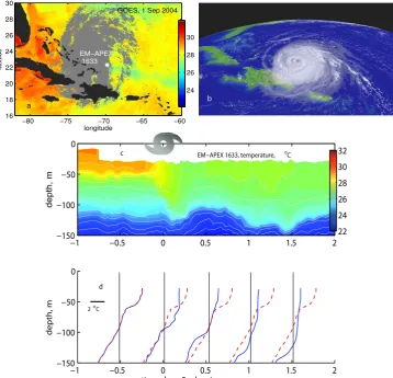
Figure 1: Observations from CBLAST Hurricane Frances (2004) (see Black et al., 2007 for an overview of CBLAST). (a) GOES SST image of the subtropical western North Atlantic and Hur-ricane Frances (clouds are shown as a light gray mass) as it moved west north-west at 5 to 6 m sec−1

over the site where EM-APEX floats had been air-launched one day before; the white asterisk de-notes the position of float 1633 (Sanford et al., 2007). Notice that SST was higher ahead of Hurricane Frances (to the west), than behind. Within the coolest part of the wake, SST was reduced by about 2 to 3◦_{C during the hurricane passage (see also D’Asaro et al., 2007 and Zedler et al., 2009). (b) A nearly}

simultaneous true color image, also from GOES. (c) Time-depth section of temperature measured by EM-APEX float 1633. The color coding of temperature is the same in this section as in the SST map above. The hurricane symbol shows the approximate time during which wind speed exceeded 20 m s−1

. The cloud shield seen in the images above was about twice this size. (d) The corresponding tem-perature profiles. The red dashed profile was observed before the hurricane passage and is repeated as a reference for subsequent profiles that are shown at half-day intervals. The shallowest measured temperature at 30 m depth decreased by about 2.34◦_{C, roughly consistent with the GOES SST image.}

Fig. 1. Observations from CBLAST Hurricane Frances (2004) (see Black et al., 2007 for an overview of CBLAST). (a) GOES SST image of the subtropical western North Atlantic and Hurricane Frances (clouds are shown as a light gray mass) as it moved west north-west at 5

to 6 m s−1over the site where EM-APEX floats had been air-launched one day before; the white asterisk denotes the position of float 1633

(Sanford et al., 2007). Notice that SST was higher ahead of Hurricane Frances (to the west), than behind. Within the coolest part of the

wake, SST was reduced by about 2 to 3◦C during the hurricane passage (see also D’Asaro et al., 2007 and Zedler et al., 2009). (b) A nearly

simultaneous true color image, also from GOES. (c) Time-depth section of temperature measured by EM-APEX float 1633. The color coding of temperature is the same in this section as in the SST map above. The hurricane symbol shows the approximate time during which wind

speed exceeded 20 m s−1. The cloud shield seen in the images above was about twice this size. (d) The corresponding temperature profiles.

The red dashed profile was observed before the hurricane passage and is repeated as a reference for subsequent profiles that are shown at

half-day intervals. The shallowest measured temperature at 30 m depth decreased by about 2.3◦C, roughly consistent with the GOES SST

image.

The emphasis of this paper will be mainly upon ocean models at the other extreme of complexity, in which the same initial ocean data and an understanding of the salient ocean mixing and thermodynamics are combined into a metric (De-Maria et al., 2005),

M(x, y)=F (Ti(x, y, z), ...), (1)

that, with appropriate interpretation, provides forecast guid-ance regarding hurricane-ocean interaction. The functionF, which is the object of this paper, evaluates, integrates or av-erages over depth,z, to yield a two-dimensional, mappable variable, or metric. The ellipsis indicates that more than the

thermal field alone is likely to be relevant. For any specific forecast, a forecast hurricane track is presumed to be avail-able, and thus the relevant position(s) (x, y)are presumed known.

One metric of this sort is the initial sea surface tempera-ture,

SSTi(x, y)=Ti(x, y, z=0). (2)

It is well known that SSTi≥26◦C is a necessary condition for

for hurricane-ocean interaction. It was noted at the begin-ning that SST cools significantly during a hurricane passage. Closely related is that SSTi is likely to be representative of

only the upper few tens of meters of the water column and it is expected that hurricanes will interact with (very roughly) the upper 100 m of the ocean. The physical mechanism(s) of hurricane-ocean interaction and the depth over which inter-action is appreciable are among the central issues for deter-mining an appropriateF.

1.2 Upper Ocean Heat Content, an integral of the ocean temperature

The first ocean metric that took account of the subsurface ocean temperature, called upper Ocean Heat Content (OHC), was written down by Leipper and Volgenau (1972) almost forty years ago

OHC(x, y)=ρoCp

Z 0

Z26

(Ti(x, y, z)−26)dz, (3)

and is today widely used in operational, hurricane forecast-ing (Goni and Trinanes, 2003; DeMaria et al., 2005; and see especially the informative, recent review by Mainelli et al., 2008). The leading factors, ρo=1025 kg m−3 and

Cp=4.0×103J kg−1◦C−1are sea water density and heat

ca-pacity and the lower limit of integration is the depth of the 26◦_{C isotherm, Z}

26. The reference temperature, 26◦C, is an average (dry bulb) temperature in the subtropical atmo-spheric boundary layer and soTi(x, y, z=0)−26 is a

mea-sure of the thermal disequilibrium between the atmosphere and the initial state of the ocean. Aside fromρo andCp,

which are effectively constants, OHC has an obvious inter-pretation as how much (temperature×thickness) ocean tem-perature at a given(x, y)exceeds the reference temperature, 26◦C, and expressed as a heat content. Notice that in the usual case that ocean temperature is monotonically increas-ing toward the surface, water havincreas-ing a temperature less than 26◦C will make no contribution to OHC. A consequence is that OHC can not show how far below the reference temper-ature the ocean tempertemper-ature may be, an issue that arises in Sect. 3.1.2.1

1_{The quantity defined by Eq. (3) has also been called}

hurri-cane heat potential (Leipper and Volgenau, 1972), and tropical cy-clone heat potential (Goni and Trinanes, 2003). To the extent that “heat content” implies conservation properties, these might be bet-ter names (and see Warren (2006) on this common usage of “heat”). Conservation issues are of two kinds, roughly thermodynamic and fluid dynamic. OHC is not conserved under mixing because of changes in density and heat capacity. These errors are very small in the present context, but can be almost completely avoided by use of potential enthalpy (McDougall, 2003). A much bigger conserva-tion error may arise from the lower limit of integraconserva-tion for OHC, the

depth of the 26◦C isotherm,Z26. In the presence of vertical

mix-ing nearZ26, which occurs commonly (Fig. 1b and c, and D’Asaro

et al., 2007), this lower limit is not a material surface whose

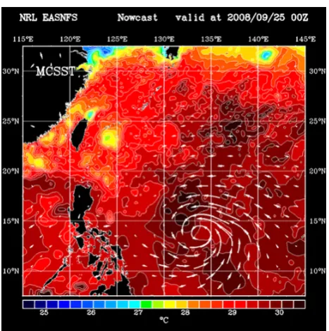
mo-Figure 2: A synoptic map of SST from the East Asian Seas Nowcast and Forecast System (EASNFS) of the Naval Research Laboratory (Ko et al., 2008) for September 25, 2008. The white vectors are low level wind.

excluded from some forecast and analysis schemes (Mainelli et al., 2008). This loss of correlation be-tween hurricane intensity and low range OHC is considered in some detail in Sections 3.1.2 and 3.2.1. 115

The upshot will be that OHC does not bear a consistent relationship to SST in cool, deep ocean

con-ditions or in shallow water and so OHC would not be expected to be a useful metric in those common conditions. To be fair to Leipper and Volgenau (1972), this critique amounts to applying OHC outside of the warm, deep ocean conditions that they envisioned. However, maps of OHC (Goni and Trinanes, 2003) and statistical analyses using OHC as the ocean metric (DeMaria et al., 2005; Mainelli et al., 120

2008) necessarily include all oceanic regions where hurricanes occur, and not excluding regions with small or vanishing OHC. Thus the parameter space of cool SST and shallow water is unavoidable in a discussion of ocean metrics that are intended for more than a qualitative interpretation, the intent here.

7

Fig. 2. A synoptic map of SST from the East Asian Seas Nowcast and Forecast System (EASNFS) of the Naval Research Laboratory (Ko et al., 2008) for 25 September 2008. The white vectors are low level wind.

OHC was not derived from theory so much as it was con-structed ad hoc on the reasonable basis that if hurricane-ocean heat exchange is important to a hurricane, then hurricane-oceanic regions having larger or smaller heat content should be more or less favorable for hurricane formation or intensification (Leipper and Volgenau, 1972; hereafter just intensification). There will be a discussion of mechanisms beginning in Sect. 2, but for now we note that this has been verified, at least in the warm, deep ocean regime (summertime, open Gulf of Mexico) with which Leipper and Volgenau (1972) were most concerned.

tion would be connected by continuity with the surrounding fluid. To appreciate the consequence, imagine that vertical mixing within the ocean surface layer (no hurricane-ocean heat flux) acts to cool

the surface layer, eventually below 26◦C. OHC will vanish as the

surface layer cools below 26◦C and the depthZ26moves upward

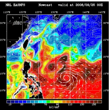
Figure 3: A synoptic map of OHC computed by the EASFNS. The corresponding SST was in the previous figure. Note that the largest values of OHC are found along the axis of the subtropical gyre, roughly 17◦_{N west of Luzon, and especially in mesoscale patches that correspond to relative highs}

of the sea surface height (about 20 cm amplitude). Uniformly low values of OHC are estimated along the northern boundary of this region, and also along the wide, shallow continental shelf south and east of China.

1.3

The goal and the plan of this paper

The object of the present work is a new, rationalized ocean metric for use within a hurricane-ocean forecasting or analysis scheme. The scope is limited to the ocean half of hurricane-ocean interac-tion, and the approach will be to build upon the extensive history of OHC reviewed above, while also making use of 3-d ocean models and guidance from ocean process field studies that were unavailable when OHC was proposed. The starting point is a review of the mechanisms that cause sea surface 130

cooling during a hurricane passage, Section 2.1. This leads to the hypothesis that a verticalaverage of upper ocean temperature is a more relevant metric than is OHC, a vertical integral of ocean temper-ature, Section 2.2. The consequences of averaging (the new metric)vis-a-visintegrating (the present metric, OHC) are explored in Section 3; Section 3.1 considers the deep, open ocean, and Section 3.2 considers a continental shelf. A summary of the present results and remarks on future research are in 135

8

Fig. 3. A synoptic map of OHC computed by the EASFNS. The corresponding SST was in the previous figure. Note that the largest values of OHC are found along the axis of the subtropical gyre,

roughly 17◦N west of Luzon, and especially in mesoscale patches

that correspond to relative highs of the sea surface height (about 20 cm amplitude). Uniformly low values of OHC are estimated along the northern boundary of this region, and also along the wide, shallow continental shelf south and east of China.

OHC takes on the largest values, OHC≥100 kJ cm−2, over oceanic regions having a comparatively warm, thick surface layer, often in association with a subtropical gyre interior or an associated western boundary current system, the Kuroshio or the Gulf of Mexico’s Loop Current (Shay et al., 2000; Halliwell et al., 2008) being important examples. A signifi-cant correlation between these high OHC features and hur-ricane intensification has been found in late summer con-ditions in which the pre-hurricane SST field is often quasi-uniform horizontally (Figs. 2 and 3). Extensive testing and forecasting experience has thus shown that high range OHC, roughly OHC≥60 kJ cm−2_{, provides significant information} on the ocean thermal field beyond that provided by the SSTi

field alone (Goni and Trinanes, 2003; Scharoo et al., 2006; McTaggart-Cowan et al., 2007; Lin et al., 2008; Mainelli et al., 2008; see also Sun et al., 2006).

There are also observations that do not fit comfortably within an OHC framework. At one level anomalies are not surprising; ocean thermal conditions, no matter how they are represented, are not the sole nor necessarily the most impor-tant determinant of hurricane intensity. Large-scale wind and humidity distributions are at least as important, and internal variability occurs within hurricanes on small spatial and time scales that are very difficult to predict (Marks et al., 1998). One notable, apparent anomaly has real consequences for

Figure 4: A map ofT100, the ocean temperature averaged over the upper 100 m or to the ocean bottom (introduced in Section 2.2) computed by the EASNFS of the Naval Research Laboratory. This map was computed on the same ocean temperature field as was OHC of Fig. 3 and may be compared directly. The highest values of OHC andT100corresponding to the subtropical gyre ridge along 15

◦_{N are similar in shape in these maps. The low values are in some respects quite different, especially}

along the southeastern coast of China; OHC indicates low values simply because of shoaling water depth, whereT100indicates fairly high values within a coastal warm boundary layer (defined in Section 3.2.2) that is up to several hundred kilometers in width. This map was kindly provided by Dr. Dong-Shan Ko of the Naval Research Laboratory.

9

Fig. 4. A map ofT₁₀₀, the ocean temperature averaged over the up-per 100 m or to the ocean bottom (introduced in Sect. 2.2) computed by the EASNFS of the Naval Research Laboratory. This map was computed on the same ocean temperature field as was OHC of Fig. 3

and may be compared directly. The highest values of OHC andT₁₀₀

corresponding to the subtropical gyre ridge along 15◦N are similar

in shape in these maps. The low values are in some respects quite different, especially along the southeastern coast of China; OHC in-dicates low values simply because of shoaling water depth, where

T₁₀₀ indicates fairly high values within a coastal warm boundary

layer (defined in Sect. 3.2.2) that is up to several hundred kilome-ters in width. This map was kindly provided by Dr. Dong-Shan Ko of the Naval Research Laboratory.

the parameter space of cool SST and shallow water is un-avoidable in a discussion of ocean metrics that are intended for more than a qualitative interpretation, the intent here. 1.3 The goal and the plan of this paper

The object of the present work is a new, rationalized ocean metric for use within a hurricane-ocean forecasting or anal-ysis scheme. The scope of this paper is limited to the ocean half of hurricane-ocean interaction, and the approach will be to build upon the extensive history of OHC reviewed above, while also making use of 3-D ocean models and guidance from ocean process field studies that were unavailable when OHC was proposed. The starting point is a review of the mechanisms that cause sea surface cooling during a hurri-cane passage, Sect. 2.1. This leads to the hypothesis that a vertical average of upper ocean temperature is a more rel-evant metric than is OHC, a vertical integral of ocean tem-perature, Sect. 2.2. The consequences of averaging vis-a-vis integrating are explored in Sect. 3; Sect. 3.1 considers the deep, open ocean, and Sect. 3.2 considers a continental shelf. A summary of the present results and remarks on future re-search are in the concluding Sect. 4.

2 The oceanic mechanisms of hurricane-ocean interac-tion

Heat content is not a substance that is transferred from the ocean into the atmosphere simply by contact. And specifi-cally, high OHC does not by itself insure that there will be a high heat flux from the ocean into a hurricane. A thermal dis-equilibrium (temperature and humidity difference) between the sea surface and the lower atmosphere must be involved as an intermediary, and all else equal, the larger this disequi-librium, the larger the heat flux. The oceanic part of this is the SST. The route to a new ocean metric begins from this point of view and then requires just three premises. Premise 1, which more or less summarizes the point made just above, is that

P1: The relevant oceanic property for hurricane-ocean interaction is SST and especially the SST underneath a hurricane.

Subsurface ocean temperature (and by extension, OHC) may be very important indirectly, but only to the extent that it ef-fects the SST. The SST underneath a hurricane is singled out in P1 because it corresponds with the high wind speed, cen-tral region of a hurricane and thus the greatest potential for heat exchange (Cione and Uhlhorn, 2003). (P1 seems to elide a role for the other important property of the sea surface, sea state, out of ignorance rather than conviction.) The second premise follows closely on P1.

P2: An oceanic region will be regarded as favor-able for hurricane intensification if the initial SST

is high and if the SST remains high during a hurri-cane passage.

SST should be considered high or low with respect to the at-mosphere just above; absent specific observations, 26◦C is a reasonable reference. Assuming that the initial temperature fieldTi(x, y, z)is given, then the oceanic part of

hurricane-ocean forecasting amounts to predicting the cooling of SST that occurs under a hurricane (taking the hurricane perspec-tive, as is implicit in Fig. 1a) or during a hurricane passage (from the ocean perspective, Fig. 1c).

2.1 Sea surface cooling mechanisms

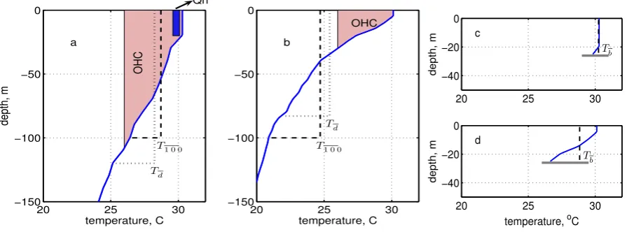
The sea surface underneath a hurricane is cooled by two dis-tinct mechanisms – by hurricane-ocean heat exchange noted above, and by vertical, turbulent mixing of cooler water up-ward into the surface layer (Price, 1981; Jacob et al., 2000; D’Asaro et al., 2007). If the hurricane-induced sea surface cooling noted above was due mainly to heat exchange, then OHC would be an appropriate metric for representing the ocean thermal field. However, two lines of evidence appear to suggest otherwise. Leipper and Volgenau (1972) noted that the large values of OHC found over much of the deep, subtropical oceans are far in excess of the time-integrated heat flux to a given hurricane, often by a factor of 10 or more (noted also by Cione and Uhlhorn, 2003 and by Mainelli et al., 2008). In a later Sect. 3.2, the time-integrated (net) heat flux (sum of latent and sensible fluxes) to a single hurricane is estimated asQnet≈5×107J m−2=5 kJ cm−2(Fig. 5). This net heat flux will cool a water column that is 100 m thick by about only about 0.12◦C, and a 10 m-thick column by about 1.2◦C (Fig. 5). Thus, even a rather shallow, warm continental shelf will have greater heat content, as estimated by OHC, than will be absorbed by a single hurricane. On this basis alone it seems unlikely that OHC per se sets a sig-nificant limit on hurricane-ocean interaction (aside from the case of very shallow water environments). This does not pre-clude that OHC may nevertheless serve as an effective metric for the ocean thermal field in some specific conditions, viz., the warm, deep ocean conditions emphasized by Leipper and Volgenau (1972) (Sect. 3.1.1).

20 25 30 −150

−100 −50 0

temperature, C

depth, m

Qn

OHC

Td

T1 0 0

a

20 25 30

−150 −100 −50 0

temperature, C OHC

Td

T1 0 0

b

20 25 30

−40 −20 0

depth, m

c

Tb

20 25 30

−40 −20 0

temperature, oC

depth, m

d

Tb

Figure 5: Deep, open ocean Argo float temperature profiles from the western, subtropical North

Pa-cific, both of which have SST

≈

30

_{C. These two profiles are rather extreme examples of a deep}

thermocline and a thick surface layer, profile (a) at left, and a shallow thermocline and thin surface

layer, profile (b) at right. OHC is proportional to the lightly shaded area and thus more or less

pro-portional to the thermocline depth. The much smaller, darker shaded area near the surface in (a) is

proportional to an estimate of the net hurricane-ocean heat exchange,

Qn

≈

5

kJ cm

(Section 3.2.2).

The dashed line labeled

T

is the temperature profile after vertical mixing to a depth of 100 m, a

typical depth of mixing by a category 3 hurricane (Section 2.2.1). Note that mixing to 100 m cools

the sea surface of profile (a) by only about 1.5

_{C because the water that was mixed upward into the}

surface layer was only slightly cooler than the water present above

z

= -100 m. Either ocean metric,

OHC or

T

, would indicate that temperature profile (a) is favorable for hurricane intensification. In

profile (b), the cooling effect of the same vertical mixing is much greater,

≈

5

_{C, and notice that}

OHC is also much smaller; both ocean metrics would indicate that profile (b) is not favorable (or

comparatively less favorable) for intensification than is profile (a). The dotted lines labeled

T

are the

temperature profiles after vertical mixing from the surface to a depth of

d

=

120 m (a) or

d

=

85 m (b)

(why these depths is discussed in Section 2.2.2). (c) and (d) The profiles from (a) and (b) but with a

shallow bottom indicated at (arbitrarily) 25 m; discussed in Sections 3.2 and 4.1.

12

Fig. 5. Deep, open ocean Argo float temperature profiles from the western, subtropical North Pacific, both of which have SST≈30◦C. These two profiles are rather extreme examples of a deep thermocline and a thick surface layer, profile (a) at left, and a shallow thermocline and thin surface layer, profile (b) at right. OHC is proportional to the lightly shaded area and thus more or less proportional to the thermocline depth. The much smaller, darker shaded area near the surface in (a) is proportional to an estimate of the net hurricane-ocean heat exchange,

Qn≈5 kJ cm−2(Sect. 3.2.2). The dashed line labeledT₁₀₀is the temperature profile after vertical mixing to a depth of 100 m, a typical depth

of mixing by a category 3 hurricane (Sect. 2.2.1). Note that mixing to 100 m cools the sea surface of profile (a) by only about 1.5◦C because

the water that was mixed upward into the surface layer was only slightly cooler than the water present abovez=−100 m. Either ocean metric,

OHC orT₁₀₀, would indicate that temperature profile (a) is favorable for hurricane intensification. In profile (b), the cooling effect of the

same vertical mixing is much greater,≈5◦C, and notice that OHC is also much smaller; both ocean metrics would indicate that profile (b) is

not favorable (or comparatively less favorable) for intensification than is profile (a). The dotted lines labeledT_dare the temperature profiles

after vertical mixing from the surface to a depth ofd=120 m (a) ord=85 m (b) (why these depths is discussed in Sect. 2.2.2). (c) and (d) The

profiles from (a) and (b) but with a shallow bottom indicated at (arbitrarily) 25 m; discussed in Sects. 3.2 and 4.1.

shows that the net cooling (temperature change times thick-ness) caused by vertical mixing within the upper ocean is ap-proximately equal in magnitude to the net warming caused by vertical mixing in the upper thermocline (this warming is not of direct interest here, but may have relevance over climate time scales, see Sriver and Huber, 2008). Detailed studies of the upper ocean heat budget have found that the ratio of the heat flux due to vertical mixing compared to the hurricane-ocean heat exchange is O(10) in deep water cases (Jacob et al., 2000; Cione and Uhlhorn, 2003; D’Asaro et al., 2007), consistent with the observations noted above. The principle mechanism on the ocean side of hurricane-ocean interaction can then be summarized in Premise 3 – while hurricane-ocean heat exchange may be very important to a hurricane, nevertheless

P3: The large amplitude, 1–4◦C, cooling of the sea surface that occurs during a hurricane passage is due mainly to vertical mixing of cooler water into the ocean surface layer.

2.2 A new ocean metric, depth-averaged temperature

Given P1–P3, it follows that a metric intended to represent the ocean thermal field should account first of all for the sea surface cooling effect of vertical mixing (caused mainly by

the very high winds of a hurricane) and only secondarily for hurricane-ocean heat exchange. Vertical mixing is equiva-lent to vertical averaging, and this leads to the hypothesis advanced in this paper:

H1: The appropriate ocean thermal metric for hurricane-ocean interaction is a vertical average of the initial (pre-hurricane) ocean temperature,

T_d(x, y)= 1 d

Z 0

−d

Ti(x, y, z) dz, (4)

wheredis the depth of vertical mixing caused by a hurricane, i.e., the surface mixed-layer thickness. The depthdhas to be predicted or specified ifT_dis to be pre-dicted, and two methods for doing that are discussed below. If, as will be presumed here,dis evaluated in the wake of a hurricane, then the resulting depth-averaged temperature,T_d, is an estimate of the mixed-layer temperature in the wake.

Given that SST decreases during a hurricane passage, the interpretation of T_d is straightforward. High values ofTd,

values, sayT_d≤24◦_{C, would indicate low values of SST} dur-ing a hurricane passage, and so an ocean thermal field that was comparatively unfavorable (or much less favorable) for intensification.

The dependence of sea surface cooling upon upper ocean stratification is the key property of a depth-averaged temper-ature metric. For example, if there is a comparatively small temperature (vertical) contrast in the water column above z=−dthat is mixed vertically, as in profile (a) of Fig. 5, then vertical mixing will cause comparatively little cooling of the sea surface. If the ocean bottom is shallow and the bottom temperature is warm (Fig. 5c) then, perforce, vertical mixing will cause very little cooling of the sea surface.

The issue now turns to estimation or prediction ofd. At some risk of confusion there are two versions ofdsuggested here. The first is a very simple, empirical, fixed-d version that is based upon the CBLAST field observations of Fig. 1c and Fig. 1d and that serves the most important purpose of this paper – to contrast integrated and averaged ocean tem-peratures. There follows a more complex and more capa-ble variacapa-ble-d version that takes account of the spatially-variable density stratification of the initial ocean and allows for stronger or weaker hurricanes. This variable-d version is better suited for forecasting purposes.

2.2.1 Fixed depth,d=100 m andT₁₀₀

The simplest, plausible version ofd is to take a fixed value, d=100 m, or to the ocean bottom, if that is shallower. The choiced=100 m is admittedly a round number, but is consis-tent with the observed depth of vertical mixing under Hurri-cane Frances (2004) a category 3–4 hurriHurri-cane used here as the base case (by inspection of Fig. 1c and d; see also San-ford et al., 2007 and D’Asaro et al., 2007). The correspond-ing, depth-averaged temperature computed from Eq. (4) is dubbedT₁₀₀(Figs. 4 and 5).

The depth of vertical mixing and the associated SST cool-ing vary significantly in the direction perpendicular to a hur-ricane track; 100 m is the maximum depth of vertical mixing, usually found about 30–70 km to the right of the track of a hurricane moving at a typical speed, 5 m s−1 (Fig. 1a). A mapT₁₀₀(x, y)(Fig. 4) is then the minimum SST expected in a hurricane wake, and not the map for a single hurricane, as in Fig. 1a. The minimum temperature (maximum depth of mixing) was chosen because it is the least ambiguous SST to observe and is the SST that is most frequently cited, e.g., the cooling values of Sect. 1. Whether this depth-averaged tem-perature is the most appropriate SST for hurricane-ocean in-teraction, vs. say the SST under the eye (Cione and Uhlhorn, 2003), is considered on closing in Sect. 4.3.

T₁₀₀has the advantage of great simplicity; it follows from P1, P2 and P3 and the observationd=100 m with no model required. A comparison ofT₁₀₀ with OHC is sufficient to expose the similarities and the differences between a depth-averaged and a depth-integrated temperature, and soT₁₀₀is

emphasized up through Sect. 3.1. However,T₁₀₀ is almost certainly not the best possible depth-averaged temperature for forecasting purposes because mixing to a depth of 100 m is by no means universal. Given an especially stable density stratification (profile b of Fig. 5 or by virtue of a fresh surface layer) or given a minimal hurricane, the depth of mixing may be considerably less.

2.2.2 Variable depthdandT_d

These and other external factors can be accounted by an ocean mixing model that estimates d at each point(x, y). The variable-d metric suggested here requires a good deal more data than does T₁₀₀; the density profile, ρ(z), which will in general require temperature and salinity profiles, as well as a few key pieces of data describing the hurricane of interest. Here we presume Hurricane Frances (2004) (San-ford et al., 2007): radius to maximum winds, Rh (35 km),

translation speed, Uh (5.5 m s−1), and the maximum wind

stress,τ (5.5 Pa). A variable-d metric also requires a param-eterization to connect vertical, turbulent mixing in the upper ocean with the hurricane forcing. The parameterization ap-plied here is that the bulk Richardson number of the surface mixed-layer should not be less than a critical value,C=0.6 (Price, 1981),

g δρ d ρ0(δU )2

≥C or,

g[ρ(z= −d)−−1

d

R−d

0 ρ(z)dz]d ρ0(_ρτ_od4_UR_hhS)2

≥0.6, (5)

wheregis the acceleration of gravity. The operatorδ takes the difference between the surface mixed-layer and the value just below, as if there was a jump in density and velocity. The wind-driven current that appears in the denominator of the Richardson number,δU, has been estimated as the prod-uct of the wind stress-induced acceleration,=τ/ρod, and the

hurricane residence time, 4Rh/Uh. The effects of Earth’s

variable-d metric – omission of all advection, pressure gra-dients and air-sea heat exchange, the specific value ofS – can be checked by comparing the resulting depth-averaged temperature,T_d, against much more comprehensive, 3-D nu-merical ocean model solutions. The comparison is generally favorable, though with some reservations about the lowUh

limit (for details see the Supplementary Material noted at the end of this manuscript).

Given a density profile that is discretized at intervals1z, Eq. (5) can be solved very quickly. The left hand side (lhs) of is evaluated withd=n1zfrom the surface downwards, i.e., withnincreasing from 1. Thelhs starts with very low val-ues, and is a monotonically increasing function ofn (assum-ing that density increases with depth). The equation is con-sidered solved ford whenlhs≥C, or whenn1z=b, where b is the bottom depth and mixing is of course terminated. Once Eq. (5) has been solved ford, the corresponding depth-averaged temperature,T_d, is then estimated by the vertical average, Eq. (4), evaluated over the given initial temperature profile,Ti (from here ond andT_d have this specific

mean-ing). (The Matlab script used to evaluated andT_d on this Argo data is included in the Supplementary Material avail-able online.)

Notice that the denominator of the Richardson number, Eq. 5, depends only upon hurricane parameters that are pre-sumed known and would presumably be fixed for the eval-uation of a given map. The numerator depends only upon the pre-hurricane ocean density profile and will likely vary regionally. The regional variation in a map of T₁₀₀ or T_d (Fig. 4) thus reflects the regional variation of the ocean temperature and salinity (density) field and, where mixing reaches the bottom, the bottom depth.

3 The comparative geography of OHC,T₁₀₀andT_d On first sight, the prescription for a depth-averaged temper-ature via Eq. (4) and the heat content computed via Eq. (3) do not look all that different, and in important and common circumstances (summer, subtropical, deep ocean) they will give essentially the same forecast guidance. In other circum-stances they may be quite different. A corollary of H1 is that a depth-averaged temperature will make a useful ocean met-ric over a much wider range of conditions than does OHC, a depth-integrated temperature. A full test of this important corollary is beyond the scope of this paper. What we can do here usefully is learn where and how OHC and the depth-averaged temperature will differ. To this end, both kinds of metrics have been evaluated using observations from the deep, open ocean (Sect. 3.1) and from an idealized conti-nental shelf (Sect. 3.2). Salinity effects are then noted very briefly in Sect. 3.3.

3.1 The deep ocean

Two open ocean regions were considered; the first was a 20 by 20 degree region of the western subtropical North Pa-cific centered on 20◦N and 130◦E that was studied by Lin et al. (2008). The available Argo temperature and salinity pro-files were acquired for the months July through October of 2007 (846 profiles in total, Fig. 6a). This region spawns some of the largest and most intense hurricanes (super typhoons) found anywhere in the world, and it is also a region having quite pronounced variability of the ocean mesoscale (Qiu, 1999). Eddies having a diameter of several hundred kilo-meters and sea surface height anomalies of±20 cm are com-mon. These mesoscale eddies are accompanied by a raised or depressed thermocline (Fig. 5) and thus by substantial vari-ations of OHC andT₁₀₀that are not reflected in sea surface temperature (Fig. 6b, and compare Figs. 2 and 3 and Figs. 2 and 4). As noted already, Lin et al. (2008) found that the in-tensification of the most intense super typhoons is spatially correlated (coincident) with warm eddies (depressed thermo-cline) that show up as regions of especially high OHC (see Halliwell et al., 2008 for a discussion of mesocale variability in the Gulf of Mexico).

The second open ocean region considered here was the equivalent from the western North Atlantic, 10–30◦N, and 280–320◦and for the same months of 2007. These North At-lantic data (and a few profiles from the Caribbean Sea, 697 profiles total) are almost indistinguishable from the North Pa-cific data, the only difference being fewer points in the range of very large OHC (Fig. 6c and d). Within both data sets there are no doubt many profiles that were significantly ef-fected by a typhoon or a hurricane. There was no attempt to sort these out, and all of the Argo profile data were treated as if they were initial data for the next storm.

15 20 25 30 −200

−150 −100 −50 0

temperature, °C

depth, m

a

N Pacific

20 25 30

18 20 22 24 26 28 30 32

SST, °C T1

0

0

,

◦

C

b

N Pacific

a

b

15 20 25 30

−200 −150 −100 −50 0

temperature, °C

depth, m

c

N Atlantic

20 25 30

18 20 22 24 26 28 30 32

SST, °C d

N Atlantic T1

0

0

,

◦

C

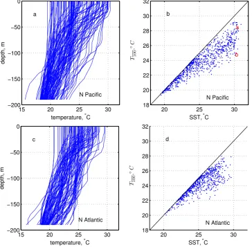
Figure 6: Deep, open ocean Argo float observations used to evaluate the metrics. (a) Argo temperature profiles from the western subtropical North Pacific (every seventh profile of 846 total; salinity not shown). The region sampled was centered on 20◦_{N and 130}◦_{E and included June through October} of 2007. (b) Sea surface temperature (SST; the shallowest measured temperature in a profile) and the depth-averaged temperature,T100, from the profiles at left. Note thatT100and SST are not well correlated, especially in the range of highest SST values. The same is true of SST and OHC and of SST andTd(not shown). The red letters ’a’ and ’b’ denote the (SST,T100) of the profiles of Figs. 5a and b, respectively. (c) Argo temperature profiles from the western subtropical North Atlantic, same time period and 697 profiles in total. (d) SST andT100from the western North Atlantic.

17

Fig. 6. Deep, open ocean Argo float profiles used to evaluate the metrics. (a) Argo temperature profiles from the western subtropical North

Pacific (every seventh profile of 846 total; salinity not shown). The region sampled was centered on 20◦N and 130◦E and included June

through October of 2007. (b) Sea surface temperature (SST; the shallowest measured temperature in an Argo profile) and the depth-averaged

temperature,T100from the same profile. (Note that we might have dubbed the coordinates SSTi, and SSTa, the SST after mixing to 100

m depth.) The distance a point falls below the 1-to-1 line is the cooling caused by mixing to 100 m. The red letters “a” and “b” denote the

(SST,T100) of the profiles of Fig. 5a and b, respectively. (c) Argo temperature profiles from the western subtropical North Atlantic, same

time period and 697 profiles in total. (d) SST andT₁₀₀from the western North Atlantic.

3.1.1 Warm oceans and the high range of OHC

Both of the depth-averaged temperatures are closely related to OHC in the high range of T₁₀₀ , T₁₀₀≥27◦C and OHC, OHC≥75 kJ cm−2_{(Fig. 7b and d). It is not surprising that} an especially warm, thick surface layer will indicate high values of OHC,T₁₀₀ andT_d alike. What is not obvious is that the relationship between high range OHC and highT₁₀₀ appears to be very tight, bijective (one to one), and nearly identical in the western North Pacific and western North At-lantic. Within a given map, the contour lines of highT₁₀₀are essentially parallel with contour lines of high OHC (compare Figs. 3 and 4 over the subtropical gyre). Thus, high values ofT₁₀₀are expected to bear the same qualitative, spatial

cor-relation with hurricane intensification as do high values of OHC (Lin et al., 2008; Shay et al., 2000; Mainelli et al., 2008). A depth-averaged temperature, eitherT₁₀₀orT_d, thus repeats the most useful, demonstrated property of OHC, i.e., high values ofT₁₀₀, roughlyT₁₀₀≥27◦C, will identify open ocean regions where the thermal field is especially favorable for hurricane intensification. This was not accommodated af-ter the fact, but follows straightforwardly from the definition of a depth-averaged temperature, Eq. (4), and the empirical relation between high range OHC andT₁₀₀seen in these data (Fig. 7b and d).

20 22 24 26 28 30 20

22 24 26 28 30

Td,◦C T1

0

0

,

◦

C

a

N Pacific

−50 0 50 100 150

20 22 24 26 28 30

OHC, kJ cm−2 T1

0

0

,

◦C

b

N Pacific

20 22 24 26 28 30

20 22 24 26 28 30

Td,◦C T1

0

0

,

◦

C

c

N Atlantic

−50 0 50 100 150

20 22 24 26 28 30

OHC, kJ cm−2 T1

0

0

,

◦C

d

N Atlantic

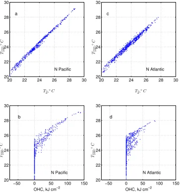
Figure 7: Scatter diagrams of the ocean metrics. (a) The vertically-averaged temperatures,T100 and Td, computed from the Argo profiles of Fig. 6.a (North Pacific). (b) Upper Ocean Heat Content (OHC) andT100for the North Pacific data (and note that this panel is below the corresponding panel (a)). In this deep, open ocean region,T100andTdare highly correlated with each other, and in the higher range of OHC, they are both highly correlated with OHC. In the low range of OHC, where SST is close to 26◦_{C, the correlation between OHC and the depth-averaged temperatures is poor. OHC} is zero on profiles where the temperature is less than 26◦_{C throughout the water column, about one} third of the profiles in this sample. (c) The vertically-averaged temperatures,T100andTd, computed from the North Atlantic Argo profiles Fig. 6c. (d) OHC andT100from the North Atlantic data of (c). Same comments as apply for the North Pacific data.

19

Fig. 7. Scatter diagrams of the ocean metrics. (a) The vertically-averaged temperatures,T₁₀₀andT_d, computed from the Argo profiles of

Fig. 6a (North Pacific). (b) Upper Ocean Heat Content (OHC) andT₁₀₀ for the North Pacific data (and note that this panel is below the

corresponding panel (a)). In this deep, open ocean region,T₁₀₀ andT_dare highly correlated with each other, and in the higher range of

OHC, they are both highly correlated with OHC. In the low range of OHC, where SST is close to 26◦C, the correlation between OHC and

the depth-averaged temperatures is poor. OHC is zero on profiles where the temperature is less than 26◦C throughout the water column,

about one third of the profiles in this sample. (c) The vertically-averaged temperatures,T₁₀₀andT_d, computed from the North Atlantic Argo

profiles Fig. 6c. (d) OHC andT₁₀₀from the North Atlantic data of (c). Same comments as apply for the North Pacific data.

continue on (though in light of P1 and P2 we might still ask why there is a correlation between high OHC and hurricane intensification). As discussed in Sect. 3.2, there may be shal-low water regions that are equally favorable for hurricane intensification as assessed by a depth-averaged temperature, and yet that have comparatively low OHC. Cool, deep ocean regions are also relevant and interesting.

3.1.2 Cooler oceans and the low range of OHC

thermal metric would be expected to have a low range within which hurricane intensity is damped.

A partial resolution of this low OHC puzzle may be as close at hand as P1 and Eq. (3). And specifically, the loss of the tight relationship between high range OHC and the depth-averaged temperatures results in part from a slightly peculiar property built into OHC, i.e., that all ocean temper-atures less than the reference temperature 26◦C are treated the same, effectively as zero. For example, if the tempera-ture of the entire water column was 0◦C, then the estimated OHC would be zero, and if the temperature of the entire wa-ter column was 26◦C, then the OHC would again be exactly zero. Thus, insofar as OHC is concerned,T=0 andT=26◦C are one and the same. As a consequence, roughly a third of the open ocean temperature profiles considered here (Fig. 7) map into one point in OHC-space, OHC=0, which might be termed a cool degeneracy. In maps of OHC, this cool de-generacy appears as broad regions that are at or near zero and so horizontally uniform. There is just a hint of this cool degeneracy along the northern boundary of the North Pa-cific OHC map computed in late September (Fig. 3) and it becomes quite prominent once seasonal cooling has devel-oped in late October (see Goni and Trinanes (2003) and http: //www.aoml.noaa.gov/phod/cyclone/data/go.html for exam-ples).

In Sect. 1 it was noted that the reference temperature of OHC, 26◦C, had a significant empirical basis. But whether there is a literal cutoff in hurricane-ocean interaction for SST≤26◦C as occurs with OHC seems unlikely, if only be-cause the dew point temperature of the hurricane lower at-mosphere is typically a few ◦_{C less than the air} tempera-ture, and so some latent heat flux would be expected even for SST≤26◦C. What appears to be certain is that OHC de-fined by Eq. (3) will have poor (or no) resolution in regions where the upper ocean temperature is less than 26◦C and hence OHC could not be expected to provide a nuanced ac-count of the possible damping effect of still lower SST. This limitation of OHC is not shared by a depth-averaged tem-perature, which can always be referenced to 24 or 26◦C. For example, maps ofT₁₀₀−26 or (Ti+T100)/2−26 (discussed in Sect. 4.3) would give a much more vivid impression of a warm or cool sea surface than doesT₁₀₀alone.

3.2 The coastal ocean

OHC and the depth-averaged temperatures can be quite dif-ferent when evaluated over shallow water regions. The con-sequence for forecasts of hurricane-ocean interaction may be more or less significant depending upon the extent of the shallow water area affected and the relationship of a hurri-cane track to the coastline (incidence angle). The shallow water limit is of interest in the present context because it clearly shows the difference between integrating and aver-aging. The shallow water limit is of considerable practical

importance for hurricane forecasting since it occurs in con-junction with hurricane land fall.

To illustrate the effects of bottom depth, OHC andT_dwere evaluated over an idealized continental shelf that was con-structed along the lines of the West Florida Continental Shelf (Fig. 8a). The bottom slope was taken to be∂b/∂x=10−3 and constant, with b the bottom depth, and x the across-shelf coordinate. The hydrography of continental shelves varies a great deal from region to region and on a given shelf with time (Allen et al., 1983) with important conse-quences for what follows. But given that the goal here is to illustrate bottom depth effects alone, the thermocline was presumed to be level so thatTi(x, y, z)=Ti(z)and

hor-izontally homogeneous for z≥−b(x). i.e., upwelling neu-tral. The temperature profileTi(z)was taken from the West

Florida Shelf in summer (Hu and Muller-Karger, 2007) and had a warm and quasi-uniform surface layer about 25 m thick, and a comparatively large vertical gradient of tem-perature, 0.15◦C m−1, within the seasonal thermocline. This kind of shallow, strongly stable seasonal thermocline is typ-ical of subtroptyp-ical shelf regions that are not directly influ-enced by deep ocean currents, e.g., the South and Middle Atlantic Bights (Schofield et al., 2008), if not impacted by Gulf Stream-derived eddies, or the shelf regions along the northern Gulf of Mexico, aside from Loop Current eddies. The metrics OHC andT_dwere then sampled along a transect across the shelf (Fig. 8b and c).

3.2.1 Coastal ocean OHC

To evaluate OHC over shallow waters in which the bottom temperature exceeds 26◦_{C, the lower limit of integration was} presumed to be the bottom depth,b. Given this specific shelf and hydrography, the estimated OHC begins to decrease as the bottom depth becomes less than the depth of the 26◦C isotherm, which is about 50 m in the temperature profile pre-sumed here (Fig. 8b). Assuming a consistent deep-ocean and coastal-ocean interpretation of OHC, i.e., that regions having OHC≤50 kJ cm−2are not favorable for hurricane intensifi-cation (or at least less so than high OHC regions), then ac-cording to OHC, a shallow continental shelf would appear to be an unfavorable environment for hurricane intensification.

0 20 40 60 80 100 120 −120

−100 −80 −60 −40 −20 0

depth, m

a Temperature(z)

0 20 40 60 80 100 120 0

20 40 60 80

OHC, kJ cm

−2

b Ocean Heat Content

0 20 40 60 80 100 120 24

26 28 30

Td

,

◦

C

distance offshore, km; bottom depth, m c

ICCL

CWL

Td

Td−Qnet/ρC pb

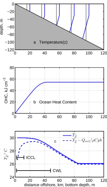
Fig. 8. The variation of OHC andT_dalong a transect of an ide-alized continental shelf that could be characterized as fairly broad and upwelling neutral. (a) The temperature profile came from the

West Florida Continental Shelf. The thin vertical lines are at 26◦C

and the scale for temperature is as for distance. The bottom slope is about 1.5 to 2 times that of the West Florida Shelf. (b) OHC

decreases with decreasing bottom depth,d≤40 m, which is slightly

less than the depth of the 26◦C isotherm. (c) SST profiles across the

shelf. The SST_i(not shown) was taken to be 30◦C and uniform.T_d

increases with decreasing bottom depth less than 85 m, the depth of mixing estimated for this stratification over a deep ocean. The

dashed line isT_dmodified with a nominal heat loss to the hurricane.

ICCL is the width of the Inner-Coastal Cool Layer (Sect. 3.3.2) and CWL is the width of the Coastal Warm Layer.

OHC over the deep ocean. The combined effect of this cool and shallow water degeneracy is thought to be a part of the reason that OHC does not show a correlation with hurricane intensification in the low range of OHC.

3.2.2 Coastal oceanT_d

A coastal warm layer. Given the shelf topography and strat-ification presumed here, the depth-averaged temperatureT_d increases as the bottom depth becomes less thanddo=85 m,

the depth of mixing over the deep ocean given this rather sta-ble stratification. The increase ofT_d shoreward of the 85 m

isobath (Fig. 8c) follows from the increase of bottom tem-perature with decreasing bottom depth, i.e., there is less cold water available to be mixed upwards. This can be expected over a shelf on which the seasonal thermocline intersects the bottom, i.e., over shelves that are either upwelling neutral or negative, but not on shelves that are upwelling positive. The end result for an upwelling neutral shelf is that the across-shelf temperature profileT (x)exhibits what might be termed a Coastal Warm boundary Layer (CWL), whose half-width may be estimated roughly as

WCW L≈

1 2ddo/

∂b

∂x, (6)

and in this case,WCW L=42 km.

An inner-coastal cool layer. Heat loss to the hurricane must become a significant process for sea surface cooling where the water is shallow enough (Shen and Ginis, 2003). To account approximately for this hurricane-ocean heat ex-change, the depth-averaged temperatureT_dcan be perturbed by subtracting a typical net hurricane-ocean heat flux,Qnet, from the water column. Qnetis estimated from the numer-ical simulation of the Frances (2004) case by Sanford et al. (2007) by integrating the latent and sensible heat fluxes over a period of one day centered on the hurricane passage, Qnet≈5×107J m−2, or in the non-SI units often used for OHC,Qnet≈5 kJ cm−2. This estimate appears to be at least roughly consistent with the heat fluxes estimated by Chen et al. (2007) for the Frances (2004) case, and by Cione and Uhlhorn (2003) for other hurricanes. The revised depth-averaged temperature that takes account of this heat loss, T_d−Qnet/ρoCpb, where b is the water depth, is shown as

the dashed line of Fig. 8c. The resulting Inner-Coastal Cool boundary Layer (ICCL), follows the qualitative expectations of OHC in the sense that the cooling is inversely related to water depth,b. The width of this cool layer may be estimated roughly as the region where the temperature is decreased by say1T=1◦C or more,

WICCL≈ Qnet ρoCp1T

/∂b

∂x, (7)

and in this case,WICCL=12 km.

is considerably wider than the inner cool layer. For typical bottom slopes and heat loss values,

WCWL WICCL

= ddo/2 Qnet/ρoCp1T

≈3.5 (8)

3.2.3 Applications and coastal ocean observations

The maps of Figs. 3 and 4 showT₁₀₀ and OHC evaluated over the broad, shallow continental shelf off of the south and east coast of China (South China Sea north to the Yellow Sea). These are depicted as regions of generally low OHC, ≤40 kJ cm−2, despite having fairly high SST, simply because they are shallow. In contrast, the estimated depth-averaged temperature (Fig. 4 isT₁₀₀which has the same relation to bot-tom depth as doesT_d) indicates that these shelf regions are likely to remain fairly warm during a hurricane passage by virtue of the CWL phenomenon. Hence on our P3 (Sect. 2.1) these shelf regions appear to be somewhat favorable for hur-ricane intensification, as seen in a depth-averaged tempera-ture T₁₀₀≥27◦C. Some of the effected shelf regions are as wide as several hundred kilometers and likely to be of signif-icance for hurricane-ocean interaction, or at least for our pre-diction of hurricane-ocean interaction. Other shelf regions appear nearly the same when diagnosed with OHC orT₁₀₀, notably east of the Phillipines, where the continental shelf is quite narrow. To summarize, the distribution ofT₁₀₀ in-dicates that some coastal oceans – those having broad, shal-low continental shelves and hydrography that is upwelling neutral or negative – are expected to remain warm during a hurricane passage, and in that regard would appear to be fa-vorable environments for hurricane intensification. This is a result at odds with a consistent deep-ocean/shallow-water interpretation of OHC.

As hurricanes cross a continental shelf they are also likely to be making land fall, which is usually expected to cause a rapid and significant decrease of hurricane intensity (but see McTaggart-Cowen et al. (2007) who note that this is not necessarily the case if the land surface is flat, warm and wet, e.g., South Florida). However, our concern here is exclu-sively with the ocean thermal field, and some evidence is that shallow water environments may indeed be favorable for hur-ricane intensification in the sense that hurhur-ricane-induced sea surface cooling has been observed to be reduced over shallow water regions compared to the cooling over outlying, deep water regions. Hazelworth (1968) analyzed the time series data from weather ships for hurricane passages and made a very brief and tentative mention of such a shallow water ef-fect. The first explicit report was evidently made by Cornil-lon et al. (1987), and more recently this phenomenon has been observed on the West Florida Continental Shelf by Hu and Muller-Karger (2003). The latter two studies inferred that the principal cause of the reduced sea surface cooling over shallow water was the absence of cool water at depths that could be mixed into the surface layer, just as happens here with the depth-averaged temperature. Emanuel (1999)

noted the relevance of this shallow water effect in the context of hurricane-ocean interaction.2

3.3 Salt-stratified water column

In the event that salinity makes an important contribution to the upper ocean density stratification, thenT_d can, in prin-ciple, differ from both OHC and T₁₀₀ which acknowledge temperature only. Important salinity effects may arise where there is a comparatively fresh ocean surface layer, which of-ten occurs in a coastal ocean, and especially down-coast from the estuary of a major river (Bingham, 2007). There are also open ocean regions in which salinity makes an appreciable contribution to the static stability of the upper ocean, e.g., the barrier layer of the western tropical Pacific and parts of the northern Indian Ocean (McPhaden et al., 2009).

If the net salinity anomaly (thickness times salinity anomaly in the initial state) is as large as about 20 m, then the fresh layer will inhibit vertical mixing significantly. The effect upon the sea surface temperature will depend upon whether the fresh layer is warmer or cooler than the water below. If the former, then salinity stratification will act to re-duce the depth of vertical mixing and thus sea surface cool-ing. If the latter, then vertical mixing will act to increase the surface temperature (see the Nordic Sea example of Saetra et al., 2003), a possibility missing altogether from OHC, which omits any reference to salinity (or density). This anomalous surface warming effect of vertical mixing is present inT₁₀₀ when the temperature profile has an inversion, but in gen-eral, a salinity effect upon static stability requires an explicit treatment of density, e.g., by means ofT_dor something more comprehensive.

4 Closing remarks

4.1 Summary

The standard metric of the ocean thermal field within hurricane-ocean interaction is a depth-integrated ocean tem-perature, upper Ocean Heat Content or OHC. OHC has been shown to provide valuable forecast guidance in warm, deep ocean conditions for which it was first formulated (Leipper

2_{During the summer of 2005 there were a number of intense}

and Volgenau, 1972; Lin et al., 2008; Mainelli et al., 2008) but the argument made here is that a depth-averaged tem-perature,T₁₀₀ orT_d, may be more appropriate over a much wider range of conditions. The argument was made on three premises: P1, that SST and especially SST under a hurri-cane is the directly relevant ocean variable; P2 an ocean re-gion is favorable for hurricane intensification if SST remains high during a hurricane passage; and P3, the observation that cooling is due mainly to vertical mixing rather than to hurricane-ocean heat exchange. The hypotheses of this pa-per follows: H1 a depth-averaged ocean tempa-perature is the appropriate metric (or proxy) for SST under a hurricane, and the corollary is that a depth-averaged temperature is a more robust metric of hurricane-ocean interaction than is OHC.

The majority of hurricanes and typhoons form over the deep, open ocean in late summer when sea surface tempera-ture is warmest. In that most important circumstance, OHC and T₁₀₀ or T_d will provide essentially the same forecast guidance, i.e., that an ocean region having a warm (T≥26◦_C) and especially thick surface layer will be a favorable environ-ment for hurricane intensification. This has been observed to hold in forecasting practice (Sect. 1.2). This observation could be taken as a warrant for the original rationale for OHC – that a high OHC region resists cooling due to hurricane-ocean heat exchange. This is true, of course, but we have argued in Sect. 2.1 that it is not highly germane. Equally, this observation could be taken as evidence in favor ofT₁₀₀ orT_d– that a thick, warm surface layer resists the cooling ef-fect of vertical mixing. This latter interpretation is espoused in most recent studies (Lin et al., 2008; McTaggart-Cowen et al., 2007; Mainelli et al., 2008) and is the interpretation that is consistent with a depth-averaged temperature met-ric. If only warm and deep ocean conditions were relevant to hurricane-ocean interaction, then this inference of mech-anisms would be of academic interest, but would hold little practical importance (Fig. 9).3

3_{The seasonal cycle of cooling on warm subtropical}

continen-tal shelves serves as an interesting counterpoint to the hurricane-ocean interaction phenomenon of interest here. Around the Gulf of Mexico, the cooling phase of the seasonal cycle begins in earnest with the first cold air outbreak (see the satellite imagery noted above and the cold air outbreak beginning in mid-October, 2005 following the passage of Hurricane Wilma, 2005). Where a hurricane can be characterized by very strong winds and a rather small air-sea tem-perature difference, cold air outbreaks over the Gulf of Mexico are the complement in the sense that they have moderate wind speeds but very cold and dry air that sets up a very large air-sea temper-ature difference that is sustained for several days. Hence, while a cold air outbreak must cause some vertical mixing (Lentz et al., 2003), it will certainly also cause very significant heat loss from the ocean. The spatial pattern of the sea surface cooling follow-ing a cold air outbreak follows the qualitative expectations of OHC: shallow, inner shelf regions (small OHC) clearly cool in advance of deeper, outer shelf regions (larger OHC). The cooling phase of the seasonal cycle on subtropical continental shelves might thus be

However, there are three other fairly common circum-stances in which the inference of mechanism is crucially im-portant in as much as OHC and depth-averaged temperature will give quite different forecast guidance.

Cool, open ocean waters. Hurricanes form over warm (SST≥26◦_{C) ocean regions, but may later move over much} lower SSTs during their lifetime (a striking example is shown by Monaldo et al., 1997). The cool degeneracy built in to OHC effectively restricts its application to warm ocean con-ditions. The depth-averaged temperatures do not have this property, and an analysis ofT₁₀₀ or T_d could, in principle, permit the forecast of a damping effect of cool sea surface temperatures upon hurricane intensity.

Salt-stratified waters. While temperature is a sufficient proxy for density and static stability in most conditions, salinity can have a significant and sometimes decisive effect on static stability in special locations, for example within or near estuaries. OHC andT₁₀₀ are silent on salinity effects, which can be accounted by theT_d metric provided that the initial salinity is known.

Shallow waters. OHC and the depth-averaged temperatures can be quite different when evaluated over shallow, continen-tal shelf regions. OHC will generally indicate that shallow re-gions (shallow compared to the depth of the 26◦C isotherm) are an unfavorable environment for hurricane intensification, whileT₁₀₀orT_dmay indicate the opposite, that shallow re-gions (shallow compared to the depth of vertical mixing in the deep ocean) can be favorable for hurricane intensifica-tion compared to an otherwise similar deep ocean (Fig. 9). To the point – this study indicates that, land effects aside, a shallow, warm continental shelf may be as favorable for hur-ricane intensification as is a deep, open ocean, warm regime, e.g., the Loop Current or warm eddies of the subtropical gyre interior (compare the depth averaged-profiles of Fig. 5a and c).

4.2 Remarks on the coastal ocean

The variation of SST with distance offshore is at once the most readily observed property of the coastal ocean and is the property of immediate interest for hurricane-ocean in-teraction and forecasting. It is important to appreciate that the specific relationship between SST and distance offshore shown in Fig. 8c is by no means universal because the hy-drography of any given continental shelf may be quite differ-ent from the upwelling neutral case considered in Sect. 3.2. The thermal field on most continental shelves depends upon the depth and (at least) the cross-shelf coordinate,x, so that T=T (x, z). In shelf regions that are upwelling positive, e.g., Campeche Bank or the Louisiana-Texas shelf in late summer

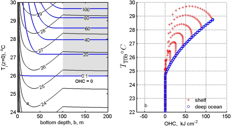
Fig. 9. (a) Dependence of OHC (thin dark blue lines) andT₁₀₀(thicker gray lines) upon initial ocean temperature and bottom depth. The

bottom slope was as in Fig. 8a. The temperature profile had a 30 m thick mixed layer and a constant vertical gradient, 0.05◦C m−1, typical

of the open ocean. The temperature was varied by subtracting a constant, 0 to 6◦C, from the entire profile. Both OHC andT₁₀₀increase with

increasing ocean temperature. Over the deep ocean and for warm temperatures, OHC andT₁₀₀are similar (the lightly shaded, upper right

quadrant). However, the dependence upon bottom depth is quite different and reflects the difference between vertically-integrating, OHC,

which has a maximum at the warmest temperature and the greatest bottom depth, or vertically-averaging,T₁₀₀, which has a maximum at the

warmest temperature and a bottom depth of 30 m, the initial mixed layer thickness. (b) A scatter diagram of the data at left. The big blue dots are from the deep ocean, and the fan of red points are from the continental shelf (the spacing of these points is arbitrary). Notice that for

this temperature profile (constant vertical gradient) OHC andT₁₀₀are exactly similar for warm temperatures over the deep ocean (cf. Fig. 7b

and d where this is not the case). OHC andT₁₀₀are decidedly not similar over the continental shelf.

(Walker, 2005; see also the SST imagery of the Supplemen-tary Material), the thermocline will be lifted toward the coast (∂T_∂x≥0 for the configuration of Fig. 8a) so that cool water may be present very close to shore and very close to the sea surface. Over such an upwelling positive shelf region there may be greater SST cooling than over the outlying, deep ocean, i.e., the reverse of the CWL phenomenon. On some shelves, e.g., the Middle Atlantic Bight, the early sum-mer thermocline may be thin enough, O(30 m) (Schofield et al., 2008) that the width of the coastal warm layer may be no more than a few kilometers, and negligible. Given the great range and temporal variability of coastal ocean hydrography, a key requirement for forecasting hurricane-ocean interaction over shelf regions will be to observe and to model the ocean stratification in more or less real time.

The present treatment of the coastal ocean response to a hurricane (Sect. 3.2.2) was simplified to the point that T_d could be characterized as a null model: the estimated (deep ocean) vertical mixing was simply stopped if it reached the ocean bottom. That must happen, of course, but so may a great deal else that was outside the scope of this greatly sim-plified treatment. For example, rotary inertial motions, the dominate mode of open ocean, wind-driven currents, must be

22

23

24

24

24

25

25

25

26

26

26

27

27 27

28

28 28

29

29

(T1 0 0+ Ti(z = 0))/2,

o C

T i

(z=0),

o C

bottom depth, b, m

0 50 100 150 200

24 25 26 27 28 29 30

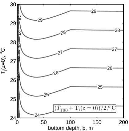
Fig. 10. The simple average ofT₁₀₀and the initial SST for the data of Fig. 9a. This temperature is thought to be a better estimator of the SST under the high wind speed, central region of a hurricane than

isT₁₀₀, and in that regard may be the most relevant SST insofar as

hurricane-ocean interaction is concerned. It is, of course, also much harder to observe. Notice that this temperature is slightly greater

thanT₁₀₀over the deep ocean,z>−b(cf. Fig 9a) and nearly equal

toTiover the mid-continental shelf.

4.3 A look ahead

Forecasting of hurricanes or any natural phenomenon is a pragmatic endeavor. Insight from models and observations can help point the way to new hypotheses or methods, but forecasting success can only be told from actual practice (Lin et al., 2008; Mainelli et al., 2008) which was beyond the scope of this paper. The best result of this discussion would be to stimulate a fresh look at hurricane-ocean inter-action, and specifically, to encourage further testing of ocean metrics drawn from an expanded hypothesis-space. Just two examples:

A revised OHC. The conservation error of OHC (footnote 1 of Sect. 1)and the cool degeneracy noted in Sect. 3.1.2 could be remedied for most hurricane analysis or forecasting pur-poses simply by choosing a reference temperature that is be-low the depth of vertical mixing and the be-lower limit of rel-evant SSTs, e.g., 22◦_{C. This variant of OHC will have} im-proved conservation and statistical properties over a wider range of conditions than does the usual form, Eq. (3), but there is still no guarantee that heat content will be the most relevant physical quantity for hurricane-ocean interaction over shallow continental shelves (Sect. 3.2) and especially those that are to some degree salt-stratified (Sect. 3.3). A derivative of T_d. The depth-averaged temperatures es-timated here were intended to be the minimum of SST

expected in a hurricane wake, i.e., displaced behind the strongest winds of a moving hurricane. The SST cooling di-rectly under a hurricane can be considerably less than the maximum cooling seen in the wake (Cione and Uhlhorn, 2003; D’Asaro et al., 2007, and see also Wu et al., 2005), and it seems likely that hurricane-ocean interaction would be better represented by, e.g., a weighted average of the ob-served, initial SST andT_d (a simple average is in Fig. 10). In a similar way, if the issue on a given day was the possi-ble intensification of a moderate tropical storm, then a much reduced wind stress amplitude in the mixing depth model (Eq. 5),τ=1 Pa, would be appropriate. Treatment of very slowly moving or quasi-stationary storms would benefit from an explicit treatment of upwelling (see the remarks in the Supplementary Material) and, in shallow water, heat loss to the hurricane.

Identifying the optimum ocean metric is an important and significant challenge; OHC and depth-averaged temperatures are well-correlated in some important circumstances and, in any event, the ocean thermal field is just one of several fac-tors that make up the complex environment of a hurricane. A thorough exploration and sensitive test of ocean metrics will require a large suite of case studies that span the full range of ocean conditions that are relevant for hurricane-ocean inter-action. No doubt such a study could be aided considerably by guidance from the best possible air and sea coupled models that include a coastal ocean.

Supplementary Material

Supplementary material includes:

1. A Matlab script that evaluates an arbitrary density pro-file for the depth of mixing and the depth-averaged tem-perature,Td.

2. A description of a comparison ofTd with solutions of

the 3D-PWP numerical ocean model.

3. A collection of GOES SST imagery of the Gulf of Mex-ico during the summer of 2005.

Available online:

http://www.ocean-sci.net/5/351/2009/ os-5-351-2009-supplement.zip

Acknowledgements. This research was supported by the US