Atmos. Meas. Tech., 6, 419–429, 2013 www.atmos-meas-tech.net/6/419/2013/ doi:10.5194/amt-6-419-2013
© Author(s) 2013. CC Attribution 3.0 License.
EGU Journal Logos (RGB)
Advances in
Geosciences
Open Access
Natural Hazards
and Earth System
Sciences
Open AccessAnnales
Geophysicae
Open AccessNonlinear Processes
in Geophysics
Open AccessAtmospheric
Chemistry
and Physics
Open AccessAtmospheric
Chemistry
and Physics
Open Access DiscussionsAtmospheric
Measurement
Techniques
Open AccessAtmospheric
Measurement
Techniques
Open Access DiscussionsBiogeosciences
Open Access Open Access
Biogeosciences
DiscussionsClimate
of the Past
Open Access Open Access
Climate
of the Past
Discussions
Earth System
Dynamics
Open Access Open Access
Earth System
Dynamics
DiscussionsGeoscientific
Instrumentation
Methods and
Data Systems
Open Access
Geoscientific
Instrumentation
Methods and
Data Systems
Open Access DiscussionsGeoscientific
Model Development
Open Access Open Access
Geoscientific
Model Development
DiscussionsHydrology and
Earth System
Sciences
Open AccessHydrology and
Earth System
Sciences
Open Access DiscussionsOcean Science
Open Access Open Access
Ocean Science
DiscussionsSolid Earth
Open Access Open Access
Solid Earth
Discussions
The Cryosphere
Open Access Open Access
The Cryosphere
Discussions
Natural Hazards
and Earth System
Sciences
Open Access
Discussions
Position error in profiles retrieved from MIPAS observations with a
1-D algorithm
M. Carlotti1, E. Arnone2, E. Castelli2, B. M. Dinelli2, and E. Papandrea1
1Dipartimento di Chimica Fisica e Inorganica, University of Bologna, Viale Risorgimento 4, 40136 Bologna, Italy 2ISAC – CNR, Via P. Gobetti 101, 40129 Bologna, Italy
Correspondence to: M. Carlotti ([email protected])
Received: 18 May 2012 – Published in Atmos. Meas. Tech. Discuss.: 12 September 2012 Revised: 28 January 2013 – Accepted: 28 January 2013 – Published: 20 February 2013
Abstract. The information load (IL) analysis, first intro-duced for the two-dimensional approach (Carlotti and Mag-nani, 2009), is applied to the inversion of MIPAS (Michel-son Interferometer for Passive Atmospheric Sounding) ob-servations operated with a 1-dimensional (1-D) retrieval al-gorithm. The IL distribution of MIPAS spectra is shown to be often asymmetrical with respect to the tangent points of the observations and permits us to define the preferential latitude where the profiles retrieved with a 1-D algorithm should be geo-located. Therefore, defining the geo-location of the re-trieved profile by means of the tangent points leads to a “po-sition error”. We assess the amplitude of the po“po-sition error for some of the MIPAS main products and we show that the IL analysis can also be used as a tool for the selection of spectral intervals that, when analyzed, minimize the position error of the retrieved profile. When the temperature (T) pro-files are used for the retrieval of volume mixing ratio (VMR) of atmospheric constituents, theT-position error (of the or-der of 1.5 degrees of latitude) induces a VMR error that is directly connected with the horizontalT gradients. Temper-ature profiles can be externally-provided or determined in a previous step of the retrieval process. In the first case, the IL analysis shows that a meaningful fraction (often exceeding 50 %) of the VMR error deriving from the 1-D approxima-tion is to be attributed to the mismatch between the posiapproxima-tion assigned to the externalT profile and the positions whereT is required by the analyzed observations. In the second case the retrievedT values suffer by an error of 1.5–2 K due to neglecting the horizontal variability ofT; however the error induced on VMRs is of minor concern because of the gener-ally small mismatch between the IL distribution of the obser-vations analyzed to retrieveT and those analyzed to retrieve
the VMR target. An estimate of the contribution of theT -position error to the error budget is provided for MIPAS main products. This study shows that the information load analy-sis can be successfully exploited in a 1-D context that makes the assumption of horizontal homogeneity of the analyzed portion of atmosphere. The analysis that we propose can be extended to the 1-D inversion of other limb-sounding exper-iments.
1 Introduction
atmosphere increases, by effect of the satellite movement, up to a length of about 2000 km making therefore the hor-izontal homogeneity assumption a weak point of the analy-sis. A two-dimensional (2-D) tomographic approach, named geo-fit (Carlotti et al., 2001), was introduced for the MIPAS (Michelson Interferometer for Passive Atmospheric Sound-ing) experiment in order to overcome the horizontal homo-geneity assumption; it can be used for any limb-scanning satellite experiment where the lines of sight of the spectrom-eter are oriented (and overlap) along the orbit track. With geo-fit the horizontal inhomogeneities are modelled and re-trieved through the simultaneous analysis of observations be-longing to all the limb-scans measured along a whole orbit. Other 2-D retrieval algorithms (e.g. Livesey and Read, 2000; Steck et al., 2005; Puk¸¯ıte et al., 2008), exploit 2-D strategies. However, despite of the demonstrated advantages of the 2-D approach, orbiting limb-scanning experiments are mostly analyzed using 1-D algorithms.
In 1-D analyses the geo-location assigned to the retrieved profiles is generally connected with the position of the tan-gent points of the observations. A common choice is to geo-locate the whole profile at the average geographical coordi-nates of the tangent points of the analyzed scan. The size of the possible geo-location error qualifies the retrieval products but it is not considered to be of concern within the retrieval process because, thanks to the horizontal homogeneity as-sumption, the profile position is not relevant within the por-tion of atmosphere spanned by the observapor-tions. However, the profile geo-location becomes relevant when it is used to identify coincidence with independent measurements or to calculate average distributions within predefined latitudinal bands (Kiefer et al., 2010).
The inversion of limb-scanning observations usually re-quires the knowledge of temperature (T) profiles for the re-trieval of any atmospheric constituent. The quality ofT pro-files used in volume mixing ratio (VMR) retrievals is then crucial since their error propagates into the error of the re-trieved VMR values. It is therefore necessary to provide an estimate of the errors introduced by 1-D algorithms as a con-sequence of neglecting the horizontalT gradients. In a VMR retrieval theT profile can be externally-provided or deter-mined in a previous step of the retrieval analysis. In the first case, the external profile is chosen trying to mach at best the time and geo-location of the analyzed observations but an error is expected as a consequence of possible mismatches. In the second case perfect coincidence is achieved (since the profile has been obtained from the same observations) but T profiles retrieved by neglecting horizontal gradients are known to be affected by a systematic error due to the hor-izontal homogeneity assumption.
In order to analyze the nature and the size of the errors in-volved in the scenarios described in the previous paragraph, we have studied the 1-D inversion of MIPAS observations. For the purpose we have exploited, within the 1-D context, the information load (IL) analysis (Carlotti and Magnani,
2009) first introduced to study the information contained in consecutive limb-scanning observations when they are ana-lyzed with a 2-D approach (a sample application of IL anal-ysis for 2-D retrievals can be found in Carlotti et al. (2011)). Retrievals on simulated observations have been used to quan-tify the errors introduced by 1-D algorithms as a consequence of neglecting the horizontal gradients.
This paper is organized as follows: in Sect. 2 we briefly de-scribe the features of the MIPAS experiment that are relevant for this study, and the 1-D retrieval algorithm routinely used in MIPAS ground segment. In Sect. 3 we review the defini-tion and mathematics of the IL and we show that, when ex-ploited within the 1-D context, the IL analysis leads to high-light the definition of “position error”. In Sect. 4 we focus on the position error ofT profiles and we evaluate the impact of this error on VMR retrievals by means of analyses on simu-lated observations. In Sect. 5 we discuss the findings of the previous section. Finally, in Sect. 6 we draw conclusions and general considerations about the results of this study.
2 The MIPAS experiment and operational retrieval methods
MIPAS is a limb-scanning spectrometer developed by the European Space Agency (ESA) for the study of the spheric composition. It was measuring the infra-red atmo-spheric emission from a nearly polar orbit onboard the EN-VISAT satellite. In this paper we refer to the MIPAS nomi-nal mode of observation, operated for the optimized resolu-tion configuraresolu-tion (adopted from January 2005 to April 2012 when ENVISAT ceased operations). This mode consists of consecutive backward-looking limb-scans with the line of sight approximately lying in the orbit plane. Each limb-scan is made of 27 limb views with tangent altitudes ranging from 6 to 70 km with increasing steps of 1.5, 2, 3, and 4 km. The separation between consecutive limb-scans is about 420 km. MIPAS spectra are analyzed by the ESA ground proces-sor that determines, at the tangent points of each limb-scan, the values of pressure, temperature, and VMR of six key at-mospheric species (H2O, O3, HNO3, CH4, N2O and NO2). Temperature and pressure profiles are first determined and used in the following steps of the retrieval sequence. The MI-PAS ground processor uses a 1-D retrieval algorithm (Ridolfi et al., 2000; Raspollini et al., 2006), based on the global-fit approach (Carlotti, 1988). With this strategy a one-to-one correspondence is established between the measured limb-scans and the retrieved profiles: since the analyzed portion of atmosphere is assumed to be horizontally homogeneous, all the profiles are conventionally geo-located at the average coordinates of the tangent points of the analyzed limb-scan.
grid (typically profiles are retrieved at the average position of each limb-scan) is used to model the horizontal structures of the atmosphere. The MIPAS2D database of level 2 products (Dinelli et al., 2010) generated with the GMTR analysis sys-tem has proven to be capable of properly representing the horizontal structures of the atmosphere that are cause of er-rors when neglected in 1-D algorithms (Kiefer et al., 2010).
Irrespective of the adopted algorithm, the analysis of MI-PAS observations is carried out on a selected number of nar-row (less than 3 cm−1 wide) spectral intervals, called mi-crowindows (MWs), that carry optimal information on the target quantity (Dudhia et al., 2002). The use of MWs allows to limit the demand on computer resources and to avoid the analysis of spectral regions which are characterized by uncer-tain spectroscopic data, interference by non-target species, or are influenced by unmodeled effects (Worden et al., 2004).
An exhaustive description of the MIPAS experiment can be found in Fischer et al. (2008).
3 Information Load analysis for 1-D retrievals
3.1 Information Load definitions
For the analysis of limb-scanning observations with the 2-D approach the atmosphere is partitioned on both the vertical and the horizontal domains (Carlotti et al., 2001). This dis-cretization leads to a web-like picture in which consecutive altitude levels and vertical radii delimit plane atmospheric regions denoted as “cloves”. If the simultaneous analysis of several observation geometries is considered, we can assign to each clove the information load scalar quantifier () de-fined as (Carlotti and Magnani, 2009):
(q, h)= "
Xl
i=1 Xm
j=1 Xn
k=1 ∂Sij k
∂qh
2#1/2
(1)
where:
– (q, h) = information load of clove h with respect to atmospheric parameterq,
– Sij k= spectral signal of observation geometryi at fre-quencyj of the analyzed MWk,
– l= number of limb views that cross cloveh, – m= number of analyzed MWs in limb viewi, – n= number of spectral points in MWj. Equation (1) can be written as:
(q, h)=h(kTk)h i1/2
(2) wherekis the vector containing the derivatives of all the ob-servations that depend on the value ofq in cloveh.
If the observations are affected by different noise levels (e.g. occur in different spectral bands) it is suitable to in-troduce a new quantifier named Weighted information load (W )defined as:
W (q, h)=h(kTS−1k)h i1/2
(3) where S is the variance-covariance matrix of the observations relative to all the spectral points that contribute to the infor-mation load in cloveh.
In an unconstrained retrieval analysis the uncertainty on the value of the target quantityqin clovehis given by 1/W (see Carlotti and Magnani, 2009).
A map of the W quantifier, calculated for each clove of the 2-D atmospheric discretization (see examples in Sect. 3.2), enables the evaluation of the 2-D distribution of the information load with respect to the geophysical parame-terq. In these maps:
– the values ofW measure the amount of information contained in the corresponding cloves,
– the spatial distribution ofW indicates the regions of the atmosphere where the information is gathered from when operating a retrieval analysis.
It follows that the IL analysis provides a tool to compare the performance of different observation strategies and/or of dif-ferent sets of spectral intervals to be analyzed. TheW maps also indicate the optimal strategy to select altitudes and geo-location of the retrieval grid.
In the 2-D context, the observation geometries that cross clovehmay come from different limb-scans (see Carlotti and Magnani, 2009) while in the 1-D context they are a subset of the observation geometries of the analyzed limb-scan. 3.2 The horizontal position error
Figure 1 shows maps ofW calculated with respect to O3 VMR for a single limb-scan close to the South Pole of MI-PAS orbit 30958 (having 96 limb-scans) recorded on 31 Jan-uary 2008 (we will refer to this orbit in all the examples re-ported in this paper).
0
10
20 34
5
67
89
Fig. 1.W distributions calculated wrt O3VMR for a limb-scan
close to the South Pole of MIPAS orbit 30958. The upper-left panel refers to the set of five MWs used by MIPAS ground segment. The other panels refer to the five individual MWs. In each panel the up-per curve represents the Earth’s surface. The atmosphere (expanded by a factor 10 with respect to the Earth’s radius) extends downwards up to 80 km (the altitudes are reported in the left axes). Blue trian-gles mark the tangent points of the observations. The blue solid lines show the geo-location of the profile retrieved by the 1-D analysis. Orbital coordinates are reported in degrees. The position of South Pole is marked by [S]. The satellite position is on the right hand side of the image and moves counterclockwise.
can be seen in the portions of maps that are not covered by observations). Blue triangles mark the tangent points of the observations while the blue solid line shows the average hori-zontal position of the tangent points that is the position where the profile retrieved by the 1-D analysis of this limb-scan is geo-located. Values of the orbital coordinate (OC) (defined as the polar angle originating at the North Pole and span-ning the orbit plane over its 360 degrees extension) are also reported in Fig. 1.
The intensity and the 2-D distribution of W highlight the locations where information will be gathered from when retrieving a profile using the considered observations; hence they indicate the “optimal” geo-location for the retrieved pro-files, being the one that is where the bulk of the atmospheric information has derived. The upper-left panel of Fig. 1 shows that, in the horizontal domain, theW distribution relative to the full set of O3MWs is broad and asymmetric with respect to both the tangent points and the position where the 1-D re-trieved profile is geo-located. Therefore, an effective error in the geo-location of the VMR profile is expected. TheW distribution of the full set of MWs can be exploited to define, at each altitude, a more correct geo-location of the retrieved profile. A natural criterion could be to use the position of the W maximum. However (as it can be appreciated in Fig. 1), theW distributions do not show unambiguous maxima in their horizontal extension (this is a consequence of the finite atmospheric discretization). A reasonable assumption is to define the geo-location of the profile at a given altitude as the position of the median of theW distribution at that al-titude. The median criterion has the advantage of taking into
account both the intensity and the horizontal spread ofW . However, the median criterion (as any other criterion) tends to loose significance at altitudes where theW intensity is weak. The altitude limit depends on both the target and the atmospheric scenario (it is within 40 and 50 km for MIPAS targets).
The mismatch (in latitudinal degrees) between the posi-tion derived from the layout of the informaposi-tion used for the retrieval and the position where the profile is assigned by the 1-D analysis defines what we call the “position error”. In order to clarify this concept we refer to Fig. 2a. Here, red crosses mark (at each altitude of the vertical discretization) the position of the medians of theW distribution reported in the upper-left panel of Fig. 1. The red line identifies the positions where (following the median criterion) we assign the retrieved O3profile. This line is generated by a polyno-mial that fits the red crosses. Blue triangles show the tangent points of this limb-scan while the vertical line marks the po-sition where the retrieved profile is assigned by the 1-D anal-ysis. The position error is given by the distance between the red line and the vertical line. The concept of “position error” was highlighted previously by von Clarmann et al. (2009) that studied the 2-D averaging kernel (AK) of 1-D retrievals (see Sect. 5.3).
TheW distributions depend on the physical and chemi-cal properties of the atmosphere. Therefore size and shape of the position errors change for each limb-scan along the or-bit. The envelop of all the position errors along the orbit is given by the green lines in Fig. 2b. In the same panel the red line shows the profile of the average position error. An over-all assessment of the average position error (along the orbit) for five MIPAS main targets (namely H2O, O3, HNO3, CH4, and N2O) is given in Fig. 2c.
In the representation of Fig. 1, the satellite moves coun-terclockwise so that the satellite position is on the right hand side of the image. Since MIPAS looks backward, the W distributions are generally offset toward higher values of the OC with respect to the tangent points because the opacity of the atmosphere tends to increase while moving away from the satellite along the line of sight. This effect is confirmed by predominant positive position errors in the plots of Fig. 2. In a first approximation the position error of the retrieved VMR profiles can be neglected because, due to the horizontal homogeneity assumption, the retrieved profile is valid any-where within the analyzed portion of the atmosphere. How-ever this type of error may acquire significance when the geo-location of the retrieved profiles is used to identify co-incidences (e.g. with independent measurements or with par-ticular atmospheric events) and when the position is used to average profiles within predefined latitudinal bands (see e.g. Kiefer et al., 2010).
Fig. 2. (a): red crosses mark the position of the median of theW distributions reported in upper-left panel of Fig. 1. A polynomial fit to the crosses (red line) identifies the positions where we assign the retrieved O3profile. Blue triangles mark the tangent points of the observations.
The blue vertical line is the geo-location of the profile adopted by the 1-D analysis. (b): green lines delimit the envelop of the O3position errors along the orbit, the red line is the average position error of O3profiles. (c): average position error (along the orbit) for five MIPAS
main targets.
properties suggests that sharpness and symmetry of theirW distribution should be a criterion for the selection of MWs that, when analyzed, minimize the position error of the re-trieved profile.
4 The temperature-position error and its propagation
4.1 The temperature position error
Figure 3 shows theW distribution with respect toT for the same limb-scan of Fig. 1, calculated with two different sets of MWs. The left panel refers to the set of MWs used by MI-PAS ground segment for the retrieval ofT profiles, the right panel refers to the MWs used for the retrieval of O3VMR (see below in this section). In Fig. 4, the left panel shows the same quantities as the left panel of Fig. 2 but for the retrieval ofT from this limb-scan. The right panel of Fig. 4 reports the profile of the averageT-position errors and their envelop cal-culated over the entire orbit (using the format as in Fig. 2b). Figures 3 (left panel) and 4 show that, in the case ofT, the asymmetry of theW distribution is quite strong and causes a significant position error (of the order of 1–1.5 degrees) in a wide range of altitudes. Temperature profiles are therefore among the MIPAS products most affected by this kind of er-ror.
A further issue arises if we consider that temperature is not horizontally homogeneous within the sampled portion of atmosphere. Actually, if aT profile is used as an input in subsequent analyses of VMR targets, the presence of hori-zontal gradients makes theT profile at the position where it is assigned different from the one at the position whereT is required by the forward model to simulate the analyzed ob-servations. The latter position can be derived from theW distributions with respect toT for the MWs that are analyzed in the VMR retrieval. The right panel of Fig. 3 shows this distribution calculated (for the same limb-scan as in the left panel) for the MWs analyzed in the retrieval of O3VMR. The median criterion, applied to the latter distribution, defines the
0
12
34 56
Fig. 3.W distributions with respect toT calculated with the set of MWs used by the MIPAS ground segment for the retrieval ofT
profiles (left panel), and for the retrieval of O3VMR profiles (right
panel).
positions whereT is used by the forward model (see Sect. 4.3 and Fig. 7).
The above described situation requires us to evaluate the propagation of theT-position error into the VMR retrievals and to assess its importance with respect to the total error expected as a consequence of not modelling the horizontal variability in 1-D retrievals. We notice here that no propaga-tion of the T-position error is expected if T and the VMR target are jointly retrieved (as in Carlotti et al., 2006). 4.2 Simulated retrievals strategy
The retrieval analysis operated on simulated observations (simulated retrieval) is used in this work to assess the er-rors that are introduced when neglecting the horizontal at-mospheric variability. The steps of our simulated retrievals are:
Fig. 4. Left panel: as (a) of Fig. 2 but forT. Right panel: as (b) of Fig. 2 but forT.
are obtained by adding random noise to the synthetic spectra. In order to minimize the contribution of ran-dom errors (see step 3) the amplitude of spectral noise is reduced by a factor 40 with respect to the values of the real MIPAS observations.
2. For each limb-scan the 1-D retrieval of the target quan-tity is carried out on its simulated observations. In this step the fields of bothT and VMRs are kept horizontally homogeneous along the iterations of the retrieval (in ac-cordance with the 1-D assumption). All the geometrical and auxiliary data are the same as at point 1. The initial guess of the target quantity is obtained by applying ran-dom perturbations to the reference profile. No a-priori information is used in the retrieval.
3. The difference between retrieved and reference profiles provides the error that is mainly to be attributed to the horizontal homogeneity assumptions made on bothT and VMR atmospheric fields (since the spectral noise is negligible and all other assumptions are maintained as in the 2-D simulation of the observations).
In order to assess the propagation of theT-position error into VMR retrievals, we distinguish the case in whichT profiles are of external origin (e.g. taken from climatology) from the case ofT profiles determined in a previous step of the re-trieval analysis.
4.3 Propagation to VMR retrievals adopting externally-providedT profiles
The latitudinal gradient of a geophysical parameter is sounded by MIPAS with opposite sign in the two halves of the orbit (descending half with OC running from 0 to 180 degrees, and ascending half from 180 to 360 degrees). On the other hand (as a rough approximation) minor variability is expected in the atmosphere when moving along the longi-tudes of a given latitudibal band. For these reasons the error due to neglecting the horizontal variability in 1-D retrievals is expected to show opposite sign in the two halves of the or-bit. The map in the upper panel of Fig. 5 shows the horizontal T gradients as derived from the GMTR analysis of MIPAS
Fig. 5. Upper panel: horizontalT gradients derived from the GMTR analysis of MIPAS orbit 30958 as seen by MIPAS lines of sight, plotted as a function of altitude and OC. Lower panel: difference between the retrieved and the reference values for a simulated re-trieval of O3 VMR that uses horizontally homogeneousT fields
derived from theT profiles of orbit 30958 (see text).
orbit 30958. In this analysis the 2-D retrieval grid was de-fined by the tangent points of the observations. Gradients of Fig. 5 are calculated in the direction opposite to the satel-lite movement and are reported as a function of altitude and OC. In this map the opposite sign of the horizontalT gradi-ents, along the MIPAS lines of sight, can be appreciated at latitudes symmetrically displaced with respect to the 180 de-grees (South Pole) axis (compare e.g. southern mid-latitude regions around OC 135 and OC 225).
Fig. 6. Left panel: blue line is the RMS of the difference
(retrieved-reference) O3VMR profiles that generate the map in the lower panel
of Fig. 5, red line is the RMS of the difference profiles when theT -position error has been corrected with the interpolation strategy be-tween the externally-providedT profiles, black and green lines are control tests used to delimit the altitude range of blue and red lines (see text). Right panel: percent contribution of theT-position error (blue-minus red-curve in the left panel) with respect to the entire er-ror due to the horizontal homogeneity assumption (blue curve in the left panel). Altitude regions where the lack of stability is intrinsic in the retrieval are shaded (see Sect. 4.3).
between retrieved and reference O3VMR profiles, calculated over all the limb-scans of the considered orbit (the red line of this panel is introduced below in this section).
In the left panel of Fig. 6 the black line shows the RMS ob-tained when the O3VMR is derived using the 2-D retrieval (that is when horizontal gradients are modeled) whereas the green line refers to the 1-D retrieval operated on observa-tions simulated with horizontally homogeneous atmosphere. The black and green lines are just control tests as they are expected not to deviate from zero; their divergence from the y axis indicates an intrinsic lack of stability of the inversion process at altitudes whereW gets next to zero. Therefore in Fig. 6 (as well as in Figs. 8 and 9 below) we plot the results of our tests only in the altitude range where the control tests are stable. The altitude regions where the lack of stability is intrinsic in the retrieval are shadowed in these figures.
In order to discuss the propagation of theT-position error in presence ofT horizontal gradients we consider again the limb-scan near the South Pole. In the left panel of Fig. 7 the blue plots show theT profile position (at tangent points) of the examined (central) and of the adjacent scans, while the red line shows the position where theT profile is required by the forward model to simulate the O3observations of the central scan, that is the median of theW distribution with respect toT calculated using the O3MWs (see the right panel of Fig. 3). Considering the presence of horizontalT gradi-ents, temperatures at the position of the red line are different
Fig. 7. Left panel: the red plots identify (with the same format as
in Fig. 2) the positions whereT is required by the forward model to simulate the O3MWs, blue triangles identify the position of the
externally-providedT profiles used to interpolateT on the red line. Right panel: red plots are as in the left panel, blue plots identify the positions of the retrievedT profiles used to interpolateT on the red line.
from the ones at the position of the central blue line. There-fore aT profile suitable for simulating the observations of this limb-scan can be calculated by interpolating between the surrounding (externally-provided) referenceT profiles on the position of the red line.
We have repeated the O3VMR retrieval of the full orbit by replacing the referenceT profiles with the interpolated ones. The red curve in the left panel of Fig. 6 shows the RMS of the difference between retrieved and reference profiles obtained in this case. The right panel of Fig. 6 shows the percent con-tribution of theT-position error (blue minus red curves in the left panel of the same figure) with respect to the entire error due to the horizontal homogeneity assumption (blue curve in the left panel).
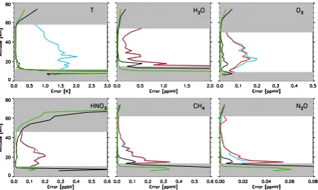
The same analysis has been carried out for other MIPAS main targets (see Sect. 2); results are shown in Fig. 8 with the same format as for O3in Fig. 6. It can be seen in Figs. 6 and 8 that, at altitudes below 30 km, theT-position error is responsible for a meaningful fraction (often exceeding 50 %) of the error due to neglecting the horizontal gradients. 4.4 Propagation to VMR retrievals adopting retrieved
T profiles
We consider now the case in which VMR retrievals are car-ried out usingT profiles that have been determined in a pre-vious step of the analysis (as in MIPAS ground segment). As a first step we have used the simulated retrieval strategy to evaluate the error propagated onT profiles by the horizon-tal homogeneity assumption. The upper-left panel of Fig. 9 shows the RMS of the difference between retrieved and refer-enceT profiles calculated over all the limb-scans of the orbit. As discussed in Sect. 4.1, the geo-location of the retrievedT profiles is identified by the median of theW distribution with respect toT of the analyzed MWs (see the left panel of Fig. 4 for the limb-scan close to the South Pole).
Fig. 8. Same quantities as in Fig. 6 for H2O, HNO3, CH4, and N2O
(see labels).
model to simulate the limb-scan close to the South Pole can be calculated by interpolating the retrievedT profiles on the positions of the red line of Fig. 7. The right panel of this figure also reports, in blue, the position of the adjacentT profiles determined as described in Sect. 4.1 (see Fig. 4).
By analogy with Figs. 6 and 8, the other five panels of Fig. 9 refer to the VMR targets (see labels) and report the RMS of the difference between retrieved and reference pro-files when the retrieved T profiles are used as such (blue lines) and when theT-position errors have been corrected with the interpolation strategy between retrievedT profiles (red lines).
5 Discussion
5.1 Propagation ofT-position error
In Fig. 9 we notice that: (i) the horizontal homogeneity as-sumption leads to significant errors in the retrievedT profiles (of the order of 1–2 K), (ii) the propagation of theseT errors in the retrieved VMR profiles is surprisingly small: the am-plitude of blue lines in Fig. 9 is of the order of 50 % of the corresponding lines in Figs. 6 and 8, (iii) the interpolation strategy implemented to correct for theT-position error does not lead (with the exception of O3)to appreciable improve-ments in the retrieved VMR profiles.
In order to interpret these results we recall that the 1-D retrieval system looks for the profile that better fits the ana-lyzed observations. In the presence of horizontal structures, the reference profiles (that is the profiles used to generate the simulated observations; see Sect. 4.2) do not produce the best fit of the observations. Actually, if we run the simulated T retrieval (upper-left panel of Fig. 9) using the unperturbed reference profiles as initial guess, the value of theχ2 calcu-lated with the initial guess is, on average, 34 times larger than the value calculated at convergence. We then deduce that the 1-D retrieval leads to approximate an “effective” profile that
Fig. 9. Upper-left panel: blue line is the RMS of the difference
be-tween retrieved and referenceT profiles calculated over all the or-bit, black and green lines have the same meaning as in Figs. 6 and 8. Other panels: same quantities as in Fig. 6 for H2O, O3, HNO3, CH4, N2O VMRs obtained using the retrievedT profiles; the red
line is the RMS of the difference profiles when theT-position error has been corrected with the interpolation strategy between retrieved
T profiles.
simulates at best the effect induced by horizontal variability onto the observed spectra. In the case ofT we can say that the behavior of an atmosphere characterized by horizontal T variability is simulated by a horizontally homogeneous at-mosphere described by its “effective”T profile. The retrieved T profile is then more suitable than the reference profile to simulate the radiative properties of the atmosphere within a VMR retrieval. These considerations explain the smaller am-plitude of blue lines in Fig. 9 with respect to the correspond-ing lines in Figs. 6 and 8.
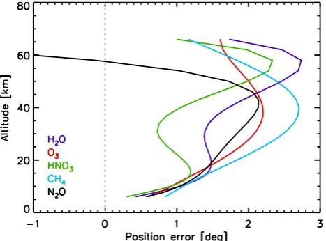
Fig. 10. Average position error of theW distribution with respect toT for the sets of MWs that are analyzed for the retrieval of H2O,
O3, HNO3, CH4, and N2O VMRs.
5.2 Components of the temperature-position error
The maps in Fig. 3 are relative to two different sets of MWs and report the corresponding distribution ofW with respect toT. In both cases it can be seen that the asymmetry with re-spect to the tangent points is quite large. This peculiarity is common to all the sets of analyzed MWs regardless of the tar-get quantity and, therefore, of the MIPAS band where the ob-servations occur. The common asymmetry is also highlighted in Fig. 10 that shows the average position error of theW distribution with respect toT for the sets of MWs that are analyzed by the ground segment for the retrieval of the five MIPAS targets considered in this paper.
We have investigated the origin of the strong asymmetry of theW distributions with respect toT starting from the consideration that, in the radiative transfer process, the values ofT mainly affect the behavior of the source function (the Planck function in our case of local thermodynamic equilib-rium assumption).
In order to understand the relative weight of the source function component in the derivatives of Eq. (1), in Fig. 11 we show theW distribution calculated for the same ob-servations of the left panel of Fig. 3 but forcing to zero the derivatives of the Planck function component. Note that, to better display theW distribution, in Fig. 11 the color scale is expanded by a factor 4 with respect to Fig. 3. The inten-sities and the symmetry observed in Fig. 11 as compared to those in the left panel of Fig. 3, indicate that the derivatives of the Planck function are the main factor responsible for the observed asymmetry of all theW distributions with respect toT. They overwhelm theT derivatives of other elements of the radiative transfer (e.g. the cross-section of the analyzed transitions).
0
12
34
56
Fig. 11.W distribution calculated for the same observations of the left panel of Fig. 3 but forcing to zero the derivatives of the Planck function.
5.3 Position error and averaging kernel
Further evidence of the position errors is provided by the 2-D averaging kernel (AK) relative to a 1-D retrieval (von Clarmann et al., 2009). In this case the position error is highlighted by the offset between the position assigned priori) to the retrieved profile and the position identified (a-posteriori) by the horizontal distribution of the 2-D AK. The size of the position errors estimated using the 2-D AK is con-sistent with the one estimated using the IL analysis. How-ever, the AK is a property of retrieved profiles while the in-formation load is a property of the observations. This makes the IL analysis suitable to identify in advance the layout of the profile that will produce a 2-D AK which is symmetrical with respect to its position. Furthermore, the 2-D AK can-not provide a criterion for the selection of MWs that, when analyzed, minimize the position error of the retrieved profile (see Sect. 3.2) because the AK calculation requires the inver-sion of a matrix that, when defined for a single MW, is often singular.
6 Conclusions
presence of horizontalT gradients, the T-position error is expected to propagate into the retrieved VMR profiles. Sim-ulated retrievals have been used to demonstrate the propaga-tion of theT-position error and to assess its magnitude. In the case of externally-providedT profiles the propagated er-ror is significant especially below 40 km where it can exceed 50 % of the error due to neglecting the horizontal structures. IfT profiles are derived in a first step of the retrieval analysis (this is the case of MIPAS routine retrievals) they suffer by an error (of the order of 1.5 degrees) due to the horizontal homogeneity assumption that affects the accuracy of these profiles if they have to be considered as retrieval products. However, the 1-D retrieval leads to determine “effective”T profiles that simulate the effect induced by horizontal vari-ability onto the observed spectra. For this reason the retrieved T profiles provide satisfactory performance within the VMR retrievals. Furthermore, if T profiles are first retrieved the propagation of theT-position error into the target VMR pro-files is of minor entity. This unexpected result is explained by the IL analysis that shows good matching between the po-sition of the retrievedT profile and the position where this profile is required by the VMR analysis.
We have shown that the information load analysis also pro-vides a tool for the selection of observations (MWs in the case of MIPAS) that, when analyzed, minimize the position error of the retrieved profile.
A strong asymmetry is common to all the horizontal distri-butions ofW with respect toT, independent from the ana-lyzed observations. We have shown that theT dependence of the Planck function is responsible for this asymmetry rather than the T dependence of other elements of the radiative transfer (e.g. the cross-section of the analyzed transitions).
The analysis strategy that we have used in this study can be extended to the 1-D inversion of observations acquired by any limb sounder.
Acknowledgements. E. A. acknowledges the support by ESA
through the CHIMTEA project within the framework of the Changing Earth Science Network Initiative.
Edited by: J. Joiner
References
Beer, R. and Glavich, T. A.: Remote sensing of the troposphere by infrared emission spectroscopy, in: Advanced Optical Instrumen-tation for Remote Sensing of the Earth’s Surface from Space, edited by: Duchossois, G., Herr, F. L., and Zander, R., Proc. SPIE, 1129, 42–51, 1989.
Carlotti, M.: Global-fit approach to the analysis of limb-scanning atmospheric measurements, Appl. Optics, 27, 3250–3254, 1988. Carlotti, M. and Magnani, L.: Two-dimensional sensitivity analysis
of MIPAS observations, Opt. Express, 17, 5340–5357, 2009.
Carlotti, M., Dinelli, B. M., Raspollini, P., and Ridolfi, M.: Geo-fit approach to the analysis of limb-scanning satellite measure-ments, Appl. Optics, 40, 1872–1885, 2001.
Carlotti, M., Brizzi, G., Papandrea, E., Prevedelli, M., Ridolfi, M., Dinelli, B. M., and Magnani, L.: GMTR: Two-dimensional geo-fit multitarget retrieval model for Michelson Interferometer for Passive Atmospheric Sounding/Environmental Satellite observa-tions, Appl. Optics, 45, 716–727, 2006.
Carlotti, M., Castelli, E., and Papandrea, E.: Two-dimensional performance of MIPAS observation modes in the upper-troposphere/lower-stratosphere, Atmos. Meas. Tech., 4, 355– 365, doi:10.5194/amt-4-355-2011, 2011.
Dinelli, B. M., Arnone, E., Brizzi, G., Carlotti, M., Castelli, E., Magnani, L., Papandrea, E., Prevedelli, M., and Ridolfi, M.: The MIPAS2D database of MIPAS/ENVISAT measurements re-trieved with a multi-target 2-dimensional tomographic approach, Atmos. Meas. Tech., 3, 355–374, doi:10.5194/amt-3-355-2010, 2010.
Dudhia, A., Jay, V. L., and Rodgers, C. D.: Microwindow selection for high-spectral-resolution sounders, Appl. Optics, 41, 3665– 3673, 2002.
Fischer, H., Birk, M., Blom, C., Carli, B., Carlotti, M., von Clar-mann, T., Delbouille, L., Dudhia, A., Ehhalt, D., EndeClar-mann, M., Flaud, J. M., Gessner, R., Kleinert, A., Koopman, R., Langen, J., L´opez-Puertas, M., Mosner, P., Nett, H., Oelhaf, H., Perron, G., Remedios, J., Ridolfi, M., Stiller, G., and Zander, R.: MIPAS: an instrument for atmospheric and climate research, Atmos. Chem. Phys., 8, 2151–2188, doi:10.5194/acp-8-2151-2008, 2008. Goldman, A., Murcray, D. G., Murcray, F. J., Williams, W. J., and
Brooks, J. N.: Distribution of water vapor in the stratosphere as determined from balloon measurements of atmospheric emission spectra in the 24–29-µm region, Appl. Optics, 12, 1045–1053, 1973.
ESA: Candidate Earth Explorer Core Missions – Report for Assess-ment: PREMIER – PRocess Exploitation through Measurements of Infrared and millimetre-wave Emitted Radiation, SP-1313/5, ESA Publications Division, ESTEC, Keplerlaan 1, 2200 AG No-ordwijk, The Netherlands, 2008.
Kiefer, M., Arnone, E., Dudhia, A., Carlotti, M., Castelli, E., von Clarmann, T., Dinelli, B. M., Kleinert, A., Linden, A., Milz, M., Papandrea, E., and Stiller, G.: Impact of temperature field inho-mogeneities on the retrieval of atmospheric species from MIPAS IR limb emission spectra, Atmos. Meas. Tech., 3, 1487–1507, doi:10.5194/amt-3-1487-2010, 2010.
Livesey, N. J. and Read, W. G.: Direct Retrieval of Line-of-Sight Atmospheric Structure from Limb Sounding Observations, Geo-phys. Res. Letters, 27, 891–894, 2000.
Puk¸¯ıte, J., K¨uhl, S., Deutschmann, T., Platt, U., and Wagner, T.: Ac-counting for the effect of horizontal gradients in limb measure-ments of scattered sunlight, Atmos. Chem. Phys., 8, 3045–3060, doi:10.5194/acp-8-3045-2008, 2008.
Raspollini, P., Belotti, C., Burgess, A., Carli, B., Carlotti, M., Cec-cherini, S., Dinelli, B. M., Dudhia, A., Flaud, J.-M., Funke, B., H¨opfner, M., L´opez-Puertas, M., Payne, V., Piccolo, C., Reme-dios, J. J., Ridolfi, M., and Spang, R.: MIPAS level 2 operational analysis, Atmos. Chem. Phys., 6, 5605–5630, doi:10.5194/acp-6-5605-2006, 2006.
Hauglustaine, D.: MIPAS reference atmospheres and compar-isons to V4.61/V4.62 MIPAS level 2 geophysical data sets, At-mos. Chem. Phys. Discuss., 7, 9973–10017, doi:10.5194/acpd-7-9973-2007, 2007.
Ridolfi, M., Carli, B., Carlotti, M., von Clarmann, T., Dinelli, B. M., Dudhia, A., Flaud, J.-M., H¨opfner, M., Morris, P. E., Raspollini, P., Stiller, G., and Wells, R. J.: Optimized forward model and re-trieval scheme for MIPAS near-real-time data processing, Appl. Optics, 39, 1323–1340, 2000.
Steck, T., H¨opfner, M., von Clarmann, T., and Grabowski, U.: Tomographic retrieval of atmospheric parameters from infrared limb emission observations, Appl. Optics, 44, 3291–3301, 2005. von Clarmann, T., De Clercq, C., Ridolfi, M., H¨opfner, M., and Lambert, J.-C.: The horizontal resolution of MIPAS, Atmos. Meas. Tech., 2, 47–54, doi:10.5194/amt-2-47-2009, 2009.
Waters, J., Read, W. G., Froidevaux, L., Jarnot, R. F., Cofield, R. E., Flower, D. A., Lau, G. K., Pickett, H. M., Santee, M. L., Wu, D. L., Boyles, M. A., Burke, J. R., Lay, R. R., Loo, M. S., Livesey, N. J., Lungu, T. A., Manney, G. L., Nakamura, L. L., Perun, V. S., Ridenoure, B. P., Shippony, Z., Siegel, P. H., Thurstans, R. P., Harwood, R. S., Pumphrey, H. C., and Filipiak, M. J.: The UARS and EOS Microwave Limb Sounder Experiments, J. Atmos. Sci., 56, 194–218, 1999.