https://doi.org/10.5194/amt-10-4705-2017 © Author(s) 2017. This work is distributed under the Creative Commons Attribution 3.0 License.
Development and application of a backscatter lidar forward
operator for quantitative validation of aerosol dispersion models
and future data assimilation
Armin Geisinger1, Andreas Behrendt1, Volker Wulfmeyer1, Jens Strohbach1, Jochen Förstner2, and Roland Potthast2 1Institute of Physics and Meteorology, University of Hohenheim, Stuttgart, Germany
2Headquarter of the German Weather Service, Offenbach, Germany
Correspondence to:Armin Geisinger ([email protected]) Received: 2 May 2017 – Discussion started: 17 May 2017
Revised: 14 September 2017 – Accepted: 6 October 2017 – Published: 5 December 2017
Abstract.A new backscatter lidar forward operator was de-veloped which is based on the distinct calculation of the aerosols’ backscatter and extinction properties. The forward operator was adapted to the COSMO-ART ash dispersion simulation of the Eyjafjallajökull eruption in 2010. While the particle number concentration was provided as a model output variable, the scattering properties of each individual particle type were determined by dedicated scattering calcu-lations. Sensitivity studies were performed to estimate the uncertainties related to the assumed particle properties. Scat-tering calculations for several types of non-spherical par-ticles required the usage of T-matrix routines. Due to the distinct calculation of the backscatter and extinction prop-erties of the models’ volcanic ash size classes, the sensi-tivity studies could be made for each size class individu-ally, which is not the case for forward models based on a fixed lidar ratio. Finally, the forward-modeled lidar profiles have been compared to automated ceilometer lidar (ACL) measurements both qualitatively and quantitatively while the attenuated backscatter coefficient was chosen as a suitable physical quantity. As the ACL measurements were not cal-ibrated automatically, their calibration had to be performed using satellite lidar and ground-based Raman lidar measure-ments. A slight overestimation of the model-predicted vol-canic ash number density was observed. Major requirements for future data assimilation of data from ACL have been iden-tified, namely, the availability of calibrated lidar measure-ment data, a scattering database for atmospheric aerosols, a better representation and coverage of aerosols by the ash dis-persion model, and more investigation in backscatter lidar forward operators which calculate the backscatter coefficient
directly for each individual aerosol type. The introduced for-ward operator offers the flexibility to be adapted to a multi-tude of model systems and measurement setups.
1 Introduction
In spring 2010, the Icelandic volcano Eyjafjallajökull erupted several times. The emitted ash was found to be harmful for aircraft, and due to uncertain information about spatial dis-tribution and concentration of volcanic ash, the European air space was closed for several days (Sandrini et al., 2014). The high economic costs and impact on public transport led to ef-forts of DWD (Deutscher Wetterdienst) to improve monitor-ing and predictmonitor-ing ash plumes in the atmosphere. Therefore, DWD decided to start a dedicated project on backscatter li-dar forward operators for validating aerosol dispersion mod-els using available remote-sensing measurement data and for future assimilation of lidar backscatter and extinction data.
Emeis et al., 2011), MesoNH (Non-Hydrostatic Mesoscale Atmospheric Model of the French Research Community; Mallet et al., 2009), and WRF-CHEM (Weather Research and Forecast Model; Chen et al., 2014). Using these model systems, scientists have analyzed the aerosol influence on, for example, precipitation (Rieger et al., 2014), temperature (Bangert et al., 2012), radiative fluxes (Vogel et al., 2009), and convection initiation (Chaboureau et al., 2011). These models are potentially capable of simulating such ash disper-sion scenarios and could thus benefit from the methodology presented here.
Lidar (light detection and ranging) is capable of providing information on atmospheric particles with high temporal and spatial resolution. The most basic lidar type is the backscat-ter lidar which measures the backscatbackscat-tered signal intensity of a volume at a certain range. Comparing the data of such a backscatter lidar that is operated in the UV with simulations of an atmospheric chemistry model allows for the character-ization of transport and optical properties of aerosol parti-cles near sources (Behrendt et al., 2011; Valdebenito B et al., 2011). Using ground-based DIAL (differential absorption li-dar; Weitkamp, 2008; Späth et al., 2016) water-vapor can be measured, which can even be combined with backscat-ter measurements to derive more details of aerosol parti-cle properties (Wulfmeyer and Feingold, 2000). Lidar tech-niques based on the vibrational and rotational Raman effect, like RRL (rotational Raman lidar) allow for the measurement of trace gas profiles (Whiteman et al., 1992; Turner et al., 2002; Wulfmeyer et al., 2010; Haarig et al., 2016) as well as profiles of atmospheric temperature, particle backscatter cross section, particle extinction cross section, and particle depolarization properties (Behrendt et al., 2002; Hammann et al., 2015; Radlach et al., 2008). High-spectral-resolution lidar (HSRL) systems furthermore allow for cloud and parti-cle characterization (Shipley et al., 1983). Multi-wavelength lidar systems offer the potential to retrieve the optical, mi-crophysical, and chemical properties of aerosols (Mamouri et al., 2012), but these systems are rare and the inversion al-gorithms are very complex. Profiles of the radial wind speed can be obtained by using Doppler–lidar systems (see, e.g., Banta et al., 2012).
While the number of sophisticated lidar instruments that provide thermodynamic data (Wulfmeyer et al., 2015) is still low, there are already automated aerosol lidar networks in operation in Europe and Asia (Pappalardo et al., 2014; Sugi-moto et al., 2008). The data of such networks offer 3-D parti-cle information with high temporal and vertical and moderate horizontal resolution. Automated ceilometer lidar systems (ACLs) have been used to detect cloud and boundary layer heights (Emeis et al., 2009) but the received signal also de-livers information about aerosols. It is therefore worthwhile to use the ACL network measurements for the validation of particle transport model simulations. Unfortunately, it is not possible to obtain the particle number concentration from an elastic backscatter signal alone without ancillary information
and assumptions which are partly critical. The alternative is to use the detailed atmospheric description of the model to simulate lidar profiles for a model-given atmospheric state. Such a lidar simulator is called a lidar forward operator. Us-ing an ideal lidar forward operator, the signal of a given lidar system can be calculated from the model prediction at any time interval, grid location, and measurement direction.
There are already several backscatter lidar forward oper-ators available or in development which are based on the calculation of the extinction coefficient. The backscatter co-efficient is then calculated assuming a given lidar ratioSlidar (Benedetti, 2009; Morcrette et al., 2009; Siˇc, 2014; Charlton-Perez et al., 2013; Lange and Elbern, 2014). On the one hand, this method benefits from the fact that the extinction coeffi-cient is less sensitive to the particle dimension and shape than the backscatter coefficient. On the other hand, the precision of this method is limited to the correctness of assumed lidar ratio values. The method becomes unusable once there is a mixture of scatterers.
We designed a forward operator which is based on the dis-tinct calculation of exdis-tinction and the backscatter coefficients in the model system. This forward operator can be adapted to particle-representing atmospheric model and backscatter li-dar systems even using multiple wavelengths. It has the capa-bility to calculate both the attenuated backscatter coefficient and the lidar ratio from model output data with a minimum set of external information. The name of the forward model is “backscatter lidar forward operator” (BaLiFOp).
In the following we explain the lidar principles and the the-oretical background for the backscatter lidar forward opera-tor (Sect. 2). This is followed by an introduction to the case study in Sect. 3. Sensitivity studies of the particles’ scattering properties are presented in Sect. 4. Results of the forward op-erator and a comparison to ACL measurement data are shown in Sect. 5. Finally, we summarize the results of our study and discuss both the benefits and the requirements of current and future lidar data assimilation systems (Sect. 6).
2 Methods
2.1 The lidar equation
The lidar principle is based on the emission of laser pulses into the atmosphere and the measurement and analysis of the backscatter signals. The received photon number per pulse Nrec,λ(z) from rangezis described by the following
equa-tion for elastic backscatter lidars which detect the backscatter signal at the emitted wavelength:
Nrec,λ(z)= (1)
Ntr,λ τ c
2 ηλO(z) Atel
z2 βλ(z)exp
−2
z
Z
0
αλ(z0)dz0
Instrument-dependent variables of the lidar equation are the wavelengthλ, the laser emitted photon number per pulse Ntr,λ, the temporal length of a laser pulseτ, the efficiency of
the receiving system and detectorsηλ, the overlap function O(z), and the net area of the receiving telescope Atel. The received signal intensity can be given either as power or in photon counts. Here, we use photon counts per laser pulse unless otherwise noted.
The range resolution is usually matched to the temporal resolution of the data acquisition system by τ c2 =1zwith cas speed of light. Typical1zvalues for ACL systems are a few meters. The overlap function O(z)is 0 (no overlap) near the ground and becomes 1 (full overlap) above a cer-tain height, which is typically 200 to 1500 m above ground for ACL systems (Wiegner et al., 2014; Flentje et al., 2010a). The missing overlap limits the capability to measure and cal-ibrate in the near range but has no effect where full overlap has been accomplished. Heights where 0< O(z) <1 can be overlap-corrected if the device-specific overlap function is known.
Processes in the atmosphere are described by the backscat-ter coefficientβλ(z)and the extinction coefficientαλ(z). The
backscatter coefficientβλ(z)describes the scattering strength
into the direction of the receiving telescope and depends on wavelength, type, shape, and size of scatterers, and their re-spective number concentrations; βλ(z) is given in units of
m−1sr−1. The extinction coefficient αλ(z)is a description
for laser radiation absorption and scattering capabilities of objects in a volume; it is given in units of m−1.
Elastic backscatter lidar systems do not allow for a sepa-rate measurement ofβλ(z)andαλ(z)as two unknowns
can-not be determined with one measured variable. For calibrated backscatter lidar systems, it is thus convenient to calculate the attenuated backscatter coefficient γλ(z) from the
mea-sured profiles:
γλ(z)=βλ(z)exp
−2
z
Z
0
αλ(z0)dz0
. (2)
It is given in units of m−1sr−1. The attenuated backscatter coefficient is independent of all instrument-specific parame-ters except the wavelength. Therefore, it is the best suitable physical quantity for comparison between backscatter lidar measurement and aerosol model using a forward operator as long as no ACL measurements of extinction and backscatter cross section profiles are available for this purpose.
2.2 The backscatter lidar forward operator
According to Eq. (2), the basic functionality of the forward operator is the calculation of extinction coefficientαλ(z)and
backscatter coefficient βλ(z) based on a given atmospheric
state and, finally, to determine the attenuated backscatter co-efficientγλ(z).
2.2.1 Scattering of laser radiation by arbitrary objects The total extinction coefficientαλ(z)and the total
backscat-ter coefficientβλ(z)of an illuminated volume withqs
differ-ent types of scatterers are calculated from
αλ(z)= qs
X
i=1
αi,λ(z)= qs X i=1 ∞ Z 0
ni(R, z)σext,i,λ(R)dR, (3)
βλ(z)= qs
X
i=1
βi,λ(z) (4)
= qs X i=1 ∞ Z 0
ni(R, z)
d
σsca,i,λ(R)
d
π
dR,
whereni(R, z) is the number-size distribution of scatterer
typeiwith radiusRat rangezgiven in units of m−3,σext,i,λ
is the corresponding extinction cross section given in units of m2, anddσsca,i,λ
d
π is the differential backscatter cross
sec-tion given in units of m2sr−1.
For isotropic scattering, the differential backscatter cross section is derived from the scattering cross sectionσsca,i,λ(R)
via
dσ
sca,i,λ(R)
d
π
=σsca,i,λ(R)
4πsr . (5)
For non-isotropic scattering, a phase functionφi,λ(θ, R)is
used to describe the relative scattering intensity into angleθ, which isπfor monostatic systems:
dσ
sca,i,λ(R)
d
π
=σsca,i,λ(R)
4πsr φi,λ(π, R). (6)
Molecule scattering and particle scattering are differenti-ated here, as the respective calculations depend on suitable physical theories and algorithms.
2.2.2 Scattering by molecules
For a model which is capable of distinguishing atmospheric gases such as nitrogen, oxygen, argon, and water vapor, the molecule scattering calculation could be performed for each individual gas type and molecule size using the Rayleigh the-ory (Young, 1981). For ACL systems, provided that a wave-length is used which is well outside of molecular absorption lines, the individual gas contribution to the signal does not need to be distinguished.
Consequently, the molecule extinction coefficient αmol,λ(z)and the molecule backscatter coefficientβmol,λ(z)
can be calculated with
αmol,λ(z)=Nmol,λ(z)σsca,mol,λ, (7) βmol,λ(z)=Nmol,λ(z)
dσ
sca,mol,λ
d
π
where the molecule number densityNmol(z)is related to the ideal gas law
Nmol(z)= p(z)
k T (z), (9)
with p as atmospheric pressure given in pascal (Pa), T as temperature given in kelvin (K), and k as Boltzmann con-stant, which has a value of 1.38×10⁻²³J K−1.
To calculate the scattering cross sectionσsca,mol,λand the
scattering phase functionφa,λ(θ )of air, we used the
formu-las and look-up tables given by Buchholtz (1995). As these empirical equations are only provided for wavelengths up to 1000 nm, we simply extrapolated the values to the ACL wavelength in the case study (1064 nm).
2.2.3 Scattering by particles
The scattering characteristics of larger particles are described by Mie’s solution of the Maxwell equations (Mie, 1908; Wiscombe, 1980). The T-matrix method (Mishchenko et al., 2002) or the discrete dipole approximation (DDA; Draine and Flatau, 1994) allow for calculating the scattering prop-erties of non-spherical objects with sizes not much smaller or larger than the wavelength. The T-matrix method is a tool for computing scattering by single and compounded particles (Mishchenko et al., 2002). It is faster than DDA but limited to rotationally symmetric objects such as ellipsoids, cylinders, or Chebyshev polynomials. DDA, however, has the flexibil-ity to represent arbitrarily shaped objects at the cost of high computational efforts.
As a rough estimate, the computational time increases by about 1 order of magnitude when using T-matrix instead of Mie scattering calculation routines and by another 2 orders of magnitude when using DDA instead of T-matrix. Another increase in computational time results from larger scatterers; i.e., an increase in the particle size results in an exponential increase in computing time. In this study, Mie scattering al-gorithms are therefore used to perform fast calculations. The effect of scattering by non-spherical particles is analyzed in a second step by T-matrix scattering calculations for several non-spherical particle shapes in the framework of sensitivity studies. This approach is required because the COSMO-ART volcanic plume simulation does not output any information about the particle shape distribution.
Mie scattering-related computations were performed using the IDL (Interactive Data Language) procedure “mie_single”, provided by the Department of Atmospheric, Oceanic and Planetary Physics (AOPP), University of Ox-ford. Input parameters of the procedure are the real partm and imaginary partm0of the refractive index as well as the so-called size parameterXλ(R):
Xλ(R)=
2π R
λ , (10)
whereRis the radius of a single particle. The relevant output parameters are the extinction efficiencyQext,p,λ(R)and the
backscatter efficiencyQbsc,p,λ(R)of particle typep. These
optical efficiencies are defined as ratio between the optical cross section and the physical cross section:
Qext,p,λ(R)=
σext,p,λ(R)
π R2 , (11)
Qbsc,p,λ(R)=
dσ
sca,p,λ(R) d
π
π R2 . (12)
As a warning, we would like to point out that the pro-cedure changed its definition of the backscatter efficiency: the 2012 release of mie_single returns the so-called radar backscatter efficiency, which is 4πtimes the backscatter effi-ciency we require within the forward operator. Furthermore, the procedure expects the imaginary part of the refractive in-dex given as negative number. If positive imaginary part val-ues are used, the procedure runs without showing an error but returns wrong results.
2.2.4 Discrete particle number size distributions A major problem of discrete size distributions is the high sensitivity of the optical cross sections to the particle size: a slightly different particle radius may lead to quite a large change of the scattering properties. We present in the follow-ing an approach to overcome this problem. Due to the fact that naturally occurring particle size distributions are not dis-crete, averaging the optical cross sections over certain size-intervals seems straightforward. We will show that this ap-proach indeed reduces the problematic and unrealistic sensi-tivity significantly. If the model represents only one type of particle, i.e., with a constant refractive index but with discrete radiiRd, we can define the effective extinction cross section
and the effective backscatter cross sections with
σext,Rd,m,m0,λ= (13)
1 Rdb−Rda
Rdb
Z
Rda
Qext(Xλ(Rd), m, m0)π R2d dRd,
σbsc,Rd,m,m0,λ= (14)
1 Rdb−Rda
Rdb
Z
Rda
Qbsc(Xλ(Rd), m, m0)π Rd2dRd,
whereRda andRdb are size margins for each particle size classd. These integrals are then exchanged with sums in the numerical computation routines.
The calculation of the effective values is performed for ev-ery discrete size classd and – if represented by the model – also for every particle typek. Consequently, the total par-ticle extinction coefficient αpar,λ(z) and the total particle
αpar,λ(z)=
X
k
X
d
Nd,k(z)σext,Rd,mk,m0k,λ, (15) βpar,λ(z)=
X
k
X
d
Nd,k(z)σbsc,Rd,mk,m0k,λ. (16)
Here, Nd,k is the particle number per volume given by the
model, σext,Rd,mk,m0
k,λ and σbsc,Rd,mk,m0k,λ are the effective optical cross sections of particle size classdand particle type classkwith the respective real partmkand imaginary partm0k
of the refractive index.
The forward-modeled total extinction coefficient and total backscatter coefficient are the sum of the molecule and the particle extinction and backscatter coefficients:
αλ(z)=αmol,λ(z)+αpar,λ(z), (17) βλ(z)=βmol,λ(z)+βpar,λ(z), (18)
equivalent to Eqs. (3) and (4). 2.2.5 Two-way transmission
The two-way transmissionTλis calculated from
Tλ(z)=exp
−2
z
Z
0
αλ(z0)dz0
. (19)
Within the forward operator, the two-way transmission is discretized by using the models’ vertical layers as height in-crement and vertical resolution.
2.2.6 Lidar ratio
Even though the lidar ratio is not measured directly by cur-rent ACL systems, the capability of simulating the lidar ratio for given scatterer types and scatterer mixtures offers great potential for sensitivity studies but also for comparison to research lidar systems such as Raman lidar. The forward-modeled total lidar ratioSlidar(z)can be calculated from Slidar,λ(z)=
αpar,λ(z) βpar,λ(z)
, (20)
whereαpar,λ(z)andβpar,λ(z)are the total particle extinction
and backscatter coefficients given by Eqs. (15) and (16), re-spectively. This depends not only on the assumed particle type and shape, but also on the particle size class configu-ration of the model, i.e., size class number, size class range, and particle size coverage. The forward-modeled lidar ratio thus becomes more representative with a wider particle size spectrum as well as with greater particle size, type, and shape classes output by the dispersion model.
To analyze the lidar ratio sensitivity independent of a mod-els’ particle size class and type class configuration, we in-troduced the pure lidar ratio Slidar,pure. In a molecule-free
volume with monodisperse particles, the particle number per volumeNR,p, withRas particle radius, cancels, giving Slidar,pure,R,p,λ=
σext,R,p,λ σbsc,R,p,λ
. (21)
The pure lidar ratio Slidar,pure,R,p,λ allows for performing
sensitivity studies to analyze influences of the particle shape on the expected lidar ratio values (Sect. 4).
3 Case study 3.1 Description
The 2010 Eyjafjallajökull eruption was extensively analyzed by scientists from many fields of research, resulting in a substantial knowledge base (see ACP special issue “Atmo-spheric implications of the volcanic eruptions of Eyjafjalla-jökull, Iceland 2010”). Ash layers were observed from a large set of measurement instruments, allowing for tracking of the volcanic ash plume over Europe (Gasteiger et al., 2011a; Za-kšek et al., 2013; Mona et al., 2012; Dacre et al., 2013; Wa-quet et al., 2014). Using images from the geostationary in-strument SEVIRI (Spinning Enhanced Visible and Infrared Imager) the spatial extent of the ash plumes and their move-ments could be tracked and compared to the measurement of ground-based instruments (Strohbach, 2015; see Fig. 1). From the synergy of the two measurement systems, layers with strong backscattering measured by ACL systems could be related to clouds or volcanic ash layers.
In terms of dispersion modeling, such a volcanic eruption case has a well-known aerosol source location. This feature renders the Eyjafjallajökull eruption an important case study for aerosol dispersion simulation models and respective val-idation methods (Matthias et al., 2012).
3.2 The DWD ACL network
ACL networks are a valuable data source for analyzing the vertical and horizontal structure of aerosol particles, model verification, and data assimilation. A qualitative analysis of the Eyjafjallajökull ash plume over Germany using obser-vations from 36 ACL systems CHM15k manufactured by Jenoptik (currently known as Lufft) was performed by Flen-tje et al. (2010a).
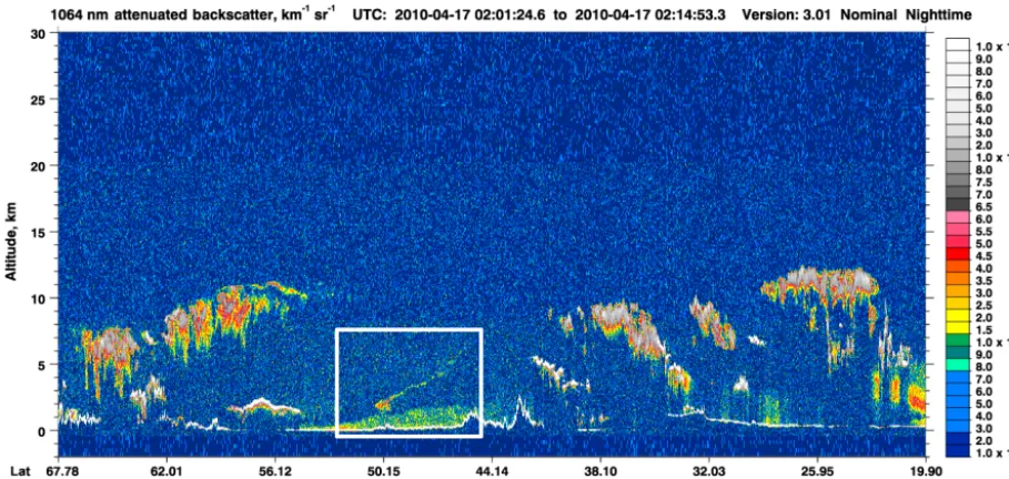
Figure 1.Distribution and transport of volcanic ash over northwest Europe sketched using georeferenced satellite images (Meteosat-9, Dust). After georeferencing, the ash layers were retraced as colored polygons, where the color of the polygons (yellow to red) represent consecutive time steps (Strohbach, 2015). The blue dashed line indicates the flight track of CALIPSO during 17 April 2010 (measurement shown in Fig. 2).
The received photon number per shot is calculated from Nrec(z, t )=beta_raw(z, t )·SD(t )+base(t ), (22) where beta_raw is the signal-to-noise measurement product, SD is noise, and base is a daylight correction provided by the ACL software of this model.
The equation for calculating the attenuated backscatter co-efficient from ACL-measured photon counts reads
γλ(z)=
Nrec,λ(z, t )z2 Ntr,ληλAtelO(z)1z
. (23)
The pulse energy of the diode-pumped laser is 8 µJ (Flen-tje et al., 2010b) resulting in an emitted photon number per pulse of about 4.28×10¹³. The diameter of the receiving telescope is 100 mm (Flentje et al., 2010b) which results inAtel=78.54 cm2. The vertical resolution1zis 15 m for the complete profile. The overlap functionO(z)was set to 1 which implies that ranges below about 1500 m cannot be used reliably for comparisons with the forward operator.
Unfortunately, the instruments provided no calibrated measurement data at that time, so a linear calibration fac-torη∗ is used as replacement for the system efficiencyηλ.
From a comparison with calibrated attenuated backscatter measurements of CALIOP at λ=1064 nm (Fig. 2), a cal-ibration factor of η∗=0.003 could be determined; there-fore, the CALIOP value of the 1064 nm calibrated atten-uated backscatter coefficient was used at 50.15◦, 4.81◦ at
a height of 2 km. As a validation step, the resulting atten-uated backscatter coefficient values were compared to Ra-man lidar measurements of the volcanic ash plume at Mu-nich and Leipzig (Ansmann et al., 2010). The maximum Ra-man lidar measured backscatter coefficient atλ=1064 nm was 8×10⁻⁶m−1sr−1 for both Munich and Leipzig and the maximum calculated attenuated backscatter coefficient of the ACL measurement at Deuselbach after calibration is of the same order of magnitude. As most present ACL net-works have been extended by automatic calibration capabil-ities, such pragmatic calibration approaches will not be re-quired in future forward operator studies. It should be noted that it is not only the absolute calibration which is important. Even if the calibration is not perfect, a comparison of lidar and model data permits a thorough comparison of vertical structures such as the thickness and heights of aerosol layers. As a last step, the high-resolution ACL data was gridded to the model’s vertical resolution and to 15 min time steps. This also improved the signal-to-noise ratio of the ACL data. 3.3 Ash transport simulation of COSMO-ART
Figure 2.Attenuated backscatter coefficient measurement from CALIOP used to calibrate the ACL measurement during the Eyjafjallajökull eruption phase. The volcanic ash plume is visible around 50.15◦, 4.81◦. As the instrument measures from space, the values of the attenuated backscatter coefficient inside the ash plume is not affected by attenuation due to aerosols in the planetary boundary layer. Image obtained from http://www-calipso.larc.nasa.gov/.
Figure 3. Sketch of the particle size distribution represented by COSMO-ART for the Eyjafjallajökull dispersion simulation (red dots). The red lines with bars indicate the averaging margins that were defined for the calculation of effective optical cross sections.
size of 7 km and 40 height layers. The height layer thickness was variable, ranging from several meters near the ground to a layer thickness of about 3 km at 22 km height above ground level. A more general description of the model run is given by Vogel et al. (2014).
For this study, the 78 h forecast was used, beginning on 15 April 2010, 00:00 UTC, which includes volcanic ash emission data starting from 14 April 2010, 06:00 UTC. Vol-canic ash was represented by six discrete size classes with
aerodynamic diameters of 1, 3, 5, 10, 15, and 30 µm. For each class, a number concentration was predicted by the model. Particles within a class were treated as being identical, i.e., having the same size, shape, and complex index of refraction (monodisperse distribution), so the calculation of effective optical cross sections follows Sect. 2.2.4. The lower and up-per size marginsRda andRdb were defined as arithmetic av-erages of two subsequent size classes. The lower margin of the smallest size class was half its nominal diameter; the up-per margin of the largest size class was 1.5 times its nominal diameter. The resulting class ranges are shown in Fig. 3. A list of model variables used for the forward operator is given by Table 1.
3.4 Volcanic ash properties
A detailed analysis of the emitted ash was performed by Schumann et al. (2011) who compared measurements from the DLR Falcon 20 aircraft with data of research lidar sys-tems in Germany. Eyjafjallajökull ash samples were taken in situ, analyzed using a scanning electron microscope, and as-signed to matter groups. From the matter components, the complex index of refraction was calculated.
Table 1. Output variables of COSMO-ART used by the forward operator for the selected case study.
Variable Symbol Description Unit
ASH1 N1 Ash number density of m−3 class 1 (1 µm)
ASH2 N2 Ash number density of m−3 class 2 (3 µm)
ASH3 N3 Ash number density of m−3 class 3 (5 µm)
ASH4 N4 Ash number density of m−3 class 4 (10 µm)
ASH5 N5 Ash number density of m−3 class 5 (15 µm)
ASH6 N6 Ash number density of m−3 class 6 (30 µm)
Pmain p Atmospheric pressure hPa
T T Atmospheric temperature ◦C
Electron microscope images from the same study revealed that the volcanic ash particles were sharp edged with a com-plex and asymmetric shape. The average asymmetry factor was 1.8 for small particles (<0.5 µm) and 2.0 of larger parti-cles (Schumann et al., 2011). Electron microscope measure-ments of Rocha-Lima et al. (2014) showed that the asymme-try factor of the volcanic ash fine fraction was between 1.2 and 1.8.
The particle growth due to hygroscopic water coating was quantified to be about 2 to 5 % at a relative humidity of 90 % (Lathem et al., 2011). A growth of 5 % does not change the scattering properties significantly in relation to the size av-eraging which is performed for monodisperse size classes in the forward operator. But even perfectly known volcanic ash particles will change their constitution while traveling through the atmosphere. It is therefore essential to analyze the maximum uncertainty for applying the forward opera-tor on volcanic ash particles with variable properties, namely particle size, refractive index, and shape.
4 Sensitivity studies
The representation of the particles by the model is clearly simplified, so the effect of these simplifications on the scat-tering of laser light must be determined when applying the forward operator. For a lidar forward model, sensitivities of the backscatter cross section are critical because the received signal intensity is linearly coupled to the backscatter cross section and, consequently, to the attenuated backscatter co-efficient.
Prior studies already showed the complexity of non-spherical scattering calculations but there is no universal solution to the problem available. Gasteiger et al. (2011b) used DDA to calculate the scattering properties of
complex-shaped particles but the analysis was limited to size parame-ters up to 20.8 due to the increasing computational time per iteration for increasing particle sizes. The equivalent radius at a wavelength of 1064 nm would be 3.5 µm. The compu-tation of a high-resolution multi-dimensional look-up table for up to 10 times larger particles would require an unfea-sible amount of time. The study of Kemppinen et al. (2015) focused on individual ellipsoids but assuming an ellipsoidal distribution to represent fractional and sharp-edged parti-cles may lead to less realistic scattering calculation results than assuming spherical scatterers. Consequently, there is no scattering description for Eyjafjallajökull ash predictions of COSMO-ART available. Thus, we decided to treat the vol-canic ash as spherical objects with given optical properties (see Sect. 3.4), but we nevertheless analyze and discuss the effect of variable volcanic ash properties in the following.
It must be noted that these studies are required for most aerosol types as most naturally occurring aerosols are not perfectly spherical and even slightly non-spherical ellipsoids may have very different scattering characteristics compared to ideal spheres.
4.1 Prerequisites
Look-up tables (LUTs) of Mie efficiencies and optical cross sections have been created to reduce the effort spent on time-consuming scattering calculations. The look-up tables have three dimensions: size parameterXλ(Rp), real part of the re-fractive indexm, and imaginary part of the refractive index m0.
The reasonable range of size parameters depends on the wavelength of the lidar transmitters and the radius of oc-curring particlesRp. For the ACL systems operating atλ= 1064 nm, we get a size parameter range of 1.2 to 142.9 with values of the particle radius of 0.2 to 24.2 µm; see Eq. (10).
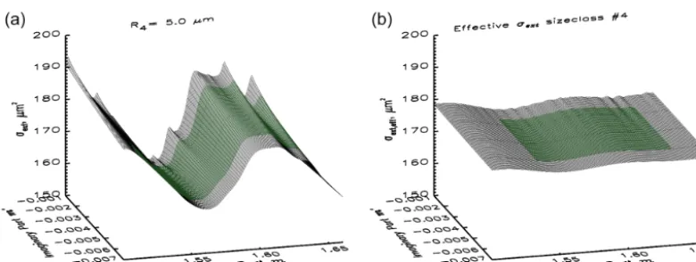
Figure 4.Sensitivity of σextto the real and imaginary part of the refractive index for a single particle radiusRpof 5 µm(a)and after calculating the effective extinction cross sectionσextfor size class 4(b). The green shaded area is the considered range of real partmand imaginary partm0for the uncertainty estimation as explained in Sect. 4.1.
Figure 5.The same as Fig. 4 but for the backscatter cross sectionσbsc(a)and the effective backscatter cross sectionσbsc(b). The backscatter cross section is very sensitive to the refractive index. While the major fraction of backscatter cross section variations can be removed by calculating the effective backscatter cross section, the sensitivity at the extreme end of the defined refractive index remains.
4.2 Sensitivity to the complex index of refraction Extinction cross section σext, backscatter cross sectionσbsc, effective extinction cross sectionσext, and effective backscat-ter cross sectionσbscplotted over real and imaginary parts of the complex index of refraction are shown in Figs. 4 and 5 for a particle radius of 5 µm and class 4 as an example. While the extinction cross sectionσextis more sensitive to the real part than to the imaginary part of the refractive index, the backscatter cross section σbsc is strongly sensitive to both. These sensitivities are strongly reduced for the effective ex-tinction cross sectionσextand the effective backscatter cross sectionσbsc.
A measure for the refractive index sensitivity of the effec-tive optical cross sections is given by Fig. 6, which shows the relative errors
σext,err,p(m, m0)= (24)
σext,p(m, m0)−σext,p(m∗, m0∗) σext,p(m∗, m0∗)
·100 %,
and
σbsc,err,p(m, m0)= (25)
σbsc,p(m, m0)−σbsc,p(m∗, m0∗) σbsc,p(m∗, m0∗)
·100 %.
Figure 6.Relative errors of the effective extinction cross section(a, b)and of the effective backscatter cross section(c, d)if the assumed reference refractive index (1.59−0.004i) varies from the true refractive index. Uncertain real parts of the refractive index(a, c)may lead to errors of 7 % for the effective extinction cross section as well as of 225 % for the effective backscatter cross section. Uncertain imaginary parts of the refractive index(b, d)may lead to a maximum error of 0.5 % for the effective extinction cross section and of 230 % for the effective backscatter cross section. The maximum error was observed at the outer range of considered refractive indices. Therefore, reducing the considered range of refractive indices reduces the maximum error of the effective extinction and backscatter cross section.
4.3 T-matrix particle shape sensitivity study
The T-matrix calculations performed in this study are based on the FORTRAN code for randomly oriented particles, writ-ten and provided by Mishchenko and Travis (1998). A de-tailed description of the method can be found in Mishchenko et al. (2002).
The double-precision version of the T-matrix procedure was modified to perform scattering calculations of multi-ple particle sizes automatically. In addition, the procedure was extended by calculating and returning the backscatter cross section σbsc according to Mishchenko et al. (2002), Eq. (9.10). These modifications were tested by comparing
the scattering calculation results of the modified code and mie_single for spherical particles and the results were iden-tical.
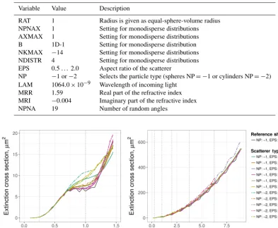
Table 2.Settings of the T-matrix procedure for the particle shape sensitivity study. The parameters were kept constant during the study except the particle shape parameters (EPS and NP).
Variable Value Description
RAT 1 Radius is given as equal-sphere-volume radius NPNAX 1 Setting for monodisperse distributions AXMAX 1 Setting for monodisperse distributions B 1D-1 Setting for monodisperse distribution NKMAX −14 Setting for monodisperse distributions NDISTR 4 Setting for monodisperse distributions EPS 0.5 . . . 2.0 Aspect ratio of the scatterer
NP −1 or−2 Selects the particle type (spheres NP= −1 or cylinders NP= −2) LAM 1064.0×10−9 Wavelength of incoming light
MRR 1.59 Real part of the refractive index MRI −0.004 Imaginary part of the refractive index
NPNA 19 Number of random angles
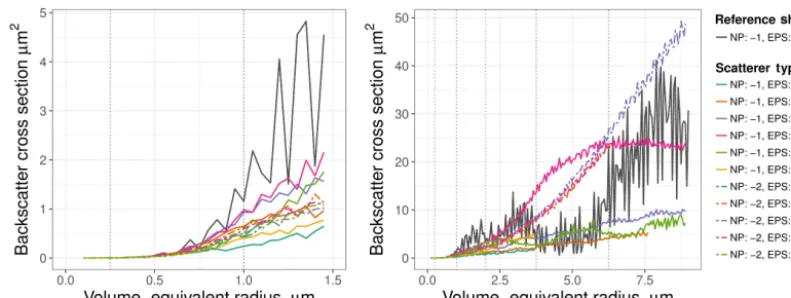
Figure 7.Extinction cross section spectrum for the reference particle (sphere, dark grey line), six types of ellipsoids (EPS=1, solid lines), and five types of cylinders (EPS= −2, dashed lines) against the particles’ equal-volume radiusRpatλ=1064 nm. Vertical dotted lines indicate the size margins of each class. The particle shape effect is negligible for particles with a radius much smaller than the wavelength. Particles which have a radius equal to the wavelength show differences of the extinction cross section depending on their shape. With larger particle sizes, the particle shape effect is negligible for the considered shapes and aspect ratios.
In Figs. 7, 8, and 9, the optical cross sections and the pure lidar ratio of spheres and several aspherical particles are plot-ted against the equal-volume radius. The aspherical scatter-ers are six ellipsoids with a diameter-to-length ratio of 0.50, 0.67, 0.75, 1.25, 1.50, and 2.00 as well as five types of cylin-dric particles with a diameter-to-length ratio of 0.50, 0.80, 1.00, 1.25, and 2.00. Unfortunately, the scattering properties of a highly asymmetric ellipsoid (EPS: 0.50) is only available up to an equal-volume radius of 3.75 µm. For future research activities in this topic, the quadruple precision version of the T-matrix code could be used to extend the upper size range of highly asymmetric particles.
No significant differences between the extinction cross section of spheres and these ellipsoids were observable. The trend is, however, that cylindrically shaped particles have a higher extinction cross section compared to ellipsoids. Spheres have the lowest extinction cross section values over
the whole spectrum. Up to a volume-equivalent radius of 0.7 µm, the shape effect is not noticeable.
Figure 8.The same as Fig. 7 but for the backscatter cross section. A high particle shape sensitivity of the backscatter cross section can be observed which becomes pronounced for particles with radii greater than 0.5λ. While the backscatter cross section of ellipsoids increases only weakly with particle size, the backscatter cross section of cylinders increases near exponentially with size. The backscatter cross section spectrum of spheres has larger-scale fluctuations which are due to interference effects. For particle size classes 4 and 5, the backscatter cross section of spheres is between the values of ellipsoids and cylinders which indicates that a spherical shape is a valid representative for large volcanic ash size classes
Figure 9.The same as Fig. 7 but for the pure lidar ratio. Similar to the observations for the backscatter cross section (see Fig. 8), the particle shape sensitivity of the pure lidar ratio is negligible for particles smaller than 0.5λ. For larger particles, the spherical shape tends to have the lowest pure lidar ratio value of all particle shapes (namely for a particle radius between 0.5 and 3.5 µm). Peaks of the pure lidar ratio are observed for spheres with a radius between 4 and 6 µm which are due to interference effects. Large ellipsoids tend to have the highest pure lidar ratio values in comparison with other particle shapes; large cylinders have an almost constant value of the pure lidar ratio of about 15 sr.
equal-volume radius is greater than 3.75 µm (for the given wavelength ofλ=1064 nm).
The particle shape effect on the pure lidar ratio is weakly pronounced for small particle sizes (less than 0.75 µm). For larger particles, the pure lidar ratio of spheres is generally lower than that of the other considered shapes which is in agreement with the higher backscatter cross section observed before. For the fourth size class (equal-volume radii around 5 µm), the previously observed interference effects of the spheres’ backscatter cross section lead to extreme values of the pure lidar ratio (exceeding a value of 200 sr). For the size classes 2, 3, and 5, however, the pure lidar ratio of spheres is lower than that of all other considered particle shapes except for cylinders. This indicates that the assumption of spherical
scatterers results in an underestimation of the total lidar ratio if the considered particles are not spherical, and size classes 2, 3, and 5 contribute predominately to the total volcanic ash number density.
NP: −2 NP: −1
1 2 3 4 1 2 3 4 −40 %
−20 % 0 % 20 %
Particle size class number
Relativ
e diff
erence
σext,err
Aspect ratio
0.50
0.67
0.75
0.80
1.00
1.25
1.50
2.00
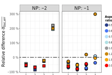
Figure 10.Relative errors of the effective extinction cross section if spherical particles are assumed but real particles have an elliptical (NP:−1) or cylindrical shape (NP:−2). Negative values indicate that spherical particles have a larger effective extinction cross sec-tion than equal-sized non-spherical particles and vice versa. The maximum relative differences are+11 and−35 %.
NP: −2 NP: −1
1 2 3 4 1 2 3 4 −100%
0% 100% 200% 300%
Particle size class number
Relativ
e diff
erence
σbsc
,err
Aspect
ratio 0.50
0.67
0.75
0.80
1.00
1.25
1.50
2.00
Figure 11.The same as Fig. 10 but for the effective backscatter cross section. The maximum relative difference between the effec-tive backscatter cross section of spherical and non-spherical parti-cles are observed for size class 2 with a relative difference of up to−80 % (resulting in a difference factor of 5). Even for other size classes, the relative difference is about a factor of 2 when assuming spherical shape for the considered non-spherical particle shapes.
compared to spheres, the effective values of the fourth size class are higher compared to almost all considered aspheri-cal particles. From this analysis, it can be concluded that due to the assumption of sphericity, the backscatter cross section of size classes 1, 2, and 3 are overestimated by about a factor of 1.5 to 5, while the backscatter cross section of the fourth size class is underestimated by a factor of 2. This allows for quantifying the over- and underestimation of the results for each size class individually, which is not possible for forward operators based on the assumption of a fixed lidar ratio.
Table 3. Effective optical cross sections of atmospheric gas molecules and six volcanic ash size calculated for the ACL wave-length (λ=1064 nm). While the effective extinction cross section increases nearly exponentially with the particle size, the effective backscatter cross section does not even scale linearly with the par-ticle size. Consequently, the ACL-measured attenuated backscatter coefficient is less sensitive to number density variations of size class 6 than those of size class 3.
Scatterer class σext(m2) σbsc(m2sr−1)
Atmospheric gas 3.125×10⁻³² 3.680×10⁻³³ Ash 1 (1 µm) 4.324×10⁻¹² 0.328×10⁻¹² Ash 2 (3 µm) 17.821×10⁻¹² 3.843×10⁻¹² Ash 3 (5 µm) 61.672×10⁻¹² 6.200×10⁻¹² Ash 4 (10 µm) 177.045×10⁻¹² 5.365×10⁻¹² Ash 5 (15 µm) 526.967×10⁻¹² 20.442×10⁻¹² Ash 6 (30 µm) 1937.387×10−12 23.781×10⁻¹²
5 Comparison of model output with observations 5.1 Scattering properties of volcanic ash used within
the forward operator
A list of effective extinction cross section and effec-tive backscatter cross section values for atmospheric gas molecules and for the six volcanic ash size classes is shown in Table 3.
5.2 Output variables of the forward operator
Using the forward operator allows for plotting each variable of the lidar simulation for analytic purposes (see Fig. 12). These plots of forward-operator output variables are repre-senting the major characteristics of the variables: strong ex-tinction and strong backscattering are usually related. Time and height intervals where only molecules exist lead to low values of the extinction coefficient and backscatter coeffi-cient. Due to the decrease in the atmospheric gas number density with height, both extinction and backscatter coeffi-cient decrease with height in an aerosol-free atmosphere. The two-way transmission decreases with height (see Eq. 19).
In comparison with Raman lidar measurements, both the maximum measured extinction coefficient of 4.0× 10⁻⁴m−1and the maximum backscatter coefficient of 8.0× 10⁻⁶m−1sr−1 inside the volcanic ash plume (Ansmann et al., 2010) are nearly equal to the respective maximum val-ues output by the forward operator at Deuselbach station: the Raman lidar measured values are slightly lower than the values output by the forward operator which could be due to assumptions related to the forward operator or due to an overestimation of the COSMO-ART-predicted aerosol num-ber density.
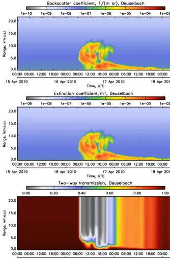
Figure 12.Time–height cross section of total backscatter coefficient, extinction coefficient, and two-way transmission, calculated by the forward model based on COSMO-ART output at Deuselbach station (western Germany). The vertical coordinates are given in kilometers above sea level (a.s.l.). The forward model used temperature, pressure, and volcanic ash particle data (no clouds, rain, fog, background aerosol, or other scattering objects). The two-way transmission is near 1 over clean-air conditions. Above ash layers, however, the two-way transmission has a value of only 5 %.
for each size class of COSMO-ART, and total lidar ratio can also be calculated. This was done, for example, at two time– height coordinates: the first coordinate points to model out-put from a coordinate inside the volcanic ash layer (Table 4).
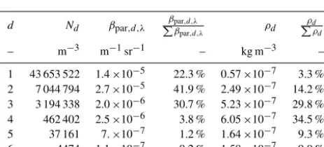
Table 4. Point-data extraction of COMSO-ART output at the Deuselbach ACL station; coordinate 1 is on 16 April 2010, 18:00 UTC, at a height of 1.9 km a.s.l. The individual backscatter coefficientβpar,d,λ, the contribution to the total backscatter coeffi-cientP
βpar,d,λ, the individual mass densityρd, and the contribu-tion to the total mass density P
ρd were calculated based on the model-predicted particle number densityNdof each size class d at this coordinate. Ash particles were calculated using a volumetric mass density of 2500 kg m−3. A non-linear relationship between the relative contribution to the total backscatter coefficient and the relative contribution to the transported mass of an ash size class can be observed: while the first three classes contribute 95 % of the to-tal backscatter coefficient, they carry only 78 % of the volcanic ash mass. This dependency on the laser wavelength can be seen as an advantage for multi-wavelength lidar systems.
d Nd βpar,d,λ
βpar,d,λ
Pβ
par,d,λ ρd
ρd
Pρ
d
– m−3 m−1sr−1 – kg m−3 –
1 43 653 522 1.4×10⁻⁵ 22.3 % 0.57×10⁻⁷ 3.3 %
2 7 044 794 2.7×10⁻⁵ 41.9 % 2.49×10⁻⁷ 14.2 %
3 3 194 338 2.0×10⁻⁶ 30.7 % 5.23×10⁻⁷ 29.8 %
4 462 402 2.5×10⁻⁶ 3.8 % 6.05×10⁻⁷ 34.5 %
5 37 161 7.×10−7 1.2 % 1.64×10⁻⁷ 9.3 %
6 4474 1.1×10⁻⁷ 0.2 % 1.58×10⁻⁷ 9.0 %
Table 5.The same as Table 4 but for coordinate 2 on 16 April 2010, 09:00 UTC, at a height of 1.5 km a.s.l. Even if class 4 carries only 27 % of the mass, it contributes 67 % of the total backscatter co-efficient. The inverse situation can be observed for the size class 6, which holds 73 % of the mass but contributes only 30 % of the backscatter coefficient at this coordinate.
d Nd βpar,d,λ
βpar,d,λ
Pβ
par,d,λ ρd
ρd
Pρ
d
– m−3 m−1sr−1 – kg m−3 –
1 93.0 30.7×10⁻¹² 0.2 % 0.01×10⁻⁹ 0.1 %
2 97.0 372.5×10⁻¹² 2.8 % 0.01×10⁻⁹ 0.1 %
3 1.0 6.2×10⁻¹² 0.1 % 0.01×10⁻⁹ 0.1 %
4 1700.0 9129.0×10−12 67.3 % 2.23×10⁻⁹ 27.1 %
5 0.5 10.2×10⁻¹² 0.1 % 0.01×10⁻⁹ 0.1 %
6 169.0 4018.8×10−12 29.6 % 5.97×10⁻⁹ 72.8 %
Regarding coordinate 1, the total backscatter coefficient is dominated by ash size classes 1, 2, and 3, while the signal contribution of classes 4, 5, and 6 is less than 5 % in total. The mass contribution is dominated by classes 3 and 4 while classes 2, 5, and 6 contribute 10 % of the total mass density. The total lidar ratio is 9.63 sr. Regarding coordinate 2, class 4 contributes about 68 % and class 6 about 30 % to the total backscatter coefficient. The mass contribution in coordinate 2 is also dominated by classes 4 and 6 but, in contrast to the backscatter coefficient, class 6 has a higher contribution to the total mass density than class 4. The total lidar ratio at this coordinate with predominately large particles is 46.53 sr.
General conclusions from this analysis about the relation-ship between backscattering and mass, depending on particle size and wavelength, require further investigation. For an ap-plication of the forward operator in this study, however, there are two aspects to be mentioned: first, the backscattering in-tensity inside the volcanic ash layer (coordinate 1) is predom-inantly dependent on classes 1, 2, and 3, whose backscatter cross sections are also overestimated by the forward operator due to the assumption of sphericity (see Fig. 11). The real values of the total lidar ratio may be a factor of 2–3 greater in certain cases (see Sect. 4.3). Second, the larger particles of classes 4, 5, and 6 carry a large portion of the mass but con-tribute only weakly to the total signal. This may be important information for the selection of future ACL networks. Prior studies confirm that even the systems operating at a relatively long wavelength of 1064 nm have a reduced sensitivity for giant and ultra-giant particles (Madonna et al., 2013). 5.3 Qualitative comparison
A comparison of ACL measurement and COSMO-ART sim-ulation with an applied forward operator at the Deuselbach ACL station in western Germany is shown in Fig. 13. The ash layer was clearly visible in the measured profiles with-out being affected by low-level or high-level clouds. Due to the inevitable instrumental noise and subsequent background subtraction, some data points become negative which is just a statistical effect but causes missing data in the log-scale plots. Volcanic ash plumes are clearly visible in both plots. Looking at the forward operator result, the ash layer begins to cross the ACL station between 06:00 and 12:00 UTC on 16 April 2010. The layer height decreases with time and partially entrains into the planetary boundary layer, where it persists even through the end of 17 April 2010. As both model and forward operator only represent volcanic ash and air molecules, the ash layers can be tracked within the plan-etary boundary layer. This is not possible using ACL mea-surements alone as the volcanic ash signal is tainted by other aerosol types. It is, however, difficult to determine unambigu-ously which ash layer structure observed by the ACL instru-ment can be related to corresponding structures simulated by the model. Regarding the thin volcanic ash layer which is measured by the ACL instrument at a height between 7 and 9 km a.s.l. on 16 April 2010, around 06:00 UTC, this feature could be equivalent to the model prediction of ash at a height of 6 km a.s.l. at 07:00 UTC. In this case, the model would have performed a rather precise prediction with only 1 h time lag and a 2 km vertical shift. But it is also possible that the predicted ash entrainment over the ACL station is equivalent to the ash-indicating ACL signals at around 12:00 UTC. In this case, the model prediction would be wrong by a time lag of about 6 h, which is insufficient for time-critical applica-tions.
Figure 13.Attenuated backscatter coefficient of ceilometer (top) and forward model (bottom) at Deuselbach station in Germany from 16 April 2010, 00:00 UTC, to 17 April 2010, 24:00 UTC, given in units of m−1sr−1. The ACL measurements in heights above 8 km a.s.l. are strongly affected by noise which limits the comparability of both data sets. A comparison of samples near the ground is limited by the missing overlap correction of ACL data and the lack of background aerosol prediction data. The ash layers in heights between 2 and 8 km a.s.l. allow for identifying similar and non-similar structures of measurement and forward-modeled COSMO-ART predictions of the Eyjafjallajökull ash. The maximum value of the (non-calibrated) ACL-measured attenuated backscatter coefficient is by about 1 order of magnitude lower than the attenuated backscatter coefficient from COSMO-ART prediction with BaLiFOp applied.
by both model and forward operator. There are, however, some scatterer fractions still missing in the present model runs for a comprehensive comparison: aerosol types other than volcanic ash such as anthropogenic emissions, mineral dust, soot, and pollen are not included, which leads to differ-ences, especially in the planetary boundary layer. It is hard to predict yet whether the strong ACL signal in the planetary boundary layer is related to background aerosol extinction or errors of the COSMO-ART prediction. To further investigate this problem, future studies with several types of aerosols in-corporated into the model are required.
5.4 Quantitative comparison
A major purpose of the backscatter lidar forward operator is also performing quantitative comparisons of measurement and model output data. Unfortunately, such a comparison is
of limited validity in this case study due to the unknown ACL calibration as noted in Sect. 3.2.
Outside the volcanic ash layer, the forward operator re-turns an attenuated backscatter coefficient value of 1× 10⁻⁷m−1sr−1, which is equal to the value of the ACL in-strument after calibration. This would be expected as both temperature and pressure are rather precisely determinable and the scattering properties of air are represented by the empirical equations which are used for the forward opera-tor. Thus, the selected calibration factor seems to be valid for this scenario.
is 20 times higher than the maximum value reported by the ACL (about 3.0×10⁻⁵m−1sr−1). Also, the forward-modeled attenuated backscatter coefficient shows strong tenuation due to the volcanic ash layer at 12 km a.s.l.: the at-tenuated backscatter coefficient is by about a factor of 10– 15 lower than at the same heights above clean-air condi-tions. Both findings indicate an overestimation of the model-predicted volcanic ash number density. However, an overes-timation of the ash concentration and preferring false alarms over misses are reasonable strategies for determining the haz-ardousness of volcanic ash particles using ash dispersion models.
6 Conclusions
A backscatter lidar model capable of calculating both the ex-tinction and backscatter coefficients was introduced. Detailed studies concerning the scattering properties of particles and molecules were performed. Instead of assuming a lidar ratio for given particles, this forward operator allows for calculat-ing the scattercalculat-ing properties even for mixtures of different particle types. Data of a COSMO-ART ash-dispersion sim-ulation for the Eyjafjallajökull eruption in 2010 were used to run the forward operator and perform both qualitative and quantitative comparisons between the output of the forward operator and measurement data of an automated ceilometer lidar (ACL) system. A major challenge for setting up the for-ward operator for a given scenario is the calculation of the effective extinction cross sectionσext,Rd,k,λand the effective differential backscatter cross sectionσbsc,Rd,k,λof all model-represented particle size and type classes.
The atmospheric gas mixture was treated as a uniform mixture ofatmospheric gasand empirical scattering formu-las were used to calculate its optical cross sections for the ACL laser wavelength. From the model-predicted values of temperature and pressure, the molecule number density and finally the molecule extinction and backscatter coefficients were calculated.
For particle scattering, the ranges of particle sizes were selected according to the volcanic ash classes used by COSMO-ART (six monodisperse classes with diameters of 1, 3, 5, 10, 15, and 30 µm). The range of considered refrac-tive indices were adapted according to in situ measurements of Schumann et al. (2011).
Due to uncertain refractive indices and shapes of the vol-canic ash, sensitivity studies have been performed to analyze the impact of different particle types and shapes on the effec-tive extinction and backscatter cross section and the pure li-dar ratio. While the extinction cross section was only weakly sensitive to variable refractive indices and particle shapes, the backscatter cross section was strongly sensitive to both. However, the sensitivities reduce significantly when apply-ing size-averagapply-ing algorithms. After averagapply-ing, the relative uncertainty of the effective backscatter cross section is up
to 280 % within the defined range of refractive indices. This study also indicates the dependency of the forward operator on precise information about the particle’s refractive index.
From the findings of Rocha-Lima et al. (2014), the aver-age aspect ratio of volcanic ash is known but there is no in-formation about a distribution function of particle shapes and real volcanic ash particles have an infinite variety of particle shapes. Consequently, the spherical shape was used as ref-erence even if the real volcanic ash particles are known to be fractal and complex shaped. Within a particle shape sen-sitivity study, the impact of the particle shape on extinction and backscatter cross sections was analyzed for 11 particle shapes (6 types of ellipsoids and 5 types of cylinders). The backscatter cross section spectrum of cylinders was differ-ent than the spectrum of ellipsoids and spheres. Sensitivity studies as presented here are mandatory for stepwise improv-ing the knowledge of scatterimprov-ing calculations related to lidar forward models. More detailed studies of scattering at non-spherical particles are thus mandatory to better represent the particle shape in the calculation of the effective backscatter cross section.
In the literature, we find measured lidar ratio values for volcanic ash between 40 sr and greater than 100 sr (Kokkalis et al., 2013; Mortier et al., 2013). This range of values could be observed within sensitivity studies of the pure lidar ratio (Sect. 4.3). From our analysis, the assumption of spherical particles results in a general underestimation of the lidar ratio except for size classes 1 and 4. Comparing the pure lidar ratio values of the first two size classes with the values reported by Gasteiger et al. (2011b), values of less than 20 sr seem to be plausible for these size parameters. The authors found a pure lidar ratio between 5 and 20 sr at size parameters between 5 and 15 (equivalent particle diameter at λ=1064 nm is 1.6 and 4.8 µm, respectively) even for irregularly shaped objects. The pure lidar ratio values output by the forward operator are thus realistic.
A time–height cross section comparison of ACL mea-surement and forward-modeled COSMO-ART output was shown. Similar structures were observed but some features were found at different times and heights. At the Deuselbach ACL station, some ash layer features were predicted quite precisely by the model, for example the time of arrival of the ash plume at about 06:00 UTC but vertically shifted by about 1.5 km. The ash plume intersection with the planetary bound-ary layer on 17 April 2010 at 03:00 UTC was simulated about 9 h too early on 16 April 2010 at 18:00 UTC. Fine structures of the ash layer were only observable in the simulation but not in the ACL data due to noise. Furthermore, the contribu-tion of individual classes to the total backscatter coefficient and to the total mass density for two sample cases were ana-lyzed.
The missing calibration coefficients of the ACL system re-quired the definition of a calibration constantη∗and to esti-mate its value comparing the ACL data with calibrated mea-surements at the same wavelength. Within quantitative com-parisons between ACL measurements and the forward opera-tor output, the molecule signal of ACL and forward operaopera-tor output were of the same order of magnitude which suggests that the selected calibration factor was reasonable.
A comparison of the measured and forward-modeled canic ash-attenuated backscatter coefficient inside the vol-canic ash plume led to the conclusion that the model-predicted ash concentration was too high which could po-tentially be resolved by reducing the model-predicted ash concentration manually by a given factor until the forward-modeled COSMO-ART predictions and ACL measurements are quantitatively similar. Such a reduction could be part of a simple particle data assimilation system helping to calibrate particle dispersion simulations before in situ measurements are available – assuming that the particles optical properties are known. It is therefore required to develop methods in the future which allow for fast determination of an aerosol type’s refractive index range, shape and aspect ratio.
As aerosol dispersion processes are directly coupled to vertical and horizontal movements in the atmosphere, a com-parison of forward-modeled and measured backscatter lidar profiles offers great potential for validating and improving the dynamic and thermodynamic components of an atmo-spheric chemistry model. For a model with variational data assimilation methods, the data assimilation system would se-lect the prediction variation which best fits the atmospheric state provided by lidar measurements, resulting in continuous adaptation of the model prediction to the real-world situation. The absolute values reported by the Raman lidar systems at a wavelength of 1064 nm agreed within the measurement uncertainties and expected natural differences in the sam-pled air mass with the results of the forward operator; see Sect. 5.2. This is quite remarkable given the large uncertain-ties of the ash data in the model (assumed emission rate of the volcano, atmospheric dynamics, dynamic of the mod-eled ash plume in the atmosphere including sedimentation)
and that there is no data assimilation regarding aerosol data at all yet. Further studies could focus on a comparison of forward-modeled lidar profiles and measurements from Ra-man or multi-wavelength lidar. In this context, the upcoming ESA satellite sensor EarthCARE with its HSRL is certainly of great interest.
There are, however, some error sources remaining: first, there are only molecules and the six volcanic ash classes represented while background aerosol is missing completely. Second, the ACL calibration is of limited precision. Third, the contribution to the attenuated backscatter coefficient of ash size classes 4, 5, and 6 is relatively low even though these classes carry a large portion of the mass. This relationship de-pends on the ACL’s wavelength. In our case of a wavelength of 1064 nm, the sensitivity is highest for particles with a di-ameter smaller than about 10 µm. Such results strengthen the importance of the joint use of observations and model out-put in combination with data assimilation in order to get a reliable description of the atmospheric state with respect to aerosol distributions and properties.
In conclusion, further investigation in scattering calcula-tions of non-spherical particles is recommended to get more realistic optical cross sections for the forward operator. A de-crease in uncertainties related to the forward operator can be achieved by refractive index measurements at the exact ACL wavelength. Refractive index measurements are a basic as-pect of the forward operator as the optical cross sections can only be calculated if the aerosols’ refractive index is known precisely. The model – and consequently the forward oper-ator – must represent more aerosol types, especially back-ground aerosols, mineral dust, sea salt, and soot, as missing extinction near the ground may cause the forward operator to overestimate the attenuated backscatter coefficient value from layers behind. Additionally, qualitatively more scatterer size classes are required to also represent the fine fraction and very large particles in the atmosphere. One approach for a better representation of the natural size spectrum of aerosols is the use of continuous number-size distributions which are aggregated from multiple distribution functions (“modal” ap-proach). This already includes the size averaging which is necessary for monodisperse size distributions. Furthermore, the model delivers exact information about the outer margins, i.e., the number density of the fine and the extreme coarse fraction which is currently not reproduced by model and for-ward operator in the selected case study.
Observation projects such as EARLINET (Pappalardo et al., 2014) and E-PROFILE (EUMETNET Profiling Programme) also focus on data quality improvements to meet the re-quirements of numerical weather prediction (NWP). In the spirit of these international activities, the creation of a central database for aerosol scattering properties and forward oper-ators would be desirable. Such a database can increase the development rate, flexibility, and applicability of current and future lidar forward operator implementations. Our operator is the basis also for other, more sophisticated operators and probably the best for backscatter lidar. The methodology and analysis presented here will be helpful for stepwise improv-ing our knowledge in how to deal with the important task of aerosol monitoring, modeling, and data assimilation in the future.
The uncertainties in both modeling and measurements will require sophisticated data assimilation algorithms not only for typical atmospheric variables but also for aerosol opti-cal properties. Also a very good first guess of model simu-lations with respect to aerosol particles will be necessary so that more sources, types, and sinks can be included. Within its priority project KENDA (Kilometer-Scale Ensemble Data Assimilation) the COSMO Consortium has developed an en-semble Kalman filter for data assimilation on the convec-tive scale. It has been used operationally by MeteoSwiss and DWD since March 2017. An advantage of the ensemble data assimilation system is that the assimilation can be carried out based on the pure forward operator, and that it is not neces-sary to calculate derivatives of the forward operator or the adjoint tangential model for carrying out data assimilation. Also, it naturally introduces model increments for all vari-ables where some dynamic covariance is observed from the underlying ensemble model runs. DWD aims to test the as-similation of ACL data into the COSMO-ART model based on BaLiFOp.
Data availability. The data for this paper can be made
available upon request from the authors Armin Geisinger ([email protected]), Andreas Behrendt ([email protected]), and Volker Wulfmeyer ([email protected]).
Competing interests. The authors declare that they have no conflict
of interest.
Acknowledgements. The present study was part of the research
project 50.0356/2012 funded by the German Federal Ministry of Transport and Digital Infrastructure (BMVI, prior BMVBS). We furthermore acknowledge the contributors to COSMO-ART, to the ceilometer network, to the IDL procedure mie_single, and to the T-matrix codes we used as a basis for our study. We are also thankful for helpful discussions with Cristina Charlton-Perez, Ina Mattis, Werner Thomas, and Frank Wagner. Furthermore, we would like
to acknowledge the travel support and very interesting discussions within the framework of the European COST (Cooperation in Science and Technology) action towards operational ground-based profiling with ceilometers, Doppler lidars, and microwave radiome-ters for improving weather forecasts (TOPROF).
Edited by: Andrew Sayer
Reviewed by: two anonymous referees
References
Ansmann, A., Tesche, M., Groß, S., Freudenthaler, V., Seifert, P., Hiebsch, A., Schmidt, J., Wandinger, U., Mattis, I., Müller, D., and Wiegner, M.: The 16 April 2010 major volcanic ash plume over central Europe: EARLINET lidar and AERONET photome-ter observations at Leipzig and Munich, Germany, Geophys. Res. Lett., 37, L13810, https://doi.org/10.1029/2010GL043809, 2010. Bangert, M., Nenes, A., Vogel, B., Vogel, H., Barahona, D., Kary-dis, V. A., Kumar, P., Kottmeier, C., and Blahak, U.: Sa-haran dust event impacts on cloud formation and radiation over Western Europe, Atmos. Chem. Phys., 12, 4045–4063, https://doi.org/10.5194/acp-12-4045-2012, 2012.
Banta, R. M., Brewer, W. A., Sandberg, S. P., and Hardesty, R. M.: Doppler Lidar–Based Wind-Profile Measurement Sys-tem for Offshore Wind-Energy and Other Marine Boundary Layer Applications, J. Appl. Meteorol. Clim., 51, 327–349, https://doi.org/10.1175/JAMC-D-11-040.1, 2012.
Behrendt, A., Nakamura, T., Onishi, M., Baumgart, R., and Tsuda, T.: Combined Raman lidar for the measurement of atmospheric temperature, water vapor, particle extinction coefficient, and particle backscatter coefficient, Appl. Opt., 41, 7657–7666, https://doi.org/10.1364/AO.41.007657, 2002.
Behrendt, A., Pal, S., Wulfmeyer, V., Álvaro M. Valdebenito B., and Lammel, G.: A novel approach for the characterization of transport and optical properties of aerosol particles near sources – Part I: Measurement of particle backscatter coefficient maps with a scanning UV lidar, Atmos. Environ., 45, 2795–2802, https://doi.org/10.1016/j.atmosenv.2011.02.061, 2011.
Benedetti, A. E. A.: Aerosol analysis and forecast in the European Centre for Medium-Range Weather Forecasts Integrated Forecast System: 2. Data assimilation, J. Geophys. Res., 114, D13205, https://doi.org/10.1029/2008JD011115, 2009.
Buchholtz, A.: Rayleigh-scattering calculations for the terrestrial at-mosphere, OSA Proc., 34, 2765–2773, 1995.
Chaboureau, J.-P., Richard, E., Pinty, J.-P., Flamant, C., Di Giro-lamo, P., Kiemle, C., Behrendt, A., Chepfer, H., Chiriaco, M., and Wulfmeyer, V.: Long-range transport of Saharan dust and its radiative impact on precipitation forecast: a case study during the Convective and Orographically-induced Precipita-tion Study (COPS), Q. J. Roy. Meteor. Soc., 137, 236–251, https://doi.org/10.1002/qj.719 2011.
Charlton-Perez, C. L., Cox, O., Ballard, S. P., and Klugmann, D.: A Forward model for atmospheric backscatter due to aerosols, clouds and rain, EMS Annual Meeting Abstracts, vol. 10 of EMS2013-313, 9–13 September 2013, Reading, UK, 2013. Chen, S., Zhao, C., Qian, Y., Leung, L. R., Huang, J., Huang,