Application of multifractal analysis to the study of SAR features and oil spills on the ocean surface

(1)

Nonlin. Processes Geophys., 21, 439–450, 2014 www.nonlin-processes-geophys.net/21/439/2014/ doi:10.5194/npg-21-439-2014

Nonlinear Processes

in Geophysics

Open Access

Application of multifractal analysis to the study of SAR features and

oil spills on the ocean surface

A. M. Tarquis1, A. Platonov2, A. Matulka2, J. Grau2, E. Sekula1,2, M. Diez3, and J. M. Redondo2

1_{CEIGRAM, E.T.S. de Ingenieros Agrónomos, U.P.M., Ciudad Universitaria s/n, 28040, Madrid, Spain} 2_{Departamento de Física Aplicada, Universitat Politècnica de Catalunya, EUETIB-CEIB, C/J.G. Salgado s/n,}

Campus Nord, Modul B4, 08034, Barcelona, Spain

3_{Ports de la Generalitat, Harbour of Vilanova i la Geltru, 08800, Barcelona, Spain} Correspondence to: J. M. Redondo ([email protected])

Received: 8 January 2011 – Revised: 21 November 2013 – Accepted: 14 January 2014 – Published: 28 March 2014

Abstract. The use of synthetic aperture radar (SAR) to vestigate the ocean surface provides a wealth of useful in-formation that is very seldom used to its full potential. Here we will discuss the application of multifractal techniques to detect oil spills and the dynamic state of the sea regarding turbulent diffusion. We present different techniques in order to relate the shape of the multifractal spectral functions and the maximum fractal dimension to the behaviour of the ocean surface. We compare eddy and sheared dominated flows with convective driven flows and discuss the different features and observation methods. We also compare the scaling of differ-ent oil spills detected by means of SAR images. Recdiffer-ent spills and weathered ones are selected and compared to investi-gate their behaviour in different spatial and temporal ranges. We calculate the partition function based on the grey inten-sity value of each SAR pixel deriving several types of multi-fractal spectra as a function of spill residence time estimated for each image. Image manipulations are seen to reduce the speckle noise and thus distinguish much better the texture of the oil spill images. The results are used to discuss how eddy diffusivity may be estimated and used in a description of the ocean surface using a simple turbulence kinematic simula-tion model to predict the shape of oil spills. Differences in the multifractal spectrum among SAR images may detect the slicks due to plankton and also provide information on the age of the oil spills, on the Lagrangian turbulent structure and on ocean surface diffusivity.

1 Introduction

Mixing and dilution processes in the ocean depend both on the local advection driven at the Rossby deformation radius as well as on the turbulent diffusion characteristics, with en-ergetic inputs at many different scales. The topology of trac-ers on the ocean surface (Carrillo et al., 2001; Diez et al., 2008) as well as the diffusion of pollutants clearly depend on the local characteristics of the turbulent cascades and on the characteristics of the whole energy and enstrophy spectra that in general will not be in local equilibrium in the sense of Kolmogorov (Kolmogorov, 1941, 1962). The dominant scale when stratification and rotation body forces are in equilib-rium in the ocean, local shear will transform slicks on the surface to align and follow the local flow, so the resulting pattern is much more varied than previously believed, and sets of eddies and spirals as shown by Munk (Munk et al., 2000; Platonov et al., 2008) clearly dominate the ocean be-haviour. The mixing processes at large-scale produce stirring, which maintains large gradients of the tracers, but in order to mix at molecular level in an irreversible fashion the energy has to cascade to the smallest internal scales, which are out-side the present-day range of observation (i.e. Kolmogorov or Batchelor scales; Redondo, 2002).

An important tool, fractal analysis, pioneered by Richardson and popularized by Mandelbrot (Mandelbrot, 1967; Feder, 1989; Turcotte, 1997), is motivated by the ap-pearance of multiple scales, which interact between them-selves in a highly non-linear fashion due to the appearance of turbulence. This is very common in environmental obser-vations, especially when the fluid regime leads to mixing

(2)

440 A. M. Tarquis et al.: SAR features and oil spills on the ocean surface

showing very complex patterns both temporally and spa-tially (Vassilicos, 1990; Vassilicos and Hunt, 1991; Redondo, 1990). The study of such effects demands new methods of image analysis and flow visualization, and these are in-creasingly provided by space agencies. The fractal and mul-tifractal analyses allow several well-defined measurements of the geometric level of complexity at different scales or ranges of scales (Benelli and Garzelli, 1999). Although the measurements we will present are purely geometrical in na-ture, often it is possible to relate these descriptors to impor-tant physical considerations of the flow or the pattern dis-tributions, or their statistics; some dynamical aspects can be measured, interpreted and thus predicted in a parameter space that can lead to very useful information (Redondo, 1990; Redondo and Linden, 1990; Mahjoub et al., 1998, 2000). Different fractal techniques can be used to calcu-late the fractal dimension or Kolmogorov’s capacity (Kol-mogorov, 1962, 1941) in different types of remote-sensing observations by means of satellite of the ocean (SAR), as has been shown by Platonov (2002), Platonov et al. (2001, 2002, 2008), Berrizi et al. (2004), Pérez-Marrero et al. (2006), and Pagnini et al. (2010), among others. The same type of anal-ysis may be performed in several other geophysical appli-cations, e.g. river flows, mountain heights, coastlines, and clouds (Hentschel and Procaccia, 1984; Turcotte, 1997). In all cases, when the dynamical multiscale features correspond to a high Reynolds number flow due to some tracers in the fluid or tensioactive substances (oil) in the ocean surface, the differences in complexity between different detected levels that reflect the physical dynamical conditions of the fluid en-vironment allow us a better understanding of the analysed flow and we may then relate the fractal measurements to the local energy spectrum, as defined in Kolmogorov theory in homogeneous turbulence (Linden et al., 1995).

Multifractals, also known as fractal measures, generalize the notion of fractals. Mandlebrot also worked on multifrac-tals in the 1970s and 1980s (Mandelbrot, 1988). Rather than being point sets, multifractals are measures (distributions) exhibiting a spectrum of fractal dimensions. Previous works on multifractal analysis of oil spills (Grau, 2005; Platonov et al., 2001, 2002, 2007, 2008) based on extracting a fractal dimension for a range of scales and for a single or a range of different grey intensities have been used to extract infor-mation from the ocean surface. In a similar way, it has been recognized that other features such as vortices or Langmuir-driven convergence lines on the ocean surface may reveal useful information. A traditional multifractal analysis has been applied (Platonov et al., 2007, 2008) to different fea-tures, but this work presents specific applications to investi-gate effective diffusion in the ocean and compares the differ-ent multifractal analysis applied to SAR images of oil spills as a topological or geometrical tool in order to differentiate them.

2 Self-similarity and turbulence cascades

Considering the periodT =1/f, the equation as a function of the spectral power S(f )=f−β may also be defined in scale L or in wavenumber space k=2π/L. If V (L) is a variance, calculated from the signal differences or from the shapes of the observed scalar field,Eis the Euclidian dimen-sion andDis the maximum fractal dimension (Redondo and Linden, 1996). The following relations are satisfied in local equilibrium turbulence:

S(f )≈LV≈L2H+1≈L2E+1−2D (1) H being Hausdorf’s dimension or co-dimension of the frac-tal dimensionH=E−D. Using this property, we may relate the spectral powerβtoDandEasβ=2E+ 1−2−D. So the fractal dimensionDunder the above-stated simple equi-librium hypothesis relates to the turbulence spectra as D=E+1−β

2 . (2)

This relationship is strictly valid for the maximum value of the fractal dimension; nevertheless, it is possible to evaluate the fractal dimension using box-counting algorithms for the whole range of scalar values of the analysed images, and this procedure is seen to provide useful geometrical information. In order to find a practical way of comparing images pro-duced by different physical mechanisms we will perform a fractal/multifractal analysis on SAR images of the ocean sur-face.

3 Multifractal analysis

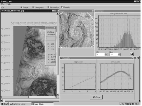
One of the promising techniques for automatic discrimina-tion of the oil spills is the calculadiscrimina-tion of fractal dimensions. Using the simple box-counting algorithm for SAR image analysis shows differences in the maximum fractal (box-counting) dimension of oil spills compared to other types of oceanic phenomena (Gade and Redondo, 1999). In Fig. 1 the results from applying the box-counting algorithm to a range of SAR intensities of a vortex seen by SAR are presented as the output of the Imacalc program (Grau, 2005). However, we can interpret SAR intensity values as a measure itself, and then study it as a statistical distribution applying multifractal methods (Grazzini et al., 2006). This can give us useful in-formation that one or two moments of the measurement only will not get, even if the underlying structure does not show self-similar or self-affine behaviour (Hentschel and Procac-cia, 1983; Halsey et al., 1986; Seuront et al., 1999).

For a monofractal object, the numberN of features of a certain size ε varies, as can be measured by counting the numberN of boxes needed to cover the object under inves-tigation for increasing box sizesεand estimating the slope of a log–log plot. For multifractal measurements, a probabi-lity distribution is measured using the box-counting method.

(3)

A. M. Tarquis et al.: SAR features and oil spills on the ocean surface 441

5

3 Multifractal analysis

One of the promising techniques for automatic discrimination of the oil spills is the calculation of

fractal dimensions. Using of the simple box-counting algorithm for SAR image analyzing shows

differences in the maximum fractal (box counting) dimension of oil spills compared to other types of

oceanic phenomena (Gade et al., 1998). In figure 1 the results from applying the box counting algorithm

to a range of SAR intensities of a vortex seen by SAR are presented as the output of Imacalc program

(Grau, 2005). However, we can interpret SAR intensities values as a measure itself, and then to study it as

a statistic distribution applying multifractal methods (Grazzini et al., 2006). This can give us useful

information that only with one or two moments of the measurement will not get, even if the underlying

structure does not show a self-similar or self-affine behaviour (Hentschel and Procaccia, 1983, Halsey et

al., 1986, Seuront et al., 1999).

Figure 1. Example of fractal calculations performed by Imacalc program on a SAR detected eddy grouping

the grey levels and extracting for each group the fractal dimension.

Fig. 1. Example of fractal calculations performed by the Imacalc

program on a SAR-detected eddy, grouping the grey levels and ex-tracting the fractal dimension for each group.

For every boxithe probability of “containing the object”, or in this application, the values of a certain SAR reflectivity, is also called the partition function (χ (q, δ)), which may be obtained for different q moments, which can vary following the equation

χ (q, δ)=

n(δ) X

i=1

µq_i(δ)=

n(δ) X

i=1

mq_i, (3)

wheremis the mass of the measure,qis the mass exponent, δis the length size of the box andn(δ)is the number of boxes in whichmi>0. Based on this, the mass exponent function

(τ (q))shows how the moments of the measure scale with the box size

τ (q)= lim

δ→0

logχ (q, δ) log(δ) =δlim→0

log<

n(δ) P

i=1

mq_i >

log(δ) , (4)

where<>represents the statistical moment of the measure mi defined on a group of non-overlappingn(ε)boxes of the

same size partitioning the area studied. The sum in the nu-merator of Eq. (4) is dominated by the highest values ofmi

forq >0, and by the lowest values ofmi forq <0 (Feder,

1989).

The singularity index (α)can be determined by Legendre transformation of theτ (q) curve (Evertsz and Mandelbrot, 1992) as

α(q)=dτ (q)

dq . (5)

The number of cells of sizeδwith the sameα,nα(δ), is

re-lated to the cell size asnα(δ)∝δ−f (α), wheref (α)is a

scal-ing exponent of the cells with commonα. Parameterf (α)

can be calculated as

f (α)=qα(q)−τ (q). (6)

A measure is multifractal when its multifractal spectrum (MFS), a graph ofαvs. f (α), exists and has the shape of an inverted parabola (Everetzs and Mandelbrot, 1992). MFS quantitatively characterizes the variability of the measure studied, with asymmetry to the right and left indicating dom-ination of small and large values respectively. The width of the MF (w)spectrum indicates overall variability.

3.1 Multifractal method

The study of the structured distribution in the space such that at any resolution the set is the union of similar subsets of the whole will indicate the same fractal dimension for every intensity value, but the scale factor in different parts of the set is not the same for most SAR images. If more than one dimension is needed, then the measure considered is charac-terized by the union of fractal sets, each one with a different fractal dimension.

With SAR images from the ocean surface we cannot rely strictly on theoretical limits for the calculation of the frac-tal, non-fractal or multifractal behaviour, because they have a finite size, and we have assigned a fixed range of values to the different SAR reflectivity intensities (from 0 to 255). The range of scale boundaries is defined by the image resolution, and we use numerical log/log fits (which tend to straighten any curve) to obtainτ (q). In order to cover the entire im-age, a rectangular box was used instead of a square one. For this reason, the bi-log fits were applied using the logarith-mic area values (lnδ2). The partition function was calculated fromq= −10 to+10, and regression fits used the maximum number of points with the condition thatR2had to be higher than 0.95.

3.2 Image manipulation

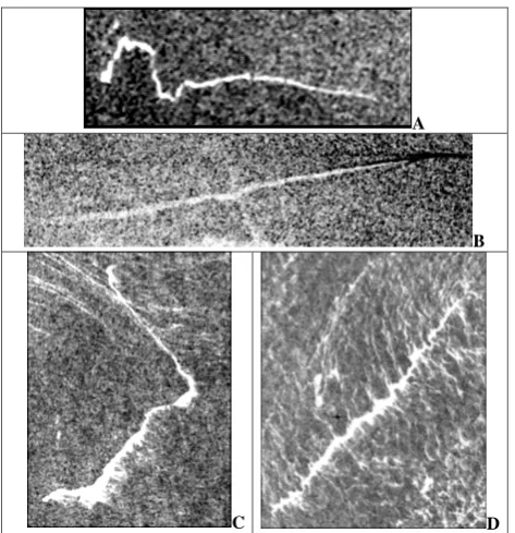
Satellite instruments are well adapted to monitor and there-fore to detect oil pollution, since they regularly produce im-ages of the sea surface including remote areas (Gade and Redondo, 1999; Anderson, 2002). Even several kinds of measurements have been tested; recently most attention has been given to the consideration of oil spills on synthetic aper-ture radar (SAR) images (Fingas and Brown, 2000). SAR seems to be one of the most suitable instruments for the detection of slicks, since slicks damp strongly short waves measured by SAR and oil spills appear as dark patches on the SAR image (see Figs. 1 and 2). SAR observations do not depend on weather (clouds) and sunshine, which allows the showing of illegal discharges that most frequently appear during night. SAR can also survey storm areas, provided the wind limits are appropriate, where accident risk is increased (Gade and Alpers, 1999).

(4)

442 A. M. Tarquis et al.: SAR features and oil spills on the ocean surface

8

Anderson, 2002). Even several kinds of measurements have been tested; recently main attention has been

given to consideration of oil spills on Synthetic Aperture Radar (SAR) images (Fingas and Brown, 2000).

SAR seems to be one of the most suitable instruments to the detection of slicks since slicks damp strongly

short waves measured by SAR and oil spills appear as a dark patch on the SAR image (see figure 1 and

2). SAR observations do not depend on weather (clouds) and sunshine, which allows showing illegal

discharges that most frequently appear during night. SAR can also survey storms areas, providing the

wind limits are appropiate, where accident risks are increased (Gade and Alpers, 1999).

A

B

C D

Figure 2. Several SAR images: for 21 January 1998 at Gibraltar (A), for 13 July 1997 at delta Ebro river

(B), for 24 August 1997 at Barcelona (C and D) showing illegal discharge of oil-polluted waters by ships.

The ship and its bow waves are clearly visible as white features at the beginning of the dark band in figure

B. Fresh discharges from moving ships are shown in figures A and B. Older weathered discharges are

shown in figures C and D.

Fig. 2. Several SAR images: for 21 January 1998 at Gibraltar (A),

for 13 July 1997 at the Ebro Delta (B), and for 24 August 1997 at Barcelona (C and D) showing illegal discharge of oil-polluted wa-ters by ships. The ship and its bow waves are clearly visible as white features at the beginning of the dark band in (B). Fresh discharges from moving ships are shown in (A) and (B). Older weathered dis-charges are shown in (C) and (D).

The constraints related to SAR measurements are of sev-eral kinds. Firstly, wind speed value has to be between 2–3 and 10–14 m s−1. Secondly, it is rather hard to distinguish oil spill from other phenomena which analogously to oil spills have negative radar contrast (look dark on SAR images) rel-ative the surrounding waters and commonly referred to as “look-alikes” (Jolly et al., 2000). The SAR images exhibited a large variation in natural features produced by winds, inter-nal waves, the bathymetric distribution, by thermal or solutal convection by rain, by plankton biological production, etc., as all of these produce variations in the sea surface rough-ness (Ming Li, 2000). The contrast between a spill and the surrounding water, and thus the probability of detecting pol-lution slicks, depends on the amount and type of oil spill as well as on environmental factors such as wind speed, wave height, SST, currents and current shift zones (Fingas et al., 2003).

Detecting the contrast patches also depends on the speckle noise, which is always present on the SAR images. Applica-tion of different filters to the radar data decreases the noise level and improves the feature detecting in the image. In this work, a Gaussian blur filter has been applied to reduce im-age noise and enhance imim-age structures at different scales. Mathematically, applying a Gaussian blur to an image is the

same as convolving the image with a Gaussian function; this is also known as a two-dimensional Weierstrass transform. The visual effect of this blurring technique is a smooth blur resembling that of viewing the image through a translucent screen (Gonzalez et al., 2004).

4 Results of oil spill analysis

After calculatingχ (q, δ)for the four original SAR images, lnχ (q, δ)was plotted against ln(δ2). In Fig. 3d, whereq is negative, two areas can be distinguished: one where the re-lationship between ln(δ2) and ln(χ (q, δ)) is linear and the other in which the value of ln(χ (q, δ)) is almost constant with respect to ln(δ2). In the case of Fig. 3c, these two ar-eas were not so marked, although the smallest area showed a different linear trend. At positive values ofq, the two differ-ent areas were not visible (see Fig. 3).

The presence of a plateau phase in ln(χ (q, δ))can be ex-plained by the resolution of these images. In certain small areas the scaling stops and the relationships among their val-ues remain approximately constant. After a certain critical area, however, a scaling pattern appears. This could be in-terpreted as the representative elementary area to study this scaling property. However, we have to consider that the parti-tion funcparti-tion for negative q is dominated by the smallest val-ues that in this case are the darker pixels that are precisely the ones that we have more interest in studying in the wider area range, as the image allows us. Trying to understand this effect better, the original images were inverted, so the darker pix-els were transformed into the lighter ones and with a higher numerical value. Thenχ (q, δ)was calculated again after sev-eral types of filters and manipulations of the images in order to show a clearer influence of the age of the spill (see Fig. 4). This time, the χ (q, δ) function followed a scaling be-haviour in the entireq range used in this study. However, in Fig. 5d the smallest scale forq=−8 to−10 still presents a slight difference in the linear trend, explained by the reso-lution of the image.

As well as applying this filter in the inverse images, the values of grey intensity were smoothed and the same multi-scale analysis was applied to the intensity values raised to a power of 3 (mi=m3i). Numerically, we passed from a range

of values of (0, 255) to (0, 2553), being the highest values related to the oil spills.

The effect of these transformations on the partition func-tion can be observed in Fig. 5, where the smallest area con-sidered in cases B, C and D shows a non-linear increase with respect to the rest of the scales at negative q values. This change is remarkable in case B, which is the image with the most distortion from the four considered. To calculateτ (q)in these last cases (after applying the image filter), the number of points for the regression fit, considering theR2value re-striction, was smaller in recent oil spills A and B figures. The results are shown in Figs. 5 and 6, where the main differences

(5)

A. M. Tarquis et al.: SAR features and oil spills on the ocean surface 443

Fig. 3. Partition function vs. area value in a bi-log plot: for 21 January 1998 at Gibraltar (A), for 13 July 1997 at the Ebro Delta (B), and for

24 August 1997 at Barcelona (C and D).

11

This time, the χ(q,δ) function followed a scaling behavior in all the q contemplated in this study. However, in figure 5D in the smallest scale for q=-8 to -10 still presents a slight difference in the linear

trend perfectly explained by the resolution of the image.

A

B

C D

Figure 4. Inverted SAR images after a Gaussian blur filter: for 21 January 1998 at Gibraltar (A), for 13 July 1997 at delta Ebro river (B), for 24 August 1997 at Barcelona (C and D) showing traces of oil-pollution produced from ships. (Redondo and Platonov 2009)

As well as applying this filter in the inverse images the values of grey intensity were smoothed,

the same multiscale analysis were applied to the intensity values raised to power of 3 ( 3

i i m

m = ). Numerically, we passed from a range values of (0, 255) to (0, 2553), being the higher values related to the

oil spills.

The effect of these transformations on the partition function can be observed in figure 5, where the

smallest area considered in case B, C and D shows a non linear increase respect to the rest of the scales at

negative q values. This change is remarkable in case B, which is the image with more distortion from the

four considered. To calculate τ(q)in these last cases (after applying the image filter) the number of points Fig. 4. Inverted SAR images after a Gaussian blur filter: for 21

Jan-uary 1998 at Gibraltar (A), for 13 July 1997 at the Ebro Delta (B), and for 24 August 1997 at Barcelona (C and D), showing traces of oil pollution produced by ships (Redondo and Platonov, 2009).

inτ (q)are found in the negativeqvalues, and these are more evident when the range of grey intensities increases.

The multifractal spectrum of these four images, doing an inversion of values with a Gaussian blur filter and increasing their grey value to a power of 3, give us a distinctive footprint

of the subtle topological differences between the more recent spill in image B and the older oil spills (images B and D). It is clear that the differences appear mostly in the negative part of theqvalues that correspond to the scaling behaviour of the areas with lower grey intensity, not belonging to the core of the oil spill, but to the region where most mixing takes place. We may also detect that even in the case of spill A, where the advection has distorted the spill due to large eddies, mixing has not been too strong.

An alternative way to calculate the multifractal spectra, which is defined as the limit towards the small scales, is to use a best fit centered at the intermediate scales in the interrogation region, which as seen in Fig. 7 would corre-spond to about half the size of the oil spill. The way in which these modified multifractal spectra are calculated is based on Eq. (2) for different groups of intensity values D(i). This procedure also provides relevant information that may be used to distinguish oil spills and natural slicks (Redondo and Platonov, 2009) or two-dimensional eddy type features and convective structures detected on the ocean surface. The dif-ferent self-similar image analysis tools have to be calibrated also considering the differences between the Lagrangian and Eulerian turbulent methods (Borgas, 1993; Sreenivasan and Meneveau, 1986).

5 Results of feature analysis and ocean diffusion

The ocean surface feature associated with the Rossby defor-mation radius is a typical vortex dipole structure, which is analysed with the ImaCalc program, as an example in Fig. 8 is marked as 6 in Fig. 9 (right); other vortex structures are

(6)

(A)

CHANGES NEEDED TO THE MANUSCRIPT npg-2010-123

FIGURE 5 (similar to 3) is missing and also the top of Figure 6

Figure 5 (in old typeset) should be figure 6 (Note CHANGE IN Figure CAPTION!)

Figure 5. Partition function versus area value in a bi-log plot for the inverted SAR

images after a Gaussian blur filter Simbols A-D correspond to image 4: for 21 January

1998 at Gibraltar (A), for 13 July 1997 at delta Ebro river (B), for 24 August 1997 at

Barcelona (C and D). -100 -50 0 50 100 150 200

0 2 4 6 8 10 12

ln(δ2)

lnχ (q, δ ) -10 -8 -6 -4 -2 0 2 4 6 8 10 -100 -50 0 50 100 150 200

0 2 4 6 8 10 12

ln(δ2)

ln χ (q, δ ) -10 -8 -6 -4 -2 0 2 4 6 8 10 -100 -50 0 50 100 150 200

0 2 4 6 8 10 12 ln(δ2)

lnχ (q, δ ) -10 -8 -6 -4 -2 0 2 4 6 8 10 -100 -50 0 50 100 150 200

0 2 4 6 8 10 12 ln(δ2

) ln χ (q, δ ) -10 -8 -6 -4 -2 0 2 4 6 8 10 (B)

CHANGES NEEDED TO THE MANUSCRIPT npg-2010-123

Barcelona (C and D). -100 -50 0 50 100 150 200

0 2 4 6 8 10 12

ln(δ2

) lnχ (q, δ ) -10 -8 -6 -4 -2 0 2 4 6 8 10 -100 -50 0 50 100 150 200

0 2 4 6 8 10 12

ln(δ2)

lnχ (q, δ ) -10 -8 -6 -4 -2 0 2 4 6 8 10 -100 -50 0 50 100 150 200

0 2 4 6 8 10 12 ln(δ2₎

lnχ (q, δ ) -10 -8 -6 -4 -2 0 2 4 6 8 10 -100 -50 0 50 100 150 200

0 2 4 6 8 10 12 ln(δ2)

ln χ (q, δ ) -10 -8 -6 -4 -2 0 2 4 6 8 10 (C)

CHANGES NEEDED TO THE MANUSCRIPT npg-2010-123

Barcelona (C and D).

-100 -50 0 50 100 150 200

0 2 4 6 8 10 12

ln(δ2)

lnχ (q, δ ) -10 -8 -6 -4 -2 0 2 4 6 8 10 -100 -50 0 50 100 150 200

0 2 4 6 8 10 12

ln(δ2)

lnχ (q, δ ) -10 -8 -6 -4 -2 0 2 4 6 8 10 -100 -50 0 50 100 150 200

0 2 4 6 8 10 12

ln(δ2)

lnχ (q, δ ) -10 -8 -6 -4 -2 0 2 4 6 8 10 -100 -50 0 50 100 150 200

0 2 4 6 8 10 12

ln(δ2)

ln χ (q, δ ) -10 -8 -6 -4 -2 0 2 4 6 8 10 (D)

CHANGES NEEDED TO THE MANUSCRIPT npg-2010-123

1998 at Gibraltar (A), for 13 July 1997 at delta Ebro river (B), for 24 August 1997 at

Barcelona (C and D).

-100 -50 0 50 100 150 200

0 2 4 6 8 10 12

ln(δ2)

lnχ (q, δ ) -10 -8 -6 -4 -2 0 2 4 6 8 10 -100 -50 0 50 100 150 200

0 2 4 6 8 10 12

ln(δ2)

lnχ (q, δ ) -10 -8 -6 -4 -2 0 2 4 6 8 10 -100 -50 0 50 100 150 200

0 2 4 6 8 10 12

ln(δ2₎

lnχ (q, δ ) -10 -8 -6 -4 -2 0 2 4 6 8 10 -100 -50 0 50 100 150 200

0 2 4 6 8 10 12

ln(δ2)

lnχ (q, δ ) -10 -8 -6 -4 -2 0 2 4 6 8 10

Fig. 5. Partition function versus area value in a bi-log plot for the inverted SAR images after a Gaussian blur filter Simbols A–D correspond

to image 4: for 21 January 1998 at Gibraltar (A), for 13 July 1997 at delta Ebro river (B), for 24 August 1997 at Barcelona (C and D).

Figure 6. Mass function (

τ

(q

)

(above) and multifractal spectrum (

α

vs.

f

(

α

)

(below) of inverted SAR images after a Gaussian blur filter with gray intensity (left column) and cubic of gray intensity (right column): for 21 January 1998 at Gibraltar (A), for 13 July 1997 at delta Ebro river (B), for 24 August 1997 at Barcelona (C and D).

FIGURE CAPTIONS SHOULD BE CHANGED 6 to 7, 7 to 8, 8 to 9, 9 to 10, 11 to 12 and 12 to

13.

THERE ARE 13 FIGURES IN TOTAL.

THE TEXT IS CORRECT

This addresses some of the Remarks from the editor and Typesetter

FINAL REMARKS:

CF1 - OK

-15 -13 -11 -9 -7 -5 -3 -1 1 3 5 7 9

-10 -8 -6 -4 -2 0 2 4 6 8 10 q τ (q) A B C D -19 -17 -15 -13 -11 -9 -7 -5 -3 -1 1 3 5 7 9

-10 -8 -6 -4 -2 0_q 2 4 6 8 10

τ (q ) A B C D 0.0 0.2 0.4 0.6 0.8 1.0

0.5 0.7 0.9 1.1 1.3 1.5 1.7 1.9

α f(α ) A B C D 0.0 0.2 0.4 0.6 0.8 1.0

0.5 0.7 0.9 1.1 1.3 1.5 1.7 1.9

α f(α ) A B C D

τ

(q

)

α

vs.

f

(

α

)

FIGURE CAPTIONS SHOULD BE CHANGED 6 to 7, 7 to 8, 8 to 9, 9 to 10, 11 to 12 and 12 to

13.

THE TEXT IS CORRECT

FINAL REMARKS:

CF1 - OK

-15 -13 -11 -9 -7 -5 -3 -1 1 3 5 7 9

-10 -8 -6 -4 -2 0 2 4 6 8 10 q τ (q) A B C D -19 -17 -15 -13 -11 -9 -7 -5 -3 -1 1 3 5 7 9

-10 -8 -6 -4 -2 0 2 4 6 8 10

q τ (q ) A B C D 0.0 0.2 0.4 0.6 0.8 1.0

0.5 0.7 0.9 1.1 1.3 1.5 1.7 1.9

α f(α ) A B C D 0.0 0.2 0.4 0.6 0.8 1.0

0.5 0.7 0.9 1.1 1.3 1.5 1.7 1.9

α f(α ) A B C D

τ

(q

)

α

vs.

f

(

α

)

FIGURE CAPTIONS SHOULD BE CHANGED 6 to 7, 7 to 8, 8 to 9, 9 to 10, 11 to 12 and 12 to

13.

THE TEXT IS CORRECT

FINAL REMARKS:

CF1 - OK

-15 -13 -11 -9 -7 -5 -3 -1 1 3 5 7 9

-10 -8 -6 -4 -2 0 2 4 6 8 10 q τ (q) A B C D -19 -17 -15 -13 -11 -9 -7 -5 -3 -1 1 3 5 7 9

-10 -8 -6 -4 -2 0_q 2 4 6 8 10

τ (q ) A B C D 0.0 0.2 0.4 0.6 0.8 1.0

0.5 0.7 0.9 1.1 1.3 1.5 1.7 1.9

α f(α ) A B C D 0.0 0.2 0.4 0.6 0.8 1.0

0.5 0.7 0.9 1.1 1.3 1.5 1.7 1.9

α f(α ) A B C D

τ

(

q

)

α

vs.

f

(

α

)

FIGURE CAPTIONS SHOULD BE CHANGED 6 to 7, 7 to 8, 8 to 9, 9 to 10, 11 to 12 and 12 to

13.

THE TEXT IS CORRECT

FINAL REMARKS:

CF1 - OK

-15 -13 -11 -9 -7 -5 -3 -1 1 3 5 7 9

-10 -8 -6 -4 -2 0 2 4 6 8 10 q τ (q) A B C D -19 -17 -15 -13 -11 -9 -7 -5 -3 -1 1 3 5 7 9

-10 -8 -6 -4 -2 0_q 2 4 6 8 10

τ (q ) A B C D 0.0 0.2 0.4 0.6 0.8 1.0

0.5 0.7 0.9 1.1 1.3 1.5 1.7 1.9

α f(α ) A B C D 0.0 0.2 0.4 0.6 0.8 1.0

0.5 0.7 0.9 1.1 1.3 1.5 1.7 1.9

α f(α ) A B C D

Fig. 6. Mass function (τ (q)) (above) and multifractal spectrum (αvs.f (α)) (below) of inverted SAR images after a Gaussian blur filter with gray intensity (left column) and cubic of gray intensity (right column): for 21 January 1998 at Gibraltar – A, for 13 July 1997 at delta Ebro river – B, for 24 August 1997 at Barcelona – C and D.

marked in Fig. 9 (left). The granular structure also detected is associated with heat-driven convection on the ocean surface. To compare the effects on scaling of the two physical pro-cesses stirring (mostly horizontally at large scales) the ocean surface, including waves and winds and generating

convec-tive cell structures by vertical overturning, it is important to distinguish the topology of the ocean surface eddies and other features such as Langmuir cells and Rayleigh–Benard cells.

(7)

A. M. Tarquis et al.: SAR features and oil spills on the ocean surfaceFIGURE 7 : 445

Fig. 7. Comparison of the multifractal spectrum (α vs.f (α)) of inverted SAR images after a Gaussian filter with grey intensity for spill (A), and for a smaller oil spill. The ImaCalc program may be downloaded from www.upc.edu.

The influence of waves on the dispersion coefficient has been poorly studied. Bezerra et al. (1998) and Diez et al. (2008) suggested that the contribution of surface waves af-fects the pollutant transport in two ways: by means of the mass flux and the increase in the turbulent processes. When a dye spot is released in the presence of waves, it can be seen that the spot moves in the wave-approaching direction, being the maximum velocity on the surface and decaying with depth. Besides, the waves contribute with turbulence, increasing the mixing processes. Correlations of the horizon-tal diffusion coefficient, the surface currents and the resultant vector of the oscillatory flow velocityumshow that the

ver-tical variation of the horizontal velocity component of the oscillatory flow (u’j)is another source of turbulent energy.

The effective contaminant transport is a combination of the individual effects of turbulence, waves and currents, which are driven by buoyancy and rotation. Zeidler (1976) showed for a series of experiments in the Baltic Sea that the exponent on the evolution of dye extension in time strongly depended on the distance from the coasty, so

σ2∝tn(y) (7)

with exponentn(y) varying between 2.3 and 1.2. This in-dicates anomalous diffusion, far from Richardson’s 4/3 law, where

K∝ε1/3l4/3. (8)

That in fully developed 3-D turbulence corresponds to a time dependence ofσ2∝t3.

Experiments also carried out by Zeidler (1976) in a wave flume showed a homogeneous dispersion in non-breaking waves with the absence of currents, i.e. the longitudinal

FIGURE 8

Fig. 8. Multifractal spectrum (αvs.f (α)) of a standard ERS-1 SAR image of a vortex dipole type of pattern near Barcelona. The image also shows some typical atmospheric-driven convective structures resulting in a complex patternD(i).

and lateral diffusion coefficients were constant (their vari-ances vary linearly with time), depending only on the non-dimensional parameterRwof waves (Rodriguez et al., 1995,

1999):

Rw=

a2 vT

sinh2π h L

−1/4

. (9)

This parameter could be considered as a Reynolds number, in whicha/T is the orbital velocity.

It can be seen that the coastal diffusion is larger in field conditions than those measured in the laboratory, increas-ing with time and the size of the dye spot (Zeidler, 1976; Bezerra et al., 1998; Rodriguez et al., 1999). So the wave dispersion is not linearly time dependent, probably due to the superposition of different effects such as diffusion generated by the oscillatory flow, bathometry-generated turbulence (by waves and currents) and shear dispersion due to the spatial gradients of the mean flux. Obviously the oil spills or tracers on the ocean surface grow during the diffusion process, so the concentration decreases. The irregularity of the acquired forms is due to the complex turbulent structure of the marine water movements, so its computation requires a specific nu-merical statistical process based on Einstein’s analogy with Brownian motion. Accepting a Gaussian spatial distribution of intensities and a lineal relationship between these and the concentrations, the dispersion coefficientKcan be estimated through a specific direction as a function of the dye blob (or oil spill) intensity varianceσ evolution:

K=1 2

dσ2

dt . (10)

(8)

446 A. M. Tarquis et al.: SAR features and oil spills on the ocean surface

15

Figure 9. Examples of Vortices detected in the ocean surface near Barcelona

The ocean surface feature, associated to the Rossby deformation radius is a typical vortex dipole structure which is analysed with program ImaCalc as an example in figure 8 is marked as 6 in figure 9(right), other vortex structures are marked in figure 9(left). The granular structure also detected is associated with heat driven convection in the ocean surface. To compare the effects on scaling of the two physical processes stirring (mostly horizontally at large scales) the ocean surface, including waves and winds and generating convective cell structures by vertical overturning, it is important to distinguish the topology of the ocean surface eddies and other features such as Langmuir cells and Rayleigh-Benard cells.

The influence of waves in the dispersion coefficient has been poorly studied. (Bezerra et al 1989,

Diez et al 2008) suggested that the contribution of surface waves affects the pollutants transport in two

ways: by means of the mass flux and increasing the turbulent processes. When a dye spot is released in

presence of waves, it can be seen that the spot moves in the wave approaching direction, being the

maximum velocity in the surface and decaying with depth. Besides, the waves contribute with turbulence,

increasing the mixing processes. Co-relations of the horizontal diffusion coefficient, the surface currents

and the resultant vector of the oscillatory flow velocity um show that the vertical variation of the

horizontal velocity component of the oscillatory flow (u’j) is another source of turbulent energy. The

effective contaminant transport is a combination of the individual effects of turbulence, waves and

currents, which are driven by buoyancy and rotation. Zeidler (1976) showed for a series of experiments in

the Baltic Sea that the exponent on the evolution of dye extension on the time strongly depended on the

distance from the coast y, so:

Fig. 9. Examples of vortices detected on the ocean surface near Barcelona.

Of course, this leads to K=σdσ

dt (11)

and Richardson’s 4/3 law is only applicable when the size of the blob is of the order of the integral length scale,σ ≈l, and then, as in 3-D flows,

u0∝ε1/3l1/3 (12)

K=lu0≈ε1/3l4/3. (13)

Image analysis of vortices in the ocean surface

Using the multi-fractal analysis of SAR images (Bunimovich et al., 1993; Jolly et al., 2000) we may detect a large variation in natural features produced by winds, internal waves, the bathymetric distribution, by thermal or solutal convection, by rain, etc., as all of these produce variations in the sea surface roughness.

The satellite-borne SAR is able to detect oceanic features with a range of scales as seen in Fig. 9, which shows sev-eral eddy structures in the NW Mediterranean area (Redondo and Platonov, 2009; Sekula and Redondo, 2008). The images show a wide range of values, if we suppose that the surface currents are responsible (at least partly) for the spatial distri-bution of the ocean roughness for two main reasons. First, the slope on both sides of an eddy is very different at producing radar backscatter from the side (as happens with ERS-1/2 and ENVISAT); the other reason is that the surface tensioactives, either natural or man-made, will be advected by the surface current lines and concentrated by Langmuir cells, so there may be a strong spatial relationship between the SAR inten-sity and the shear–vorticity distribution within the complex mesoscale ocean surface topology.

18

to Langmuir convergence lines). It is obvious that the dark features, being elongated and smoother have a smaller fractal dimension than the background area between the spiral structures. But the appearance of a linear increase is not clear. The fact that convective structures take place in all the images and the structures are marked both by darker (meaning a smooth surface) and white (rougher sea surface areas) explains that at a wider range the maximum fractal dimension (D1) is about the same (1.55) for convective cells.

Figure 10 - D(i) multifractal spectra for several vortex/convective structures in figure 9 Fig. 10. D(i) multifractal spectra for several vortex/convective structures in Fig. 9.

In SAR images, where convective cells are formed on the ocean surface, it is interesting to compare the multifractal appearance of the different signatures, and this is shown in Fig. 10 for the examples indicated in Fig. 9. The only quite different fractal structure is the bottom-right one correspond-ing to the convective cells, where a clear plateau of a con-stant value of the maximum fractal dimension indicates that this measure is the same for the different intensity values of the SAR images. On the other hand, the vortical-dominated structures exhibit a slightly higher fractal value (1.7) for the higher SAR reflectivity (white) and a linear increase from the darker features (lines that indicate the vertical structure, mostly due to Langmuir convergence lines). It is obvious that the dark features, being elongated and smoother, have a smaller fractal dimension than the background area between the spiral structures, but the appearance of a linear increase is not clear. The fact that convective structures appear on all the images and that the structures are marked both by darker (meaning a smooth surface) and white (rougher sea surface

(9)

A. M. Tarquis et al.: SAR features and oil spills on the ocean surface 447

FIGURE 11

11 a) 11 b)

11 c) 11 d)

Fig. 11. SAR images of the natural slick (a) of an oil spill, (b) of a

weather front line, and (c) of a combination of oil spills and look-alike weather reflections from the atmosphere (d).

20

0 0.4 0.8 1.2

Normalized SAR intensity i/io 1

1.2 1.4 1.6

Fr

ac

ta

l d

im

en

sio

n

D(

i)

Figure 12. The comparison of the multifractal spectrum of the images (a) and (b) shown in figure 11, (a)Natural slick (squares) and (b) released recent but weathered oil spill (circles).

Figure 12 compares the recent oil spill (Figure 11b) as circles with a natural slick that has adapted to the

natural similarity of a fully turbulent environment, indicated as squares that corresponds to image 11 a).

The use of the multifractal analisis has been shown to provide more information about the different types

of generation and of the complexity of the interacting scales in different physical conditions. When

comparing SAR images of recent oil spills with weathered natural slicks there are two distinct differences

between both SAR images, the natural slicks have adapted to the background turbulent flow and passive

tracers show a parabolic shape of the multifractal spectrum with a maximum near the ambient intensity.

The recent oil spills have also lower maximum fractal dimension values for a range of medium intensity

values, but they show a higher fractal value of 1.1-1.3 for the very low SAR reflectivity values, indicating

the actual extension of the oil spill. In time, as the oil spill is diluted and advects in a similar way as a

natural slick, both plots tend to converge. All of the techniques shows complement each other but the

different physical proceses that force the turbulence cascades both 2D (inverse) and 3D (direct) not only

intermittently (Mahjoub et al. 1998) but in a non-local fashion so that neither the spectral slope nor the

multifractal spectra behave in a simple way, see for example the D(i) multifractal spectra for a river

plume in (Sekula and Redondo 2008).

To understand the evolution of a tensioactive or oil spill modeled as a tracer, it is possible to use a Kinematic Simulation (KS) Model of turbulence in a two dimensional type of cascade, This model is described in Castilla et al.(2007) and Diez et al.(2008), in order to quantify the evolution of an oil spill in the ocean surface here it is just necessary to present the results of the monotonic growth of the maximum fractal dimension of a

Fig. 12. The comparison of the multifractal spectrum of the images (a) and (b) shown in Fig. 11. (a) Natural slick (squares) and (b)

recently released but weathered oil spill (circles).

areas) explains why at a wider range the maximum fractal dimension (D1) is about the same (1.55) for convective cells. Figure 11 shows a well-defined oil spill that has been a relatively short time on the ocean surface A (b) as well as a natural slick that has had a distributed generation process and developed into a parabolic multifractal type (a), which is typical of turbulent processes (Gade and Redondo, 1999). Figure 11c shows the SAR effect of a front or squall line while Fig. 11d shows some internal waves beside an oil spill. Figure 12 compares the recent oil spill (Fig. 11b) as cir-cles with a natural slick that has adapted to the natural sim-ilarity of a fully turbulent environment, indicated as squares that correspond to Fig. 11a. The use of multifractal analysis has been shown to provide more information about the dif-ferent types of generation and the complexity of the

interact-21

marked line of passive tracer mimicking an oil spill as it evolves in time. The results of a set of numerical experiments are shown in figure 13 where the maximum value of the fractal dimension of an oil spill in rough weather is simulated, see Apendix 1 for details of the synthetic simulation model of turbulence diffusing an oil spill, more information may be found in ( Nicoleau et al 2012).

It has been demonstrated that it is necessary to use a non/dimensional time normalized with the local energy dissipation in a similar way as the Damkholer reactive number that characterizes the level of local turbulence in the ocean surface

Figure 13. The evolution of the maximum fractal dimension of the K.S. oil spill shapes released in a 2D turbulent model of the ocean surface. Time is normalized by the Damkholer number.

6 Conclusions

The use of the multifractal analyses has been shown to provide more information about the

different types of generation and of the complexity of the interacting scales in different physical

conditions. We confirm the usefullness of scaling information provided by a knowledge of the

multifractal spectral functions, both centered at intermediate scales and calculated in the usual way as a

limit to the smallest scales, normally limited by the pixel size.

0 0.1 0.2 0.3 0.4 0.5 0.6 0.7 0.8 0.9 1 1.1 1.2 t/Td

1 1.2 1.4 1.6

F

ra

ct

a

l D

im

e

n

si

o

n

Fig. 13. The evolution of the maximum fractal dimension of the

K. S. oil spill shapes released in a 2-D turbulent model of the ocean surface. Time is normalized by the Damkholer number.

ing scales in different physical conditions. When comparing SAR images of recent oil spills with weathered natural slicks there are two distinct differences between both SAR images: the natural slicks have adapted to the background turbulent flow and passive tracers show a parabolic shape of the mul-tifractal spectrum, with a maximum near the ambient inten-sity. The recent oil spills also have lower maximum fractal dimension values for a range of medium intensity values, but they show a higher fractal value of 1.1–1.3 for the very low SAR reflectivity values, indicating the actual extent of the oil spill. In time, as the oil spill is diluted and advects in a similar way as a natural slick, both plots tend to converge. All of the techniques shown complement each other, but the different physical processes force the turbulence cascades both 2-D (inverse) and 3-D (direct) not only intermittently (Mahjoub et al., 1998), but in a non-local fashion, so that neither the spectral slope nor the multifractal spectra behaves in a sim-ple way; see for examsim-ple theD(i)multifractal spectra for a river plume in Sekula and Redondo (2008).

To understand the evolution of a tensioactive or oil spill modelled as a tracer, it is possible to use a kinematic simu-lation (KS) model of turbulence in a two-dimensional type of cascade. This model is described in Castilla et al. (2007) and Diez et al. (2008). In order to quantify the evolution of an oil spill on the ocean surface here it is just necessary to present the results of the monotonic growth of the maximum fractal dimension of a marked line of passive tracer mimick-ing an oil spill as it evolves in time. The results of a set of numerical experiments are shown in Fig. 13, where the max-imum value of the fractal dimension of an oil spill in rough weather is simulated; see Appendix 1 for details of the syn-thetic simulation model of turbulence diffusing an oil spill; more information may be found in Nicoleau et al. (2012).

(10)

It has been demonstrated that it is necessary to use a non/dimensional time normalized with the local energy dis-sipation in a similar way as the Damkholer reactive number that characterizes the level of local turbulence on the ocean surface.

6 Conclusions

The use of the multifractal analyses has been shown to pro-vide more information about the different types of genera-tion and the complexity of the interacting scales in different physical conditions. We confirm the usefulness of scaling in-formation and knowledge of the multifractal spectral func-tions, both centered at intermediate scales and calculated in the usual way as a limit to the smallest scales, normally lim-ited by the pixel size.

The curvature of the mass functions has no unique rela-tionship with a single physical parameter, but it is clearly influenced by the topological effects produced by a longer dilution in time. It has been demonstrated that it is necessary to use a non/dimensional time normalized with the local en-ergy dissipation in a similar way as the Damkholer reactive number. The oil spills are more convoluted in time and their maximum fractal dimension grows towards a fully turbulent flow. They also approach a parabolic multifractal spectrum shape in time.

When comparing SAR images of recent oil spills with older ones, there are distinct differences between both SAR images. The inverted and blurred images of recent oil spills have a wider range ofα values (Hölder exponent), mean-while the older oil spills show a narrower range. In time, as the oil spill is diluted and eventually advects in a similar way as a natural slick, one plot (recent spill) tends to converge to the other one (older spills and slicks). The Lagrangian turbulence effects as well as the wall effects on turbulence (Sreenvassan and Meneveau, 1986) show the role of inter-mittency (kurtosis) in the fractal structure, so relationship (2) needs to be generalized for the different parts of the scale-to-scale cascade processes that disperse oil and other tracers on the ocean surface. One such possibility is to relate local diffusion to the second-order structure function that depends on the maximum fractal dimension.

Appendix A

There are many ways to simulate fluid flow, but when this is turbulent, these simulations become complicated, expensive and inaccurate at a large Reynolds number. Using a kine-matic simulation (KS) model, we have compared some pre-dictive results on the tracer shape evolution with examples of real detected oil spills and field measurements. We present some simple theoretical and numerical bases needed to sim-ulate the behaviour of oil spills (or tracer particles) in a turbu-lent flow in a simple and efficient way using measured

veloc-ity fields, which may be updated with the latest output from dedicated environmental atmosphere (wind) and ocean cur-rents or wave-nested models. There is a strong dependence of horizontal eddy diffusivities on the wave height and the local wind. Some of these results have been published in Bezerra et al. (1998). Both effects are important and give sev-eral decades of variation in eddy diffusivities measured near the coastline (between 0.0001 and 2 m2s−1).

A series of kinematic simulations have been used to study the fractal dimension of a marked set of tracers and their dif-fusion in a homogeneous, quasi 2-D non-stratified flow that models the ocean surface. Detailed results on the method and the structure of the 2-D turbulence are also described in Castilla et al. (2007) and Nicolleau et al. (2011).

The velocity calculation at any point x at a determined instanttis made with the expression

v=

N X

n=0

[Ansin(κnx+ωnt )+Bncos(κnx+ωnt )], (A1)

wherevn=knωn is the turnover velocity of the eddy with

scaleln, and is related to the energy through

ωn=λ q

κ_ij3E(κn) (A2)

whereλis a parameter which indicates the turbulence sta-tionarity degree. The vectorsκnhave random direction and

sense, and their moduli depend on the discretization in phase space.

The vectorsAn andBn also have random direction and

sense, but they must be normal toκn.

Its modulus is also random, but with Gaussian distribution centered at 0 and with variance equal to the level of energy E(ln)exhibited by the spectrum.

The simulation is then controlled by the integral and Kol-mogorov scales, the molecular viscosity of fluid,v, and the spectrum shape within the inertial subrange. From a numer-ical point of view, we divide the wavenumber inertial range into N intervals, which can be calculated following a geomet-ric progression in order to put, more or less, a comparable realistic energy at each scale.

When we have calculated the velocity field, we trace a suf-ficiently high number of particles randomly distributed, with a determined initial standard deviation, and we study its tem-poral development calculating the fractal dimension.

Our particles are passive tracers. The movement equations are

dxp

dt =v(xp, t ), (A3)

wherexpthe particle position andv(xp,t) is the fluid

veloc-ity.

An important characteristic of KS is that we do not need a grid. We can calculate fluid velocity at any position and time. To integrate Eqs. (A1) and (A3), we have used a fourth-order Runge–Kutta scheme with a fixed time step. The time step

(11)

A. M. Tarquis et al.: SAR features and oil spills on the ocean surface 449

is a fraction of the characteristic turnover time of the small-est eddies given by Kolmogorov (1941), and over a range of scales where diffusivity behaves according to the 4/3 law (Richardson, 1929).

Intuitively, we expect the size of the cloud to grow rapidly when it is of a size embedded in the inertial range, and then to slow down when it reaches and exceeds the integral scale. LetLbe the particle set size. If its value is of the order of, or smaller than, the turbulence integral scale, the eddies mod-ify its value in a sizeable way. However, ifLis much bigger than the integral scale, this modification does not much af-fect the global growth of the cloud of tracers simulating the oil spill.

The eddy diffusivities in the ocean exhibit large variation and show marked anisotropy. Not only are horizontal values much larger than vertical ones, but there is a strong depen-dence on the spatial extent of the tracer dye or pollutant and at larger scales the topology of the basic flow is very impor-tant. In the case of oil spills, these are strongly influenced by the buoyancy and horizontal diffusion depends on ambient factors such as wave activity, wind and currents. The non-dimensional time used, Td, may be derived through dimen-sional analysis from the integral length scale and the turbu-lence dissipation.

Acknowledgements. This work was funded by the Ministerio de

Ciencia, Tecnologia e Innovacion of Spain and the Universitat Politècnica de Catalunya (ESP2005-07551, FTN-2001-2220). The authors also acknowledge ENV4-CT96-0334 and ISTC-1481 Eu-ropean Union projects for support and the ESA (AO-ID C1P.2240) for the SAR images provided. Thanks are also due to ERCOFTAC (PELNoT, SIG 14). We thank the editor and referees for assisting in evaluating and improving this paper.

Edited by: I. Tchiguirinskaia

Reviewed by: three anonymous referees

References

Anderson, A. G.: The Media Politics of Oil Spills, Spill Sci. Tech-nol. B., 7, 7–15, 2002.

Benelli, G. and Garzelli, A.: Oil-spills detection in SAR images by fractal dimension estimation, in: Geoscience and Remote Sens-ing Symposium, IGARSS ’99 ProceedSens-ings, IEEE 1999 Interna-tional, 1, 218–220, 1999.

Berrizi, F., Dalle Mese, E., and Martorella, M.:, A sea surface fractal model for ocean remote sensing, Int. J. Remote Sens., 25, 1265– 1270, 2004.

Bezerra, M. O., Diez, M., Medeiros, C., Rodriguez, A., Bahia, E., Sanchez Arcilla, A., and Redondo, J. M.: Study on the influence of waves on coastal diffusion using image analysis, Appl. Sci. Res., 59, 127–142, 1998.

Borgas, M. S.: The Multifractal Lagrangian Nature of Turbulence, Philos. T. R. Soc. A. , 342, 1665, 379–411, 1993.

Bunimovich, L. A., Ostrovsky, A. G., and Umatani, S.: Observa-tions of the fractal properties of the Japan Sea surface tempera-ture patterns, Int. J. Remote Sens., 14, 2185–2201, 1993. Carrillo, A., Sanchez, M. A., Platonov, A., and Redondo, J. M.:

Coastal and interfacial mixing; Laboratory experiments and satellite observations, Phys. Chem. Earth. B, 26, 305–311, 2001. Castilla, R., Redondo, J. M., Gámez-Montero, P. J., and Babiano, A.: Particle dispersion processes in two-dimensional turbulence: a comparison with 2-D kinematic simulation, Nonlin. Processes Geophys., 14, 139–151, doi:10.5194/npg-14-139-2007, 2007. Diez, M., Bezerra, M. O., Mosso, C., Castilla, R., and Redondo,

J. M.: Experimental measurements and difusión in harbor and coastal zones, Il Nouvo Cimento C, 31, 5/6, 843–859, 2008. Evertsz, C. J. G. and Mandelbrot, B. B.: Multifractal measures, in:

Chaos and Fractals: New Frontiers of Science, edited by: Peitgen, H., Jurgens, H., and Saupe, D., Springer-Verlag, NY, 921–953, 1992.

Feder, J.: Fractals. Plenum Press, New York, 296 pp., 1989. Fingas, M. and Brown, C.: A Review of the Status of Advanced

Technologies for the Detection of Oil in and with Ice, Spill Sci. Technol. B., 6, 295–302, 2000.

Fingas, M., Fieldhouse, B., and Wang, Z.: The Long Term Weath-ering of Water-in-Oil Emulsions, Spill Sci. Technol. B., 8, 137– 143, 2003.

Gade, M. and Alper, W.: Using ERS-2 SAR images for routine ob-servation of marine pollution in European coastal waters, Sci. Total Environ., 237/238, 441–448, 1999.

Gade, M. and Redondo, J. M.: Marine pollution in European coastal waters monitored by the ERS-2 SAR: a comprehensive statistical analysis, IGARSS 99, Hamburg, III, 1637–1639, 308–312, 1999. Gonzalez, R. C., Woods, R. E., and Eddins, S. L.: Digital Image Pro-cessing using MATLAB, Pearson Prentice Hall, 597 pp., 2004. Grau, J.: Analysis of the Meteosat images sequences using the

dig-ital processing method, Ph.D. thesis, UPC, Barcelona, 2005. Grazzini, J., Turiel, A., Hussein Yahiac, and Herlin, I.: A

multi-fractal approach for extracting relevant textural areas in satellite meteorological images, Environ. Modell. Softw., 22, 323–334, 2006.

Halsey, T. C., Jensen, M. H., Kadanoff, L. P., Procaccia, I., and Shraiman, B. I.: Fractal Measures and their Singularities – the Characterization of Strange Sets, Phys. Rev. A, 33, 1141–1151, 1986.

Hentschel, H. G. E. and Procaccia, I.: Fractal nature of turbulence as manifested in turbulent diffusion, Phys. Rev. A, 27, 1266–1269, 1983.

Hentschel, H. G. E. and Procaccia, I.: Relative diffusion in turbulent media: The fractal dimension of clouds, Phys. Rev. A, 29, 1461– 1470, 1984.

Jolly, G. W., Mangin, A., Cauneau, F., Calatuyud, M., Barale, V., Snaith, H. M., Rud, O., Ishii, M. Gade, M., Redondo, J. M., and Platonov, A.: The Clean Seas Project Final Report DG XII/D of the European Commission under contract ENV4-CT96-0334, Brussels, 2000.

Kolmogorov, A. N.: The Local structure of turbulence in incom-pressible viscous fluid at very large Reynolds numbers, C. R. Acad. Sci. USSR, 30, 301, 1941.

Kolmogorov, A. N.: A refinement of previous hypotheses concern-ing the local structure of turbulence in a viscous incompressible fluid at high Reynolds number, J. Fluid Mech., 13, 82–85, 1962.

(12)

450 A. M. Tarquis et al.: SAR features and oil spills on the ocean surface

Linden, P. F., Boubnov, B. M., and Dalziel, S. B.: Source-sink tur-bulence in a rotating, stratified fluid, J. Fluid Mech., 298, 81-112, 1995.

Mahjoub, O. B. Redondo, J. M., and Babiano, A.: Structure func-tions in complex flows, Appl. Sci. Res., 59, 299–313, 1998. Mandelbrot, B. B.: How long is the coast of Britain? Statistical

self-similarity and fractional dimension, Science, 156, 636–638, 1967.

Mandelbrot, B. B.: An introduction to multifractal distribution func-tions, in: Random Fluctuations and Pattern Growth: Experiments and Models, Springer Netherlands, 279–291, 1988.

Ming Li: Estimating Horizontal Dispersion of Floating Particles in Wind-driven Upper Ocean, Spill Sci. Technol. B., 6, 255–261, 2000.

Munk, W., Armi, L., Fischer, K., and Zachariasen, F.: Spirals on the Sea, P. Roy. Soc. Lond. A-Mat., 456, 1217–1280, 2000. Nicolleau, F. C., Cambon, C., Redondo, J. M., Vassilicos, J. C.,

Reeks, M., and Novakowski, A. F. (Eds): New approaches in modeling multiphase flows and dispersion in turbulence, frac-tal methods and synthetic turbulence, ERCOFTAC Series 18, Springer Academic Publishers, 2011.

Pagnini, G., Strada, S., Maurizi, A., and Tampieri, F.: La-grangian stochastic modeling for oil spills turbulent dispersion on ocean surface, Commun. Appl. Indust. Mathe., 1, 185–204, doi:10.1685/2010CAIM480, 2010.

Pérez-Marrero, J., Maroto, L., Llinás, O., Rueda, M. J., Tejera, A., Godoy, J., and Barrera, C.: Integración de observaciones remo-tas y modelos hidrodinámicos para el estudio de la dispersión de contaminantes en el mar, Revista de Teledetección, Special Vol-ume June 2006, 60–64, 2006 (in Spanish).

Platonov, A.: Application of the SAR images to the investigations of marine pollution and NW Mediterranean waters’ dynamics, Ph.D. thesis, available at: http://www.tdx.cbuc.es, 2002 (in Span-ish).

Platonov, A., Redondo, J. M., and Grau, J.: Water wash spill pol-lution danger in the NW Mediterranean: statistical analysis of two- year satellite observations, Maritime Transport 2001, De-partment of Nautical Science and Engineering de la UPC and Grup Artyplan-Artympres, S.A. Barcelona, 1., 325–334, 2001. Platonov, A., Grau, J., and Redondo, J. M.: The structure and

dif-fusion of the oil spills and slicks in the ocean, Proceedings of the Fluxed and Structures in the Fluids International Conference, RAS, Moscow, 176–183, 2002.

Platonov, A., Tarquis, A., Sekula, E., and Redondo, J. M.: SAR observations of vortical structures and turbulence in the ocean; Models, Experiments and Computations in Turbulence, edited by: Castilla, R., Oñate, E., and Redondo, J. M., CIMNE, Barcelona, 195–230, 2007.

Platonov, A., Carrillo, A., Matulka, A., Sekula, E. Grau, J., Redondo, J. M., and Tarquis, A.: Multifractal observations of ed-dies, oil spills and natural slicks in the ocean surface, Il Nuovo Cimento C, Vol. 31, 5/6, 861–880, 2008.

Redondo, J. M.: The structure of density interfaces, PhD. thesis, University of Cambridge, UK, 1990.

Redondo, J. M.: Mixing efficiency of different kinds of turbulent processes and instabilities, Applications to the environment, Tur-bulent Mixing in Geophysical Flows, CIMNE, Barcelona, edited by: Linden, P. F. and Redondo, J. M., 131–157, 2002.

Redondo, J. M. and Linden, P. F.: Geometrical Observations of Tur-bulent Density Interfaces, in: Mathematics and computation of deforming surfaces , edited by: Dritshel, D. G. and Perkings, R. J., Clarendon Press, Oxford, IMA, 56, 222–248, 1996.

Redondo, J. M. and Platonov, A. K.: Self-similar distribution of oil spills in European coastal waters, Environ. Res. Lett., 4, p. 014008, doi:10.1088/1748-9326/4/1/014008, 2009.

Redondo, J., Rodriguez, A., Bahia, E., Falqués, A., Gracia, V., Sánchez Arcilla, A., and Stive, M. J. F.: Image Analysis of Surf-Zone Hydrodynamics, Coastal Dynamics’94, ASCE, 350–365, 1994.

Redondo, J. M., Grau, J., Platonov, A., and Garzon, G.: Analisis multifractal de procesos autosimilares: imagenes de satelite e in-estabilidades baroclinas Rev. Int. Met. Num. Calc. Dis. Ing., 24, 25–48, 2008 (in Spanish).

Rodriguez, A., Sánchez-Arcilla, A., Redondo, J. M., Bahia, E., and Sierra, J. P.: Measurements and modelling of pollutant dispersion in the nearshore region, Water Sci. Technol., IAWQ, 32, 10–19, 1995.

Rodriguez, A., Sánchez-Arcilla, A., Redondo, J. M., Bahia, E., and Mosso, C.: Study of Surf-Zone Macroturbulence, Exp. Fluids, 27, 31–42, 1999.

Sekula, E. and Redondo, J. M.: The estructure of turbulent jets, vor-tices and boundary layers: Laboratory and field observations, Il Nuovo Cimento C, 31, 5/6, 893–907, 2008.

Seuront, L., Schmitt, F., Lagadeuc, Y., Schertzer, D., and Lovejoy, S.: Universal multifractal analysis as a tool to characterize mul-tiscale intermittent patterns: example of phytoplankton distribu-tion in turbulent coastal waters, J. Plankton Res., 21, 877–922, 1999.

Sreenivasan, K. R. and Meneveau, C.: The fractal facets of turbu-lence, J. Fluid Mech. 173, 357–386, 1986.

Turcotte, D. L.: Fractals and Chaos in Geology and Geophysics, Cambridge University Press, 1997.

Vassilicos, J. C.: Fractal and Moving Interfaces in Turbulent Flows, Ph.D. thesis, Cambridge, 1990.

Vassilicos, J. C. and Hunt, J. C. R.: Fractal Dimensions and Spectra of Interfaces with Application to Turbulence, P. Roy. Soc. Lond. A-Mat., 435, 505–534, 1991.

www.upc.edu.

doi:10.5194/npg-14-139-2007,

doi:10.1685/2010CAIM480,