https://doi.org/10.5194/amt-11-861-2018 © Author(s) 2018. This work is distributed under the Creative Commons Attribution 4.0 License.
Three-channel single-wavelength lidar depolarization calibration
Emily M. McCullough1,2, Robert J. Sica1, James R. Drummond2, Graeme J. Nott2,a, Christopher Perro2, and Thomas J. Duck2
1Department of Physics and Astronomy, The University of Western Ontario, 1151 Richmond St.,
London, ON, N6A 3K7, Canada
2Department of Physics and Atmospheric Science, Dalhousie University, 6310 Coburg Rd., P.O. Box 15000,
Halifax, NS, B3H 4R2, Canada
acurrently at: Facility for Airborne Atmospheric Measurements, Building 146, Cranfield University,
Cranfield, MK43 0AL, UK
Correspondence:Emily M. McCullough (emccull2@uwo.ca) Received: 8 September 2017 – Discussion started: 10 October 2017
Revised: 18 December 2017 – Accepted: 29 December 2017 – Published: 14 February 2018
Abstract. Linear depolarization measurement capabilities were added to the CANDAC Rayleigh–Mie–Raman lidar (CRL) at Eureka, Nunavut, in the Canadian High Arctic in 2010. This upgrade enables measurements of the phases (liq-uid versus ice) of cold and mixed-phase clouds through-out the year, including during polar night. Depolarization measurements were calibrated according to existing methods using parallel- and perpendicular-polarized profiles as dis-cussed in McCullough et al. (2017). We present a new tech-nique that uses the polarization-independent Rayleigh elas-tic channel in combination with one of the new polarization-dependent channels, and we show that for a lidar with low signal in one of the polarization-dependent channels this method is superior to the traditional method. The optimal procedure for CRL is to determine the depolarization param-eter using the traditional method at low resolution (from par-allel and perpendicular signals) and then to use this value to calibrate the high-resolution new measurements (from par-allel and polarization-independent Rayleigh elastic signals). Due to its use of two high-signal-rate channels, the new method has lower statistical uncertainty and thus gives de-polarization parameter values at higher spatial–temporal res-olution by up to a factor of 20 for CRL. This method is eas-ily adaptable to other lidar systems which are considering adding depolarization capability to existing hardware.
1 Introduction
The Polar Environment Atmospheric Research Laboratory (PEARL, at 80◦N, 86◦W) has more than 25 instruments ded-icated to in situ and remote sensing study of atmospheric phe-nomena in a location on Earth where few measurements are available. PEARL is located in Canada’s High Arctic at Eu-reka, Nunavut. With climate changes magnified at such lat-itudes, PEARL’s measurements give a valuable contribution to global atmospheric and environmental science.
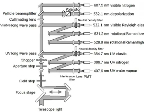
Figure 1.Diagram of CRL’s receiver system. The visible long-wave pass filter picks off approximately 97 % of the received 532 nm light and directs it toward the visible Rayleigh elastic (polarization-independent) channel and transmits the remainder toward the de-polarization and visible nitrogen channels downstream. The pelli-cle beam splitter reflects 50 % of this residual 532 nm light toward the Polarotor and into the depolarization channels’ detector (parallel and perpendicular polarization-sensitive channels, measured using the same PMT on alternate laser shots). The depolarization hard-ware, which was added in 2010, consists of the pellicle beam split-ter, the Polarotor, and the interference filsplit-ter, focusing lens, and PMT to the right of the Polarotor in this figure (McCullough et al., 2017). No other receiver optics were modified in order to reduce the impact of this depolarization upgrade on the pre-existing lidar channels. A consequence of this choice is that the count rates are much higher in the visible Rayleigh elastic polarization-insensitive channel than they are in either the parallel or the perpendicular channel. This fig-ure is based on Fig. 2 of Nott et al. (2012).
In the CRL, optics upstream of the depolarization channel act as a partial polarizer. The optics strongly attenuate the portion of the backscattered lidar intensity which is accepted by the perpendicular channel (which is half of any backscat-tered intensity which has become unpolarized), while attenu-ating by only a small amount the intensity which is accepted into the parallel channel (the other half of the backscattered light which has become unpolarized, plus all backscattered intensity which remains polarized parallel to the transmission plane). The maximum signal in the parallel channel would usually be twice as large as the maximum signal in the per-pendicular channel, even without the partially polarizing ef-fects of the CRL’s receiver optics. The CRL’s optics exacer-bate this effect to a factor of approximately 21 times (Mc-Cullough et al., 2017). This signal mismatch on the PMT, as well as very low signal rates in the perpendicular measure-ments, is detrimental to traditional calculations of d. Tra-ditional depolarization parameter calculations are simple to calibrate but require long integration times and/or integra-tion over large range scales (relative to the time and altitude
scale of variation within the clouds) to produce acceptable uncertainties in the calculated values. The end result is an in-termittent, relatively low-resolution determination ofd. The depolarization parameter determined in the traditional man-ner using the parallel and perpendicular measurements will, in this paper, be calledd1.
The inclusion of an additional CRL measurement channel in the calculations proves helpful and opens the possibility of a new calculation technique for determiningd. Since 2007, CRL has included a polarization-independent Rayleigh elas-tic measurement channel at the same wavelength as the new depolarization channel. This polarization-independent chan-nel has very high signal rates and a high signal-to-noise ra-tio (SNR). It was posited that since all light backscattered to the lidar can be decomposed into parallel and perpendicular components, a linear combination of the signals in the paral-lel and perpendicular channels should be related to the signal measured in the polarization-independent Rayleigh elastic channel, which accepts light of all polarizations. This would allow a measurement ofd which is not as dependent on the low-SNR polarization-dependent measurements. The main advantages of the methods presented here are as follows:
1. We can determine d excluding the low-SNR polarization-dependent channel altogether.
2. We have the flexibility to include simultaneous informa-tion from the low-SNR polarizainforma-tion-dependent channel (the perpendicular channel for CRL) at low resolution to calibrate and improve the high time–altitude resolu-tiondfrom the high-SNR polarization-dependent chan-nel (the parallel chanchan-nel for CRL) and the high-SNR polarization-independent channel.
At CRL, the calibrations required to use the former (the two-channel method) are not particularly practical during routine operations, while use of the latter (the three-channel method) is practical and brings benefits of higher temporal and/or spatial resolution to our measurements of depolariza-tion.
We are not the first to propose a three-channel depolar-ization technique, but these other methodologies could not be implemented on the CRL measurements. Principally, this is because there is differential overlap between the CRL channels. Reichardt et al. (2003), henceforth R2003, use the same three channels we propose here, but in characteriz-ing the optical effects in each channel they account only for differences in efficiency. They assume that all optical el-ements leading to each polarization analyzer have at most the action of a partial polarizer and assume that there is no differential overlap between any measurement channels. Their efficiency ratiosV1,2,3 (required to be “known”
num-ber of specific polarization lidar systems, some of which use a dependent channel with a polarization-independent channel, but none of which sufficiently describe the CRL system. Similar to the R2003 method, the methods in F2016 do not allow for the significant differential overlap contribution in the case of the CRL.
In both the R2003 and the F2016 methods, all measure-ment channels are used simultaneously at identical time and altitude resolutions, and no discussion is made of the impact of having one channel with much lower SNR than the others. The method shown in this paper allows for more flexibility in this regard, and it can be adapted to many types of lidar systems.
Here, we present an extension to the Mueller matrix alge-bra demonstrated in McCullough et al. (2017) for the parallel and perpendicular channels to the polarization-independent channel. We then show that it is possible to determine the depolarization parameter d using only the parallel and polarization-independent channels, plus two calibration fac-tors which must be measured. This scheme, which avoids use of the low-SNR perpendicular signals, yields a depolariza-tion parameter with much higher spatial and temporal res-olution than that produced by the traditional method. The disadvantage is that multiple calibration factors are required, at least one of which varies in altitude and time. When cal-culated using the new method, the depolarization parameter will be referred to asd2.
Sky depolarization is dependent neither on the lidar nor on the way in which the lidar is calibrated, and thusd1≡d2.
We can therefore use the intermittent low-resolution tradi-tional depolarization parameter measurements (d1) to
deter-mine the calibration factors required for the calculation of the depolarization parameter at high spatial and temporal resolu-tion (d2), including tracking the changes in space and time
of the calibration factors. This scheme proves to be the most advantageous method for determining the depolarization pa-rameter using the CRL lidar or, in general, any lidar in which one of the polarized measurement channels has very low sig-nal rates.
Examples of the calibration and calculation procedure for d2, as informed by d1, are provided for 10 March 2013,
which highlight the advantage of the new method. A second example from 14 March 2013 shows some of the nuances in choosing a selection region for the d1 values which are
used in these calibrations based on atmospheric conditions. A more detailed examination of specific case studies using this method is available in McCullough’s PhD thesis (2015). The paper concludes with a discussion and suggestions for future work. The three-channel combined method advocated here is a powerful procedure which allows vastly improved depolarization parameter measurements at CRL, with lower uncertainty and higher spatial–temporal resolution, all with zero extra cost for equipment upgrades or negative impact on the other measurement channels in the lidar. The develop-ment shown here is easily adaptable to any similar lidar and
to any lidar with a single unpolarized and single polarized channel.
An alternative representation of the depolarization is the depolarization ratioδ=d/(2−d). The development in this paper is in terms ofd, but values ofδwill be supplied where relevant.
2 Traditional depolarization method: using parallel and perpendicular measurements to calculated1 Traditionally, the depolarization parameterdis calculated us-ing a combination of parallel- and perpendicular-polarized measurements, as in Eq. (1) (e.g. Gimmestad, 2008, and as used in McCullough et al., 2017):
d1=
2kS⊥ Sk+kS⊥
= 2kS⊥
Sk
1+kS⊥
Sk
= 2
1
k Sk
S⊥+1
, (1)
in whichS⊥is the corrected signal measured by the perpen-dicular channel,Sk is the corrected signal measured by the parallel channel, andkis the depolarization calibration con-stant, which is the ratio of the gains of the parallel and per-pendicular channels. All signalsS have undergone the pro-cesses of correction for pulse pile-up (photon counting de-tection), correction for voltage scaling (analogue dede-tection), merging of photon counting and analogue measurements into a combined profile, co-adding of profiles in time and altitude, and background subtraction. An example of such signals is shown in Fig. 2. In this work, the depolarization parameter calculated using this parallel-perpendicular method will be indicated asd1. Figure 3 provides some examples of d1 as
measured by CRL. 2.1 Calibration ofd1
Lamp and laser calibrations described in McCullough et al. (2017) introduce unpolarized light (simulating d=1 from the sky) to the receiver. Solving Eq. (1) fork, withd1set to
unity, gives k= Sk
S⊥
. (2)
Measurements show thatk=21.0±0.2 for CRL. This value does not change from day to day. Indeed it has been shown to be stable at CRL for several years. It depends only on the partial polarizing effects of the receiver’s optical components and, in lidars which have separate PMTs for the parallel and perpendicular measurement channels, PMT gain.
2.2 Advantages and disadvantages to the traditionald1 method
Calculations ofd1are straightforward, requiring a single
Figure 2. Corrected photocounts from 10 March 2013.(a, c, e)gives the corrected photocounts for the perpendicular(a), parallel(c), and polarization-independent Rayleigh elastic(e)channels. The corresponding absolute uncertainties, in units of photocounts, are plotted in(b, d, f). All data points with a signal-to-noise ratio less than 1 have been removed and are coloured white. Because of the combined photon counting and analogue measurements at CRL, these uncertainties are not simply the standard deviation of the photocounts reported in the left column of plots. Resolution is 20 min×7.5 m.
this method, specifically for CRL lidar, and for any lidar for which the maximum parallel signal strength far exceeds the maximum perpendicular signal strength.
For CRL, low count rates in the perpendicular channel mean that much averaging in time and/or space is required to calculated1to within an acceptable uncertainty. The user
may decide which information (vertical spatial vs. tempo-ral) is most important for addressing their scientific ques-tions. Figure 2 gives an example of co-added count rates in each channel at a resolution of 20 min×7.5 m. At best, CRL can produce only values of d1 with either low time
resolution or low altitude resolution. Cloud properties can change on the vertical scale of metres (e.g. for liquid lay-ers within ice clouds) and minutes (depending on the speed of the clouds carried over the lidar’s location), so the utility of cloud depolarization measurements is linked to the reso-lution at which they can be acquired. The general require-ment for high spatial and temporal resolution in determining cloud microphysical parameters such as liquid water con-tent is stated by numerous authors. Requirements for sub-100 m sampling are given by Mioche et al. (2017), Loewe et al. (2017), and Hogan et al. (2003), with requirements on the scale of 50 m given even earlier by Ramaswamy and
Detwiler (1986) and Korolev et al. (2007) and recently by Sotiropoulou et al. (2014) and Solomon et al. (2015). Aver-aging the depolarization parameter measurements over too large an area of time and space smears localized values of low and high depolarization to an appearance of a smooth re-gion with an intermediate value. Incorrect interpretations of such over-averaged measurements are inevitable, as shown by the analysis of CALIOP satellite lidar measurements in Cesana et al. (2016).
Even with substantial co-adding of bins, there are fre-quently regions of the time–altitude measurement space (par-ticularly at higher altitudes, where atmospheric density is lower) for which the CRL perpendicular measurement chan-nel has too few counts to make a calculation. There are com-monly measurement bins for which zero photons are mea-sured, leading to intermittent calculatedd1values.
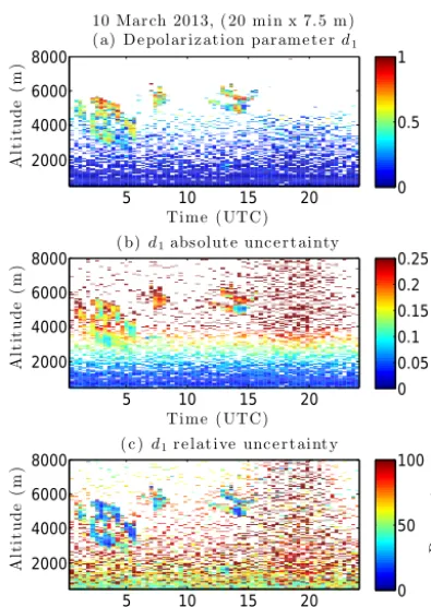
Figure 3. (a)Traditional methodd1depolarization values from 10
March 2013.(b)Absolute uncertainties associated with thed1 val-ues, in units of depolarization parameter.(c)Relative uncertainties, in units of percent. Any locations with photocount signal-to-noise ratios less than 1 have been removed and are coloured white. No points have been removed based on calculated uncertainty ind1.
Rayleigh elastic channels. In this work, the depolarization parameter calculated using the parallel and polarization-independent signals will be indicated asd2. For CRL, count
rates in each of these channels are much higher than the max-imum count rates in the perpendicular channel, by a factor of 10 to 50 for parallel and by a factor of 200 for polarization-independent. Less co-adding leads to higher-resolution cal-culations of the depolarization parameterd2.
McCullough et al. (2017) developed a full Mueller ma-trix calculation for the signals in each depolarization chan-nel. Under conditions which are true for the CRL lidar, these signal equations are expressed as Eqs. (3) and (4):
Sk= (3)
GPMTkbOk⊥(z)Ilaser
2 (M00+M10+(M01+M11)(1−d)),
S⊥= (4)
GPMT⊥bOk⊥(z)Ilaser
2 (M00−M10+(M01−M11)(1−d)), in whichSkandS⊥are the signal rates measured in the par-allel and perpendicular channels, respectively; GPMTk and GPMT⊥are the combined gains (or attenuations) of the fo-cusing lens, interference filter, and photomultiplier tubes for
each channel (where GPMTk=GPMT⊥ for CRL as they share the same PMT and associated optics);bis an arbitrary gain factor used to normalize the atmospheric scattering ma-trix;Ok⊥(z) is the overlap function, containing all height-dependent variations in lidar signal and named for the largest of these contributions which is the geometric overlap func-tion;Ilaseris the laser intensity;Mxx are individual elements of the 4×4 Mueller matrixMwhich describes the combined optical effect of all optics in the shared beam path for the par-allel and perpendicular channel which are upstream of the Polarotor; anddis the depolarization parameter of the atmo-sphere. The values Sk,S⊥, and d are all understood to be functions of altitude,z, and time,t.
A similar argument to that of McCullough et al. (2017) may be made to develop an expression for the signal in the polarization-independent Rayleigh elastic channel. The ma-trix expression for the received Stokes vector,IR, for the
polarization-independent channel is given in Eqs. (5) and (6), corresponding to McCullough et al. (2017, Eq. 8). This chan-nel does not contain a polarizer. Some optics such as the telescope and focus stage are in common for all channels, but others are different, for example the visible long-wave pass filter: the polarization-independent Rayleigh channel receives a reflection off this optic while the parallel and perpendicular channels receive the transmission through it. Thus, the matrix for optics upstream of the polarization-independent PMT is given byTrather thanMused for the polarized channels;GPMTR is used for the combined gains
(or attenuations) of the focusing lens, interference filter, and photomultiplier tube associated with the polarization-independent channel; andOR(z)is used for the overlap
func-tion. OR(z) differs from Ok⊥(z) because of the different beam paths taken through the receiving optics of the instru-ment to reach each PMT and the possibility that each channel focuses differently onto its PMT.
IR=GPMTR
T00 T01 T02 T03 T10 T11 T12 T13 T20 T21 T22 T23 T30 T31 T32 T33
(5)
bOR(z)
1 0 0 0
0 1−d 0 0
0 0 d−1 0
0 0 0 2d−1
Ilaser
1 1 0 0
IR=GPMTRbOR(z)Ilaser
T00+T01(1−d) T10+T11(1−d) T20+T21(1−d) T30+T31(1−d)
The signal rateSRin Eq. (7) is the intensity element of the
Stokes vectorIR:
SR=GPMTRbOR(z)Ilaser(T00+T01(1−d)). (7)
The goal is to determine an expression for the depolariza-tion parameter using only the signals from the parallel and polarization-independent Rayleigh elastic channels, Sk and SR. First, the polarization-independent channel’s signal
equa-tion (Eq. 7) is solved forbIlaser (a quantity which cannot be
truly known during any given measurement and thus we de-sire to eliminate it):
bIlaser=
SR GPMTROR(z)
1 T00+T01(1−d)
. (8)
Substituting Eq. (8) into the parallel channel’s signal equa-tion (Eq. 3) and solving for the depolarizaequa-tion parameter (now labelledd2) gives
Sk=
GPMTkOk⊥(z) 2
SR GPMTROR(z)
(9)
M00+M10+(M01+M11)(1−d2) T00+T01(1−d2)
,
d2=1+ 1 2
GPMTkOk⊥(z)
GPMTROR(z)
SR
Sk(M00+M10)−T00 1
2
GPMTkOk⊥(z)
GPMTROR(z)
SR
Sk(M01+M11)−T01
, (10)
d2=1+ 1 2
SR
Sk(1+
M10
M00)−
G
PMTROR(z)
GPMTkOk⊥(z)
T00 M00 1 2 SR
Sk(
M01
M00
+M11
M00)
−GPMTROR(z)
GPMTkOR(z)
T01
M00
, (11)
in which Sk and SR are measurements, while Mxx, Txx, GPMTk, andGPMTRmust be determined by calibration
mea-surements. Overlap functions are in general difficult to de-termine for lidars. They tend to change with laboratory tem-perature (which we cannot control precisely), alignment of transmitter mirrors (adjusted at CRL approximately 2 to 3 times per year), and alignment of the laser beam to the sky (adjusted nightly at CRL). Here, the “overlap function”O(z) includes both geometric overlap (varies in altitude and time) as well as any other factors which vary in altitude (though they may be constant in time). The overlap function will be eliminated where possible, and available means will be used to determine it via calibration otherwise.
Five calibration factors are thus needed: M01
M00,
M10
M00,
M11
M00,
GPMTROR(z)
GPMTk⊥Ok⊥(z)
T00
M00, and
GPMTROR(z)
GPMTk⊥Ok⊥(z)
T01
M00. Some information
is already known. Polarized and unpolarized white light char-acterization tests in McCullough et al. (2017) found that
M01
M00=0.91±0.002 for CRL. Thus, each channel has a
dif-ferent gain, indicated by M016=M00. These tests also
en-sured that the parallel channel is well-aligned with the po-larization plane of the outgoing laser beam, and they demon-strated that M11=M00 and M01=M10, indicating an
ab-sence of cross-talk between the parallel and perpendicu-lar channels; no parallel-poperpendicu-larized light gets into the per-pendicular profiles, and vice versa. An extension to one of these detailed characterization tests was carried out for the polarization-independent channel. Polarized light intro-duced to the receiver at a variety of angles show that if there is any sensitivity to polarization in the “polarization-independent” Rayleigh elastic channel, this effect is orders of magnitude smaller than the uncertainty in routine lidar mea-surements and does not affect analyses (Appendix A). As the CRL polarization-independent Rayleigh elastic channel has been shown to be insensitive to changes in polarization (i.e. responds independently of polarization of incoming light), T01=0. Were this not the case, its signal would depend on
the depolarization effects of the atmosphere. Therefore, the equation ford2simplifies to
d2=2−
2 1+M10
M00
!
GPMTROR(z) GPMTkOk⊥(z)
T00 M00 Sk SR . (12)
None of the parametersM00,M10, andT00 are needed
in-dividually. Nor is any individual overlap functionO(z) re-quired, although a ratio of these is included. The ratio of overlap functions is unlikely to be stable in time, and this must be taken into account when calibrating. We require only two calibration factors: M10
M00, which is stable in time and has
already been determined, and GPMTROR(z)
GPMTk⊥Ok⊥(z)
T00
M00, which can
vary and will likely require more frequent calibrations. For clarity, we define a new variableY (z)= GPMTROR(z)
GPMTk⊥Ok⊥(z)
T00
M00,
such that
d2=2−
2 1+M10
M00 ! Y (z) S k SR . (13)
3.1 Calibration ofd2
The calibration profilesY (z)must be determined befored2
can be calculated. Unlike all other calibration terms in the equation for depolarization parameter using the d2 setup, Y (z)may vary with altitude. It contains the overlap functions Ok⊥(z)andOR(z)in a ratio indicating the differential
over-lap between the polarization-independent and the depolariza-tion photomultiplier tube viewing geometries. Equadepolariza-tion (13) is solved for the calibration profile:
Y (z)=1 2
1+M10 M00
SR Sk
(2−d2). (14)
In order to set d2=1 in Eq. (14), enabling us to solve
will not suffice for this calibration because of the altitude de-pendence of the calibration profile we seek. The calibration calculation with the depolarized-lidar setup becomes Y (z)=1
2
1+M10 M00
SR Sk
. (15)
Since it is possible to change gain settings on the paral-lel PMT from time to time, it may be desirable to keep M01
M00
as a term in d2 calibrations. In that case, an identical
un-polarized white light calibration may be done while solving Eq. (13) for the entire term 2Y (z)
1+M10 M00
!
. This large calibration term could then be applied to measurements taken the same day as the calibration. This possibility is not explored fur-ther here, as M01
M00 =0.91±0.002 was not changing for CRL
during the measurement period in question. 3.2 Advantages and disadvantages ofd2
There are more practical considerations for thed2calibration
than there are for thed1calibration. The glassine sheet
atten-uates all signals, and it is important to have calibration mea-surements from all relevant lidar heights (for CRL preferably up to 10 to 20 km altitude). Thus, particular atmospheric sit-uations are helpful during the calibration, especially those with highly backscattering clouds at middle and high alti-tudes. It takes several hours to do this measurement to build up a good calibration profile.
A critical disadvantage is that the “constant” profileY (z) contains overlap functions which could change with time, such as each time the laser beam is realigned to the sky, and when there is a change in laboratory temperature. There-foreY (z)must be determinedeach night(unless experience shows that a less frequent calibration suffices) by putting a depolarizing sheet over the lidar, accumulating sufficient counts (which are attenuated during the calibration) to de-termine the calibration profile, then removing the sheet and making actual measurements of the atmosphere for the re-mainder of the night. Realistically, CRL can be calibrated in this way or it can measure the atmosphere, but not both in any given night. If the calibration profiles are determined to be sufficiently constantfrom night to night, this calibra-tion method could be used every couple of days in between days of good measurements. (In this case, an uncertainty will be introduced to d2, which can be estimated by examining
the typical variation in profiles ofY (z)and propagating this value through the equations ford2. Each lidar retrieval’s
tol-erance for additional uncertainty in its d2 calculations will
determine the level of variation which can be tolerated in Y (z).)
While possible for a lidar with a local operator, this proce-dure is not practical for a remotely operated instrument such as CRL. Nonetheless,d2offers attractive advantages due to
the higher signal rates involved: the resolution of d2far
ex-ceeds that of d1 for CRL, and measurements are available
to higher altitudes. It is possible circumventd2’s calibration
disadvantages by informing the calculation usingd1values
from the same measurement period. This procedure is dis-cussed in the following section, recalling that bothd1andd2
represent the true depolarization state of the atmosphere,d.
4 Combining methods: using low-resolutiond1to initialize high-resolutiond2
Calibration constants required for calculations ofd1and of d2 may all be determined through special calibration
mea-surements with the lidar (McCullough et al., 2017, ford1;
Sect. 3.1 ford2). This provides two nearly independent
re-sults for the depolarization parameter for a particular mea-surement period:d1with a well-understood calibration
con-stant, but with low-resolution values, andd2with more
com-plicated calibration constants which can change over time, but with higher-resolution values and more coverage in space and time.
A more advantageous approach is to combine these two methods, using the low-resolutiond1 values to inform the
high-resolutiond2values for that same day’s measurement.
In effect, high-resolution d2 values can be calibrated daily
using low-resolutiond1values rather than using a separate
special calibration procedure.
4.1 Calibration method usingd1to determineY (z)and apply it to measurements ofd2
It is possible to solve initially for the depolarization param-eter d1 at high altitude resolution but low time resolution,
feed it into the calibration Eq. (14), and solve for a nightly calibration profile. Then this profile can be used in the ex-pression for d2 (Eq. 13), even at resolutions not possible
with the original d1 measurements. Calibrations to
deter-mine theY (z)profile may be carried out during any reason-able period which contains simultaneous measurements from all three channels: parallel, perpendicular, and polarization-independent. The methodology is as follows:
1. Parallel and perpendicular measurements are used to de-termine the depolarization parameterd1using the
tradi-tional method at high altitude resolution but low time resolution. Many data points may still be missing be-cause perpendicular count rates are low.
2. Eq. (14) is used to calculateY (z)at the same high alti-tude resolution, but low time resolution, as the calcula-tions made ford1. In contrast to the method in Sect. 3.1,
this time no special hardware is put in place, and there-fored2is not set to unity in the equation (i.e. we cannot
themselves are fed into Eq. (14) as the values ford2in
order to determine theY (z)values at each time and al-titude.
3. TheseY (z)values are combined to create a single cal-ibration profile of Y (z)for the measurement period at high altitude resolution.
4. Parallel and polarization-independent measurements are then co-added to their optimal time and altitude resolu-tions. Their higher photocount rates mean that less co-adding is required to achieve the same SNR that is pos-sible with the perpendicular measurements at low reso-lution.
5. Finally, the single Y (z) profile for the night is ap-plied to each profile of the high-resolution parallel and polarization-independent signals to calculated2. The
re-sult is that thed2values calculated in this way can have
higher resolution, and retain more data points, thand1.
The method described here is most advantageous for CRL’s depolarization calculations, as demonstrated in the following sections.
5 Measurements to demonstrate the three-channel method
A night of regular operation measurements (i.e. not a spe-cial calibration run) on 10 March 2013, with measure-ments made in all three channels (parallel, perpendicular, and polarization-independent), is used for this demonstration. 5.1 Signals and uncertainties in each channel
The night of 10 March 2013 was clear below 3500 m with several clouds above this height. The clouds are not particu-larly thick; signal is visible above each of them in the parallel and polarization-independent Rayleigh elastic channels. The entire night’s measurements and associated uncertainties are shown in Fig. 2. The plots here have been photon-counting dead-time corrected, analogue range scaled, and dark count corrected, as well as co-added and background subtracted. Co-adding resolution was chosen to be 20 time bins (20 min) and 1 altitude bin (7.5 m) in order to have sufficient perpen-dicular signal for analyses while retaining as much vertical resolution as possible. Photocount rates in the perpendicu-lar channel are exceeded by those in the parallel channel by a factor of between 10 and 50 times, and by those in the polarization-independent Rayleigh elastic channel by a factor of approximately 200. Consequently, the SNRs in the latter two channels are far superior to that in the perpendic-ular channel. The absolute uncertainties include the statisti-cal measurement uncertainties carried through the described processing using standard error propagation methods. Be-cause of the combined photon counting and analogue mea-surements at CRL, these uncertainties are not the simply the
standard deviation of the photocounts reported in the top row of plots, although this element is the dominant contributor to the overall uncertainty values. The statistical uncertainty of the merged profiles has been discussed in McCullough (2015).
5.2 Depolarization parameterd1as determined by the traditional method
The depolarization parameterd1is determined using the
par-allel and perpendicular measurements following Eq. (1), re-sulting in the upper panel of Fig. 3. The associated absolute uncertainty is calculated using standard error propagation equations and is shown in the centre panel of Fig. 3. For ex-ample, the measurements at 03:30:00 UTC at 3000 m altitude have a depolarization ratio of approximatelyd1=0.6±0.1
as read from the upper and centre panels. To calculate the relative uncertainty shown in the lower panel of Fig. 3, the absolute uncertainty was divided by the associated value of d1and expressed as a percent; thus, the same measurement
as read from the upper and lower panels is approximately d1=0.6±17 %. Both expressions for uncertainty are
use-ful in interpreting the depolarization values. This measured depolarization parameter value ofd1=0.6 corresponds
ap-proximately to a depolarization ratio value ofδ=0.43. The high depolarization parameter values at 04:00:00 UTC, at 5500 m altitude, indicate that the cloud is composed of par-ticles which are not homogeneous spheres; in context, this means that the cloud is likely composed of ice particles. The uncertainty ind1in this region of the cloud is
approx-imately 12 %. For the small cloud at 07:30:00 UTC, there is less certainty. There, the d1 values indicate a mix of high
and low depolarization varying between 0.4 and 0.8 in a rather noisy fashion. The uncertainty in this small cloud is ±0.25 or higher, indicating more than 30 % relative uncer-tainty. The edges of all clouds have high uncertainty as well. While a general interpretation of icy clouds in a clear atmo-sphere is possible, depolarization parameter measurements with higher resolution and/or smaller uncertainty would be better. If there are clouds above 6000 m altitude, d1 is not
sensitive to them because of the low count rates in the pendicular channel. The extremely low signal rates in the per-pendicular channel lead to many time–altitude points with in-sufficient SNR (<1) to be considered. Consequently, much of the time–altitude space in the plot ofd1is blank.
5.3 Determining the calibration profileY (z)
Next, the polarization-independent channel is brought into the evaluation, and the calibration profileY (z)is determined. 5.3.1 Calculations ofY (z)for each data point
Using Eq. (14), a value ofY (z)is determined for each data point in time and altitude, based on thed1values shown in
Figure 4. (a)TheY (z)calibration values from 10 March 2013 indi-vidually for each data point.(b, c)Absolute and relative uncertain-ties, respectively, in the calculated individual values ofY (z).
The uncertainties are calculated assuming uncorrelated er-rors, using standard error propagation methods.
If there were a good signal in the perpendicular channel, and thus good calibration measurements for each altitude, it would be possible to calibrate the lidar measurements profile by profile. However, there are frequently too few perpendic-ular measurements to make good statistics in this manner. It is feasible to determine one single profile for the night (per-haps even persisting longer) to use as a function ofY (z)with altitude. The differential overlap function may be changing with such factors as temperature of the lab and laser align-ment. Differential overlap is commonly known to vary little within one night, varying more between nights, particularly when the lidar has been cooled down and warmed back up in the interim or when the lidar has been realigned to the sky. The latter procedure is carried out at the beginning of each very clear night. Conversely, the GPMTR
GPMTk⊥ and
T00
M00 portions
of Y (z) should be relatively stable provided no instrument parameters are changed. Therefore, the combined calibration factorY (z) is expected to vary slowly with time following the temporal trends of the differential overlap function.
Figure 5. (a)TheY (z)calibration values from 10 March 2013 with the various fits to the night’s measurements.(b)Magnified portion of the plot on the left to show differences between the lines.
5.3.2 Combining individual measurements into a single
Y (z)for the night
First, a mean profile in altitude is taken based on the calcu-lated individual values. The propagated uncertainty reduces drastically as a large number of profiles are combined (just as for any co-adding procedure). A smooth profile was desired so that the profile would not be unduly influenced by small clouds, for example. A 10-point moving-average filter was applied to the mean profile to smooth it in altitude.
A number of options were tested to determine the opti-mal profile ofY (z)with altitude, and acceptable results were found using a power law fit to the entire profile, as shown in Fig. 5. A power law of the formy=axb+cwas found to fit the calibration data (y, the smoothed mean profile) with altitude (x) with goodness-of-fitR2of greater than 0.998 in every case studied. For the example data shown in this sec-tion, the coefficients to the power law are given bya,b, and c, with 95 % confidence bounds in parentheses:
a=1.152×10⁵(1.082×105,1.223×105) b= −1.026(−1.036,−1.017)
c=31.81(31.29,32.34).
Figure 6. (a)The residuals of individualY (z)profiles for 10 March 2013 are shown after subtracting the nightly power law fit. Solid black lines indicate±1σof the measured profiles. The dashed line at zero emphasizes the lack of bias in the fit.(b)The number of valid data points forY (z)at each altitude. More data points are available anywhere photon signals are high, such as at low altitudes and inside clouds. The deviation of the residuals from zero in the left figure above 6000 m is explained by the lack of data points above this altitude.
In Fig. 5, four curves are plotted over the individual pro-files: the mean profile, the upper and lower bounds on the mean profile based on the mean profile’s uncertainty, the power law fit function, and the upper and lower bounds on the power law fit function based on the RMSE in the fit it-self. Note that the RMSE in the fit dominates the error in the mean profile. It was determined that the measurement error in the mean profile could be neglected in the fitting process for this reason. This quantity is quite stable over the course of the night, indicated by the near coincidence of all profiles plotted in each panel of Fig. 5 and the lack of a trend in time at any altitude in Fig. 4.
The residuals for the power law fit for 10 March 2013 are given in Fig. 6. For the altitudes used in CRL analysis there is no trend in the residuals, and therefore the power law fit is acceptable. In the left panel, the residuals are given as the difference between the individualY (z) profiles and the nightly power law fit. Each of these residual profiles can also be expressed as a percent residual profile (not shown). Be-low 3500 m altitude, the residuals are always smaller than the mean percent uncertainty in the individualY (z)profiles themselves, and the values are comparable up to 4500 m. This indicates that the power law fit is at least as good be-low these altitudes as any of the individual profile measure-ments themselves. The large amounts of scatter and bias above 6000 m can be explained by the paucity of valid data points at those altitudes. The right panel of Fig. 6 indicates fewer than five valid points going into theY (z)calculations at each of those altitudes. This is the region above the top-most clouds visible in Fig. 4. Everywhere below 6000 m, the residuals are smaller than 20 % of the value of the nightly power lawY (z)profile.
5.3.3 Variation in the profileY (z)with changing co-adding resolution and with different dates To check whether the profile ofY (z)with altitude is different depending on the co-adding of the original data, the calibra-tion procedure was carried out for the following resolucalibra-tions of 10 March 2013 data: (10 min×7.5 m), (20 min×7.5 m), and (10 min×37.5 m). To check whether the profile changes with time on scales longer than 1 day, data from 11 March 2013 and 14 March 2013 were also examined, mostly at 20 min×7.5 m resolution. The general form of these fits is unchanging for these days in March 2013, as shown in Fig. 7. This suggests that it is appropriate to use the calibration pro-file from one day to make d2 measurements for a nearby
day. This could be useful should the perpendicular channel be temporarily unavailable. Also, there are certain sky con-ditions which are not well-suited for the determination of the calibration profile. Section 6 contains an example of a mea-surement day containing just such a situation. In that case, a nearby day’s calibration may be preferable to its own day’s calibration.
5.4 Determinations ofd2at low resolution
A sample from 10 March 2013 is given in Fig. 8, withd2
cal-culated using Eq. (13) and the calibration profiles discussed in Sect. 5.3.2. The resolution is kept at 20 min×7.5 m, the same as it is for the calculation ofd1.
The values retrieved for d2 as informed by d1 give
re-sults 06d261 as required. Regions of high depolarization
parameter are visible within the clouds, as they are for the traditional d1 results in previous plots. These regions also
have low absolute uncertainty, as do the very low altitudes where the density of the atmosphere is large. These plots of d2also show much better coverage of the space and time
Figure 7. (a) Plots of second-order power law fits to the calculated profiles ofY (z)for the test dates and resolutions listed in Table 1.
(b)Residuals of each profile from the mean power law fit profile. Compare this panel to Fig. 6a. The residuals are of similar magnitude to the uncertainties in the individually measuredY (z)profiles.
Figure 8. (a)Thed2depolarization values from 10 March 2013,
calculated at the same resolution (20 min×7.5 m) as the d1
val-ues shown in Fig. 3. Higher-resolutiond2results follow in Fig. 11. (b)The uncertainties associated with thed2values are all in units of
depolarization parameter.(c)The relative uncertainties are in units of percent. The current figure demonstrates two advantages of the
d2method over thed1method when the resolution is kept constant:
better coverage of time and space and lower uncertainty for each data point.
SNR. There is now meaningful depolarization parameter in-formation in all regions of the plot.
While data ford1end entirely at around 2000 m altitude,
except in the cloud, data ford2extend to above 5000 m with
uncertainty smaller than±0.25, and less certain values are calculable at yet higher altitudes. The cloud features are bet-ter delineated withd2data and have lower uncertainty than
those calculated asd1.
Some regions do haved2 relative uncertainty
approach-ing 100 %, but these are regions with depolarization parame-ter values<0.1 (which corresponds to a depolarization ratio value ofδ <0.05). A measurement ofd=0.1±0.1 is still a meaningful value indicating non-ice particles or clear air. The values ofd1in the clouds at 04:00:00 UTC, 5000 m, have, in
some locations, values ofd=0.6±0.25. This is a less defini-tive measurement in terms of interpretation since the low end of the uncertainty range would indicate liquid particles while the high end of the uncertainty range would indicate ice. In contrast, the same cloud regions in thed2 plot have values
ofd=0.6±0.07 and a relative uncertainty less than 10 %, which is a clear indication of ice.
The one location thatd1appears better constrained thand2
is the horizontal strip along 1000 m altitude. Examining the uncertainty plots,d1has less than 0.04 absolute uncertainty
in this location, whiled2’s is closer to 0.06. The reason for
this is the use of the analogue counting channel in the paral-lel and polarization-independent counts which go into creat-ingd2. As the processing routine switches over from photon
Table 1.Fitting coefficients (a,b, andc; fitting a second-order power law of the formy=axb+c) and goodness of fit (R2and root mean square error (RMSE)) for various dates, time resolutions (time res.), and altitude resolutions (alt. res.) in March 2013 used for determining calibration functionY (z). Days marked with∗used only a portion of the data available for that day: clear sky or thin clouds only.
Test Date Time res. (min) Alt. res. (m) a(bounds) b(bounds) c(bounds) R2 RMSE
i 10 March 20 7.5 115 200 (108 200,122 300) −1.026 (−1.036,−1.017) 31.81 (31.29,32.34) 0.998 1.523 ii 10 March 10 35.5 48 260 (29 866,67 870) −0.8896 (−0.9555,−0.8238) 27.36 (22.72,32) 0.982 4.750 iii 10 March∗ 10 7.5 92 540 (86 810,98,280) −0.9876 (−0.9975,−0.9777) 26.04 (25.54,26.62) 0.998 1.594 iv 11 March∗ 20 7.5 164 900 (154 200,175 500) −1.085 (−1.095,−1.075) 35.04 (34.55,35.53) 0.998 1.542 v 11 March 2 15.0 310 200 (230 500,390 000) −1.172 (−1.213,−1.131) 26.44 (24.62,28.26) 0.985 4.753 vi 14 March∗ 20 7.5 567 700 (514 400,621 000) −1.304 (−1.318,−1.289) 35.71 (35.29,36.12) 0.996 1.860 vii 14 March∗ 20 7.5 407 900 (383 400,432 400) −1.217 (−1.227,−1.208) 38.6 (38.21,38.98) 0.998 1.504
5.5 Comparing the two methods:d2reproducesd1 To ensure that the results for d calculated using the new method (d2; Fig. 8) are valid, they must be compared with
those calculated using the traditional method (d1; Fig. 3) and
have the same values to within the uncertainty of both of the measurements.
To make the comparison, each plot had the following steps applied in sequence:
1. smoothing by 3×3 moving average filter, for a smoothed resolution of 60 min×22.5 m;
2. removal of any data points which are surrounded on three or four sides by an empty data point, done recur-sively twice such that isolated groups of two data points will also be eliminated;
3. removal of any data points which do not exist in both of the plots.
A scatter plot can then be created of all (d1,d2) pairs. For
clarity, this information is represented by plotting the natural logarithm of the number of data points present at each (d1, d2) location, binned in a 0.02×0.02 grid. In this way, we
see the overall trend of the measurements. This is shown in Fig. 9. Red points indicate that more than 60 (d1,d2) pairs
lie at that location, while blue points indicate the locations of fewer than 2 (d1,d2) pairs. The black line in this figure is a
1 : 1 line for reference. It is not a regression line, but it does demonstrate the 1 : 1 trend betweend1andd2values.
In most altitude and time bins, there is no difference be-tween the depolarization parameters calculated to within the limits of their combined uncertainties. Of all data points in the original d1 and d2 plots for this time–altitude region
(Figs. 3 and 8), none contain only ad1measurement, 65 %
contain only ad2measurement, and 35 % contain both ad1
and ad2measurement. All data points for which there is both
ad1and ad2measurement are included in Fig. 9. Of these,
the measurements are significantly different from each other in 0.1 % of cases. For the remainder of the measurements in Fig. 9 (99.9 % of cases),d1=d2to within their uncertainties.
Of these statistically equal cases,d1has the lower uncertainty
for 15 % of the points (almost exclusively from below 3000 m
Figure 9.Scatter plot ofd1vs.d2, binned with a grid of 0.02×0.02.
Colour of point gives ln (number of data points at that particular (d1,
d2) grid location). A 1 : 1 line is also given. This is not a regression,
but demonstrates the basic equivalence of the two methods.
altitude, where count rates in the perpendicular channel are high), whiled2has the lower uncertainty for the other 20 %
of the points (some points below 3000 m, but most are above that altitude). If we omit the smoothing step in the Fig. 9 analysis, the number of significantly differentd1andd2
val-ues increases to only 3 %. This is encouraging, as it shows that the CRL’s parallel and polarization-independent method (d2) is as valid as its parallel and perpendicular method (d1).
These tests indicate thatd1andd2are similar for almost all
the times when they can be measured simultaneously, giving confidence thatd1andd2are the same quantity and thatd2
values with their increased spatial and temporal coverage can be relied on.
In almost all situations, thisd2 procedure provides
mea-surements of d with significantly reduced uncertainty as compared to the d1 procedure which relies on the
perpen-dicular channel. The following sections demonstrate the true power of thed2method: access to depolarization ratio
Figure 10.Thed1depolarization values from 10 March 2013, with
10 min×7.5 m resolution, excluding anywhere with more than 0.2 absolute uncertainty in units of depolarization parameter: (a) d1
values, (b)uncertainties associated with thed1 values in units of
depolarization parameter, and(c)relative uncertainties in units of percent.
5.6 Determinations ofdat higher resolution
Using the traditional method,d1is calculated a higher
reso-lution of 10 min×7.5 m, keeping only data for which pho-ton count SNR >1 and for which absolute d1 uncertainty <0.2. The resulting plots in Fig. 10 readily show a deteri-oration in interpretability as compared to the plot using the lower-resolution 20 min×7.5 m values ofd1(calculated in
Sect. 5.2). There are large differences in data coverage at this higher resolution, and there are atmospheric features which are no longer discernible.
Conversely, a calculation of d2 at the higher resolution
remains meaningful. The example illustrated here uses the low-resolution 20 min×7.5 m values of d1 (calculated in
Sect. 5.2) and the resulting Y (z) calibration profile (calcu-lated in Sect. 5.3.2). These low-resolution calcu(calcu-lated val-ues are then applied to parallel and polarization-independent photocount measurements at twice the time resolution: 10 min×7.5 m. The resulting higher-resolution values ofd2
are given in Fig. 11, retaining in the plot all data for which absolute uncertainty is less than 0.2.
The deficiencies of d1 and advantages to using d2 are
clearly seen. There are large differences in data coverage
Figure 11.Thed2depolarization values from 10 March 2013, with
10 min×7.5 m resolution, excluding anywhere with more than 0.2 absolute uncertainty in depolarization parameter units.(a)d2
val-ues;(b)uncertainties associated with thed2values in units of
de-polarization parameter;(c)relative uncertainties in units of percent. The calibration profile is based on 20 min×7.5 m resolution calcu-lations.
at this higher resolution, and there are features visible ind2
which are not visible ind1:d1can barely discern that there
is a cloud at all at 13:30:00 UTC, whiled2still clearly gives
the cloud’s shape.
6 Importance of calibration selection region
The calibration profileY (z)can only be calculated based on valid values ofd1, which can only be calculated in regions
where the lidar assumptions of single scattering and low ex-tinction are valid. In some meteorological cases, these as-sumptions are not appropriate. The following example illus-trates the importance of selecting an appropriate region in time and altitude for the calibration. A co-adding resolution of 20 min×7.5 m was selected for this comparison. This pro-vides sufficient photons in the perpendicular channel to make calculations.
Figure 12.Polarization-independent Rayleigh elastic photocounts from 14 March 2013. Note the logarithmic colour bar used for this plot. These photocounts have been dead-time corrected, co-added, and background subtracted.
Figure 13. (a)Thed1depolarization values from 14 March 2013, at 20 min×7.5 m resolution.(b)The uncertainties associated with the d1values are all in units of depolarization parameter.(c)The
relative uncertainties are in units of percent. Values indicated for the interior of the optically thick cloud are not valid, although they have been calculated.
the upper regions of the cloud. The cloud descends to the ground by 12:00:00 UTC and remains there for many hours. Values ofd1will not be valid in the thick cloud and are not
calculable at all above it.
The d1 depolarization parameters are presented with
un-certainty and relative unun-certainty in Fig. 13. IndividualY (z) calculations are made next for each time–altitude measure-ment point for the entire time and altitude range for this
14 Mar ch 2013, ( 20 min x 7.5 m) calibr at ion value sY(z)
Time ( UTC)
A
lt
it
u
d
e
(m
)
0 5 10 15
2000 4000 6000 8000
0 50 100 150 200
Box B
Box A:ent ir e plot ar e a
Figure 14.Context plot of all individualY (z)values for 14 March 2013. Box A indicates the region included in the nightly profile which includes all measurements. The profiles from this selection are given in Fig. 15a. Box B indicates the region included in the nightly profile which excludes any regions with thick clouds. This clear-sky region has profiles given in Fig. 15b.
Figure 15.Profiles of fits toY (z)calibration values for 14 March 2013. Panel(a)uses profiles from all measurements from the mea-surement period, which corresponds to those in box A of Fig. 14. Panel(b)uses only profiles which include clear sky, which are those indicated in box B of Fig. 14. All regions with thick clouds have been excluded.
day. These are plotted in Fig. 14. The analysis of determin-ing a representative calibration profile for this day, and us-ing it to calculated2, was performed twice: once including
all the data (Figs. 14, box A, 15a, and 16), and again taking into account only regions without thick clouds (Figs. 14, box B, 15b, and 17). We can see at once that using the whole re-gion (box A) will not be appropriate: the value ofY (z)at par-ticular altitudes, such as at 1000 m, is not constant throughout the time series.
Figure 16 illustrates the perils of blindly choosing a cali-bration region of sky. The “default” region, box A in Fig. 14, which encompasses the entire data region, does a poor job of producingd2 values which mimic those given by d1 in
Fig. 13. Furthermore, the resultingd2values show high
photo-Figure 16. (a)Thed2depolarization values from 14 March 2013,
using all data available for that day to influence the calibration pro-file.(b)The uncertainties associated with thed2values are all in
units of depolarization parameter.(c)The relative uncertainties are in units of percent.
count plot (Fig. 12) reveals that the current example has a bad choice of calibration region.
Consider next the plots of Fig. 17, in which a more care-ful calibration region, box B, was selected. The entire region with the thick cloud has been excluded from the calculation of the calibration profile. Then this conservative profile has been applied to the entire data space to produce thed2plot.
An examination of the difference between thedvalues shows that in almost all cases for the beginning of the measurement, the values ofd1andd2are the same to within±0.1 in
depo-larization parameter units. The only location which does not match well (though differences are no larger than those when using box A) is within the thick cloud, where the originald1
measurements are invalid to start with.
Most of the measurement is good; within the upper re-gions of the thick cloud, it is not. Rere-gions of CRL plots which are least trustworthy in terms of atmospheric inter-pretation are those which lie above strongly scattering lay-ers. Although there is well-understood precision regarding the number of photons returned from these higher regions to the lidar (and therefore the calculated uncertainty is quite low), their interpretation is less clear as multiple scattering cannot be ruled out. Thed2calibration procedure is not
han-dled autonomously at this time, as the calibration region must
Figure 17. (a)Thed2depolarization values from 14 March 2013,
using only clear-sky and regular cloud data (thick clouds excluded) to influence the calibration profile.(b) The uncertainties associ-ated with thed2values are all in units of depolarization parameter. (c)The relative uncertainties are in units of percent.
be selected by hand. Some care must be taken to understand which data are trustworthy, which are less so, and the geo-physical reasons for this.
7 Discussion
The depolarization parameter obtained from our new method,d2, is able to retain more useful measurements with
lower uncertainties than are possible with the depolarization parameterd1 from the traditional method for CRL. It can
give depolarization parameter information to much higher al-titudes (frequently twice as high) and for the same resolution loses fewer data points to counting noise. Alternatively,d2
may be used at much higher resolutions, thus resolving fine-scale structure to whichd1is not sensitive.
layers, or very thin clouds, will be possible if the lidar de-polarization parameter measurements are available for such fine structures as they are withd2, but not with thed1data
product. Further, many microphysical processes (e.g. evapo-ration, sublimation, deposition, ice crystal growth) happen in thin layers or small regions within a cloud; it is desirable that depolarization parameter measurements be sensitive at these spatial scales, which are on the order of metres. Low uncer-tainty is vital if one is to examine small differences in the de-polarization parameter within specific clouds. The increased altitude range of the d2measurements has different
advan-tages. There are instruments at Eureka which measure whole-column quantities (having no altitude resolution). The d2
measurements to higher altitudes, capturing more of the rel-evant clouds and aerosols in its data (including those missed byd1but which are certainly captured by the whole-column
instruments), will allow a more reasonable comparison with these range-integrated data products. Finally, once sufficient depolarization measurements have been made, survey-type investigations may be done to examine the relative frequency and coverage of various types of clouds; this can only be done well when the lidar can see the clouds. This is bound to be a more thorough survey when done using thed2
prod-uct than it is using thed1 product which misses data from
many regions of the atmosphere.
The first example showing the advantages of using d2
rather thand1is 10 March 2013, which shows one cloud near
the start of the day extending from 3000 to 5000 m altitude (see Figs. 3, 8, 10, and 11). There are several smaller clouds between 5000 and 6000 m a few hours later. Thed2
measure-ments are required to identify fine-scale cloud structure and allow the depolarization parameter to be determined at low altitudes.
The second measurement example is 14 March 2013 (see Figs. 13 and 17). This date was selected for its different me-teorology as compared to 10 March 2013, as there are op-tically thick clouds with large vertical extent on 14 March 2013. 14 March 2013 begins with one cloud above 6500 m lasting until 05:00 UTC.d1can nearly discern the cloud
bot-tom height, but it cannot give information further up in the cloud.d2has lower uncertainty and clearly shows this to be
an ice cloud extending to at least 8000 m. Beneath this cloud, there are some layers of higher backscatter and moderate de-polarization descending in an arc from 6000 m at 01:00 UTC to 4000 m at 04:00 UTC.d2is sensitive to these layers, while d1is not. Finally, beginning at 05:00 UTC, there is an
opti-cally thick cloud between 4000 and 6000 m (and potentially higher) which reaches the ground by 11:00 UTC. This opti-cally thick feature remains until the end of the measurement period.
The optically thick cloud on 14 March 2013 is an example of meteorology which requires more care when determining Y (z) so that d2 can be calculated correctly. Therefore, this
date was used to demonstrate the different outcomes ford2
when using the entire 15 h dataset in the calculation of the
calibration profileY (z)(ineffective, as it provides incorrect d2values for the whole measurement period) versus using a
more appropriate subsection of the dataset to calculateY (z) and then applying the profile to the entire dataset (effective, as it provides correctd2values for all measurement periods
for which it is appropriate to calculate them). Neither thed1
nor thed2values are appropriate to use for atmospheric
in-terpretations anywhere that multiple scattering is expected to occur. For example, at 2000 m at 14:00 UTC, values ford1
andd2can be calculated, but they are likely to be the result
of multiple scattering within the thick cloud and should be discounted from calibrations and from depolarization inter-pretations.
It is recommended that users of CRL depolarization mea-surements make use of thed2depolarization parameter
mea-surements. These are available at higher resolution and lower uncertainty than traditionally calculated d1 depolarization
parameter measurements. For CRL, the highest quality de-polarization measurements are the dede-polarization param-eter values calculated from the parallel and polarization-independent Rayleigh elastic channels, calibrated nightly us-ing contributions from the perpendicular channel.
If depolarization ratio measurements are desired instead of depolarization parameter, thed2 measurements may be
easily converted into expressions for that quantity, accord-ing to standard methods (see e.g. McCullough et al., 2017, after Gimmestad, 2008).
8 Conclusions
In McCullough et al. (2017) the addition of a linear depolar-ization system to the CRL at Eureka, Nunavut, in the Cana-dian High Arctic was discussed. Calibrated measurements of the depolarization ratio were produced according to the methods which are common in the depolarization lidar com-munity. Calculations of the related depolarization parameter were also made. These methods are based on a ratio of the parallel and perpendicular depolarization channel measure-ments.
In an extension of McCullough et al. (2017), we have shown here that matrix calculations open up a new possibil-ity for CRL depolarization measurements: the use of a third, non-polarized Rayleigh elastic lidar channel. In this work, we developed equations for the calculation of the depolarization parameter using combinations of the three available channels (two polarization-dependent, one polarization-independent), and these were expressed in terms of the fewest calibration constants possible.
at high spatial–temporal resolution, along with the nightly calibration profile, to produce estimates of the depolarization parameter.
The advantages of the new three-channel calculation tech-nique are several relative to the traditional method: better coverage in time and space and higher spatial and temporal resolution of the derived depolarization parameter data prod-ucts due to higher SNRs.
CRL depolarization measurements exist for 2013, 2014, 2016 and 2017 with at least 1 month (in some cases, more than 2) of approximately 24 h day−1 coverage in the polar sunrise season of each year, taken with the same settings as the measurements presented in this paper. Now that measure-ments have been optimized and so have the calibrations, rou-tine calculations of depolarization ratio and depolarization parameter plots for these years, with uncertainties, will be produced.
The low perpendicular signals and very large k value of thed1method for the CRL were the reason for our
develop-ment of the d2 method. The advantages of the d2 method
apply to other lidar systems as well, including those with k≈1, provided their polarization-independent channel has signal rates larger than those in either of the other two chan-nels. An extension to this method is simple to apply in the case thatk1 for a particular lidar: in that case, the algebra would be carried out to eliminate the parallel channel mea-surements from the high-resolution calculations. The relative signal rates in a particular lidar’s measurement channels will indicate whether the advantages of thed2method are
signif-icant enough to warrant its use at that laboratory. Likewise, practical considerations will determine whether the use of the two-channeld2method, calibrated nightly without the use of d1, is a useful procedure for any other lidar or, as for CRL,
the three-channeld2procedure is of more benefit.
Appendix A: Demonstration that CRL’s Rayleigh elastic channel is polarization independent
Measurements in all three 532 nm channels were made on 5 March 2014 during a calibration test in which a cube polar-izer was mounted at the entrance to the polychromator, just downstream of the focus stage in the lidar (Fig. 1 of Mc-Cullough et al., 2017). This polarizer was rotated, and lamp light was shone first through a depolarizing glassine sheet, and then through the polarization-generating cube polarizer. The cube polarizer was rotated to a variety of anglesθ, and the signals in each channel were measured as a function of angle. Any channel whose response is not sensitive to the ro-tation angle of the polarization-generating cube polarizer is considered to be a “polarization-independent channel”.
The measurements from this calibration are presented in Fig. A1. The measurements shown for the Parallel and Per-pendicular channels have already been presented in Fig. 2 of McCullough et al. (2017), and further details of the calibra-tion procedure are available in that paper. The polarizacalibra-tion- polarization-independent Rayleigh elastic results are added in the present figure.
Equation (A1) gives the signal in the polarization-independent Rayleigh elastic channel as a function of polar-izer rotation angleθ:
SRθ= (A1)
GcubeGPMTRGgl Ilamp
2 (T00+T01cos 2θ+T02sin 2θ ) , in whichSRθ is the signal rate measured in the polarization-independent Rayleigh elastic channel as a function of the ro-tation angleθ of the polarization-generating cube polarizer, Gcube is the attenuation of the polarization-generating cube
polarizer, GPMTR is the gain (or attenuation) of the
photo-multiplier tube, Ggl is the attenuation of the depolarizing
glassine sheet, Ilamp is the lamp intensity, and Txx are in-dividual elements of the 4×4 Mueller matrixTwhich de-scribes the combined optical effect of all optics between the generating cube polarizer and the polarization-independent Rayleigh elastic PMT.
A1 First result: symmetry,T02=0
T02is zero if there is symmetry in the curve of the signal with
angle (i.e. the values atθ=π
4 equal those atθ= 3π
4 for the
polarization-independent Rayleigh elastic channel). Examin-ing the measurements, it is evident that this is true for the polarization-independent Rayleigh elastic channel; the mea-surements at multiples ofθ=π
4 equal those at multiples of θ=3π
4.
T02 does not appear in any equations for the
depolariza-tion parameter d shown in the paper, but its determination here allows the calculation ofT01, which does appear in the
expression ford.
Figure A1.Polarized calibration measurements as a function of in-cident light polarization angle for all channels. Note the broken axis; the polarization-independent Rayleigh elastic measurements (grey circles and black line) are an order of magnitude larger than the par-allel (light blue circles and blue line) and perpendicular (pink points and red line) measurements.
A2 Second result: constant signal with angle,T01=0 All angle-dependence information in the polarization-independent Rayleigh elastic channel’s signal equation is contained within the term which includes calibration con-stantT01. If it is the case that the measurements do not vary
with polarizer angle, it may be inferred thatT01=0.
An examination of Fig. A1 demonstrates that this is the case. The mean at each angle is not statistically significantly different from the mean at any other angle. Therefore, the CRL (for optics downstream of the focus stage, at least) has the calibration coefficientT01=0. There is no polarization
dependence in this channel. The resulting signal equation for this channel is
SRθ=GcubeGPMTRGgl Ilamp
2 (T00) . (A2)
As the individual gains of the PMT, the cube polarizer, the glassine, and the intensity of the lamp remain unknown throughout the test, it is not possible to determineT00by
re-arranging this equation and solving for it.
Results indicating that bothT01 andT02 are zero are