www.the-cryosphere.net/11/267/2017/ doi:10.5194/tc-11-267-2017
© Author(s) 2017. CC Attribution 3.0 License.
Atmospheric forcing of sea ice anomalies in the Ross Sea
polynya region
Ethan R. Dale1,2, Adrian J. McDonald1, Jack H. J. Coggins1, and Wolfgang Rack2
1Department of Physics and Astronomy, University of Canterbury, Christchurch, New Zealand 2Gateway Antarctica, University of Canterbury, Christchurch, New Zealand
Correspondence to:Ethan R. Dale (ethan.dale@pg.canterbury.ac.nz)
Received: 12 April 2016 – Published in The Cryosphere Discuss.: 2 May 2016
Revised: 30 November 2016 – Accepted: 13 December 2016 – Published: 27 January 2017
Abstract.We investigate the impacts of strong wind events on the sea ice concentration within the Ross Sea polynya (RSP), which may have consequences on sea ice formation. Bootstrap sea ice concentration (SIC) measurements derived from satellite SSM/I brightness temperatures are correlated with surface winds and temperatures from Ross Ice Shelf au-tomatic weather stations (AWSs) and weather models (ERA-Interim). Daily data in the austral winter period were used to classify characteristic weather regimes based on the per-centiles of wind speed. For each regime a composite of a SIC anomaly was formed for the entire Ross Sea region and we found that persistent weak winds near the edge of the Ross Ice Shelf are generally associated with positive SIC anomalies in the Ross Sea polynya and vice versa. By ana-lyzing sea ice motion vectors derived from the SSM/I bright-ness temperatures we find significant sea ice motion anoma-lies throughout the Ross Sea during strong wind events, which persist for several days after a strong wind event has ended. Strong, negative correlations are found between SIC and AWS wind speed within the RSP indicating that strong winds cause significant advection of sea ice in the region. We were able to partially recreate these correlations using colo-cated, modeled ERA-Interim wind speeds. However, large AWS and model differences are observed in the vicinity of Ross Island, where ERA-Interim underestimates wind speeds by a factor of 1.7 resulting in a significant misrepresenta-tion of RSP processes in this area based on model data. Thus, the cross-correlation functions produced by composit-ing based on ERA-Interim wind speeds differed significantly from those produced with AWS wind speeds. In general the rapid decrease in SIC during a strong wind event is followed by a more gradual recovery in SIC. The SIC recovery
contin-ues over a time period greater than the average persistence of strong wind events and sea ice motion anomalies. This sug-gests that sea ice recovery occurs through thermodynamic rather than dynamic processes.
1 Introduction
Throughout the satellite observation era the total winter sea ice cover in the Southern Ocean has followed a well es-tablished increasing trend, a process that is mainly driven by significant sea ice expansion in the Ross Sea (Comiso and Nishio, 2008; Turner et al., 2009, 2015; Holland, 2014). However, there is still uncertainty about the mechanisms that have driven this change. The central aim of this work is to study how the variability of strong southerly winds over the western Ross Ice Shelf impacts sea ice concentration (SIC) in the region near the Ross Sea polynya (RSP). A polynya is an area of open water or decreased SIC surrounded by either concentrated sea ice or land ice. Due to the increased ocean-to-atmosphere heat flux within these regions, polynyas are areas of high sea ice production (Tamura et al., 2008). The Ross Sea polynya is a large polynya that regularly forms near the northwestern edge of the Ross Ice Shelf as a result of per-sistent offshore winds.
ice production in the Ross Sea occurs in the RSP and that the increase in sea ice extent in the Ross Sea region is related to the changes in wind forcing. Bromwich et al. (1998) com-pare AWS wind speeds and temperatures with SIC derived from Special Sensor Microwave/Imager (SSM/I) data within the RSP. Bromwich et al. (1998) found that 25 % of polynya SIC variance within the RSP can be explained by wind and temperature variations observed at Ferrell AWS.
Coastal polynyas, such as the RSP, are driven by sea ice ex-port from the coast, with sea ice drift being controlled by both oceanographic and atmospheric forcings. Ice in free drift will have a velocity equal to that of the local ocean current plus some component due to the effect of wind stress (Holland and Kwok, 2012). This wind component will fall to the left of the wind vector in the Southern Hemisphere and has a mag-nitude of up to about 2 % of the local wind speed (Brümmer et al., 2008). In consolidated ice, internal stresses will op-pose the geostrophic wind and therefore decrease ice drift velocity (Brümmer and Hoeber, 1999). Holland and Kwok (2012) used sea ice motion data and reanalysis wind fields to show that wind-driven changes in ice advection are the dom-inant drivers of SIC trends around much of West Antarctica. Also, wind-driven thermodynamic changes play a large role in coastal regions of the Atlantic sector (Kong Håkon VII Sea) where autumn SIC trends oppose the near-surface wind variations.
As sea ice production occurs within the RSP brine, rejec-tion occurs, forming negatively buoyant dense water. This leads to the formation of Antarctic bottom water (AABW) (Whitworth and Orsi, 2006). AABW formation is suggested as a major sink for CO2 and heat and is a driver of global
ocean circulations (Ohshima et al., 2013). A change in the rate of sea ice production within the RSP and therefore the rate of AABW production could have significant effect on the global ocean circulation.
Previous studies were constrained by a lack of detailed meteorological measurements. The weather patterns over the Ross Sea contain many small-scale features that are governed by the topography of the area. Thus, current models such as the Antarctic Mesoscale Prediction System (AMPS; Pow-ers et al., 2012) are unable to resolve many of these features (Coggins et al., 2013; Jolly et al., 2016). This means that un-derstanding the direct influence of strong winds on the for-mation of the RSP, a region of major sea ice production, has been limited. The analysis of the seasonal patterns of Antarc-tic sea ice growth and decline and its interannual variability is complicated by the fact that they depend on a number of atmospheric and oceanic forcings that occur at a wide range of timescales. In particular, SIC is influenced by both atmo-spheric and oceanic factors, including the strength of near-surface winds, air temperature, ocean currents, ocean temper-ature and salinity of the ocean (Bintanja et al., 2013; Holland and Kwok, 2012; Holland, 2014; Turner et al., 2015).
The primary synoptic-scale atmospheric variations affect-ing sea ice include the overall magnitude of the geostrophic
wind (Sen Gupta and England, 2006), the localized zonal and meridional wind anomalies (Stammerjohn et al., 2008; Kwok and Comiso, 2002; Sen Gupta and England, 2006; Turner et al., 2009; Holland and Kwok, 2012), surface air temperature anomalies (Sen Gupta and England, 2006; Kwok and Comiso, 2002), and variations in energy fluxes between the atmosphere–ocean–sea ice systems. Geostrophic winds are also central to describing the variations in localized Ek-man transport patterns within the ocean. Specifically, Stam-merjohn et al. (2008) identified that enhanced Westerlies throughout the 1990s in the western Ross Sea caused a more persistent northward Ekman sea ice drift, which affected the seasonal ice extent of the region by causing earlier ice ad-vance and later ice retreat.
In this study, we investigate winter in situ measurements from weather stations directly upwind of the Ross Sea polynya in relation to satellite measurements of sea ice cover in order to better understand the timescales over which sur-face wind impacts on sea ice drift and potential sea ice for-mation. We do this in comparison with winds from a low-resolution reanalysis model (ERA–Interim. Dee et al., 2011) in order to find out to what extent simulated wind fields in the region can reproduce the statistical relationship and de-pendence between weather and sea ice anomalies. This work therefore has a wider relevance given that atmospheric cir-culation changes in the Ross Sea may explain a significant portion of the climate variation in the region and particularly increases in sea ice extent and the northward drift of sea ice (Holland and Kwok, 2012; Nicolas and Bromwich, 2014).
2 Data and methods
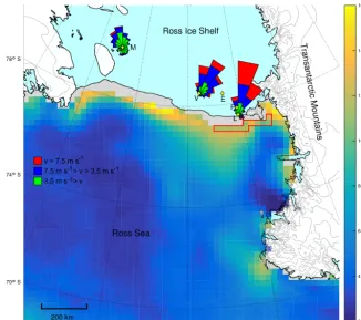
Figure 1.Map of Ross Sea region, grey contour lines indicate topography at 500 m intervals (Liu et al., 2001). The color scale indicates the standard deviation of bootstrap SIC for 20 April–1 November 1979–2014. Yellow diamonds indicate the positions of Margaret, Vito, Emilia, Ferrell and Laurie II AWS sites, labeled M, V, E, F and L, respectively. Wind roses for Margaret, Vito and Laurie II are included. The green, blue and red colors indicate the low, medium and high wind speeds based on the 33rd and 66th percentile wind speeds (3.5 and 7.5 ms−1) as measured at Laurie II. The red line outline indicates the region discussed in Sect. 2.
Figure 1 shows the standard deviation of SIC, calculated from the daily variation from the long-term winter mean of bootstrap SIC data over the period 20 April until the 1 November for the years 1979 until 2014. This period was chosen to exclude the annual break out of sea ice to minimize variability not associated with day-to-day polynya activity. Coastal pixels often display a large variability, for example the area longitude 170 and 180◦E extending several hundred kilometers offshore. The orientation of this area corresponds well with both the dominant wind directions observed at the Laurie II AWS site and the location of the RSP as identi-fied in Nakata et al. (2015) amongst others. Large deviations from the mean are due to the high variability in SIC within the polynya, as displayed in Fig. 2.
For our analysis we define a region comprised of pixels adjacent to the bootstrap land mask and 10◦wide in longitude centered on the Laurie II AWS site, identified in red in Fig. 1. This gives a 25 km by 250 km region close to the Ross Ice Shelf and Ross Island, colocated within the area where the Ross Sea polynya can be observed. The wind roses in Fig. 1 display the distribution of wind vectors observed at various AWS sites (Margaret, Vito and Laurie II).
We derive sea ice motion vectors from the National Snow and Ice Data Center’s 12.5 km resolution polar stereographic gridded brightness temperatures, retrieved from the special sensor microwave/imager and special sensor microwave im-ager/sounder (SSMIS) instruments (Maslanik and Stroeve, 2004). Daily averages are available from July 1987 to De-cember 2015. We utilize the vertical and horizontal polar-izations of the 85.5 GHz channel from 1987 to 2009 and the 91.7 GHz channel from 2010 onwards.
Following multiple authors (Emery et al., 1997; Heil et al., 2006; Holland and Kwok, 2012), we estimate ice motion via a maximum cross-correlation method. We track 9×9 grids of stereographic cells (112.5×112.5 km) over a radius of eight grid cells (100 km). The search radius provides an up-per limit for ice velocity of approximately 1.2 ms−1, defining a physically plausible range (Heil et al., 2006).
Time of year
January February March April May June July August September October November December
Sea ice concentration [%]
0 10 20 30 40 50 60 70 80 90
100 Mean sea ice area 1988–2014
Time of year
January February March April May June July August September October November December
Sea ice concentration [%]
0 10 20 30 40 50 60 70 80 90
100 Sea ice area 2013
(a)
(b)
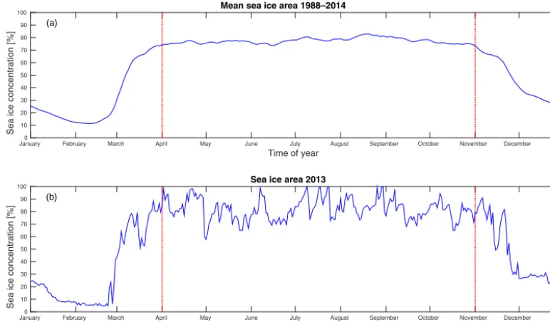
Figure 2. (a)Mean SIC within RSP north of the Laurie AWS from the region identified in Fig. 1.(b)SIC during 2013, highlighting day-to-day variability. Red dotted lines identify the period from April to October used in this study.
uses the maximum correlation from both the horizontal and vertical polarizations. From the resulting displacement and time period the ice velocity was estimated. We subsequently smoothed the gridded velocities to a 25 km stereographic grid.
Using this simple method, fast small-scale motions as well as rotations and divergence of the ice pack are not resolved. Furthermore, motion in coastal areas is likely to be less ac-curate due to the difficulties in applying the method to in-complete grids. Brightness temperature-derived motions are considered inaccurate outside of the winter season due to sur-face melt and high levels of atmospheric water vapor (Emery et al., 1997; Holland and Kwok, 2012). Hence, we restrict our analysis of sea ice motions to the cold months of April to October.
We compare winds observed at the AWS sites with 10 m winds of the ERA-interim meteorological reanalysis model (Dee et al., 2011). The model output is available on a 0.75◦×0.75◦grid at a 6 h temporal resolution running from late 1979 until present. Although AMPS provides higher-resolution weather data, ERA-Interim was used due to its temporal consistency and data set spanning the AWS period. ERA-interim does not assimilate wind speed measurements over land (including ice shelves) and is therefore indepen-dent from AWS measurements. For comparison of AWS and ERA-interim wind data, virtual AWSs were created by in-terpolating the wind speed from the ERA-Interim grid to the location of the AWS sites using a bilinear interpolation.
3 Results
3.1 SIC within the Ross Sea polynya
Figure 2a shows the mean SIC within the coastal area iden-tified in Fig. 1 averaged over the period 1988 to 2014. Throughout the winter period, defined between 1 April and 1 November in this study, the total SIC within this area is relatively constant. Outside this period we observe a gradual decrease in SIC from November until a minimum is reached in mid-February, followed by a more rapid increase in SIC in early March. For the remainder of this analysis we will only consider the period from April to October to remove the ef-fects of summer melt and to avoid periods with low SIC and large gradients in SIC. Figure 2b shows the daily SIC for the same area derived from data in 2013 to show the high degree of variability in the SIC in this region; these results resem-ble a previous analysis reported in Bromwich et al. (1998). The large day-to-day variability between April and October (Fig. 2b) is likely to be associated with polynya processes. The sawtooth features observed in this specific year, for ex-ample around 1 May, are common features and illustrate that decreases in SIC generally occur more rapidly than the fol-lowing increases in SIC, a point that will be supported by later analysis.
3.2 Inter-comparison of AWS and ERA-Interim wind speeds
histograms indicating prevailing winds; the colors indicate the distribution of wind speed in each angular sector. Inspec-tion of the wind rose closest to Ross Island (Laurie II) shows that the wind in this region is dominated by strong southerly flows. These strong southerly flows are also an important feature of the wind distribution at the other AWS sites dis-played in Fig. 1 but are not observed as frequently. However, as identified previously, the results presented do not change appreciably if data from other AWS sites in the northwestern corner of the Ross Ice Shelf are utilized.
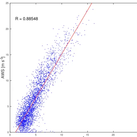
The wind speeds measured at four AWSs, Laurie II, Fer-rell, Emilia and Vito, were compared to the virtual sites in-terpolated from the ERA-Interim model grid. Scalar wind speeds at Laurie II, Ferrell and Emilia correlated well with R2>0.75, while Vito was found to have a weaker corre-lation of R2=0.55. Inspection of ERA-Interim and AWS wind roses revealed no significant directional bias between the two data sets. However, when linear least square fits be-tween the model and the Laurie and Ferrell AWS winds were applied, slopes of 1.70 and 1.52, respectively, were found, indicating that at these sites ERA-Interim generates signifi-cantly weaker wind speeds than measured by the AWS. Scale factors measured at Emilia and Vito were 1.06 and 0.96, re-spectively, indicating a better agreement between the AWS and ERA-Interim wind speeds at these sites. Laurie and Fer-rell are located 36 and 57 km from Cape Crozier (at the eastern end of Ross Island), while Emilia and Vito lie 140 and 223 km east of Ross Island. Thus, the differences ob-served are likely linked to the local topography that is not well represented in the ERA-Interim reanalysis. Recent work by Jolly et al. (2016) comparing AWS observations with the Antarctic Mesoscale Prediction System output (a much higher-resolution atmospheric model) also identifies that the effect of topography in the region can not be reproduced by the model (Powers et al., 2012). It should also be noted that ERA-Interim does not assimilate wind speed measurements over land and so the two data sets are independent (Dee et al., 2011).
3.3 Correlations between SIC and AWS measurements Cross-correlation functions (CCFs) between the time series of SIC within the region in Fig. 1 and both wind speeds and temperatures measured at the Laurie II AWS site were calculated for the 2000–2014 period. For comparison with daily bootstrap SIC data, 24 h running means of the 10 min AWS measurements were used. Although SIC data were only available on a 24 h resolution, wind data were available at a 10 min resolution. By varying the time lag between these two time series and calculating the Pearson correlation coefficient for each lag, CCFs were able to be calculated at a 10 min time resolution. The bootstrap SIC is derived from 24 h binned brightness temperatures and we compared these with the 24 h rolling mean of AWS data. The resulting correlation func-tions will be blurred over a 24 h period. The CCF between
the time series of SIC and both scalar wind speeds and tem-peratures measured at the Laurie II AWS site are shown in Fig. 4.
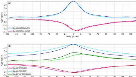
In Fig. 4a we find a strong negative correlation between SIC and wind speed, with the maximum magnitude corre-lation occurring after a 12 h time lag. The minimum is pre-ceded by a rapid decrease and followed by a more gradual in-crease in correlation with respectivee-folding times of−48 and 100 h. This indicates that during high-wind events the SIC in the RSP area is generally low. The difference in the decrease and increasee-folding times suggests that the two changes are controlled by different processes. For example, we expect that the decrease in SIC is dominated by more rapid northward advection, while the increase in SIC during sea ice formation is dominated by slower ice formation. This interpretation is supported by the recent analysis detailed in Nakata et al. (2015), which used a simplified model to under-stand polynya changes.
Laurie II is located about 50 km south of the region used for the SIC analysis. A change of predominantly southerly winds (Parish and Bromwich, 2007) is first observed upwind at Laurie II before the signal propagates to the RSP down-wind. Wind blowing at 5 ms−1would take about 3 h to travel the distance, meaning the 12 h delay observed cannot be en-tirely explained by this process. Another contributing factor is that the region used for calculating the SIC is not directly adjacent to the northern edge of the RIS and an area of sea ice may exist south of the studied polynya area. If a north-ward advection of sea ice occurs, the ice advected from the region will be replaced by ice in the unobserved region be-tween the Ross Ice Shelf and the region specified in Fig. 1. This could allow advection of sea ice to occur for a short period of time without a decrease in SIC occurring, caus-ing the minimum in sea ice to occur several hours after a significant increase in wind speed. In addition, as a strong wind event progresses, the sea ice will ridge and raft upon it-self, causing the surface roughness of the ice to increase. We speculate that this will make the ice slightly more suscepti-ble to the wind stress (Mårtensson et al., 2012). As the SIC decreases, internal stresses prohibiting motion will decrease, allowing advection to become more significant. These effects will cause the minimum SIC to occur slightly after the time of maximum wind speed and are likely causes of the location of the minimum correlation between SIC and wind occurring at approximately a 12 h delay, though the collection of swath data also introduces some uncertainty in the exact timing. Wind speeds in the area autocorrelate with ane-folding time of 36 h (Fig. 4a), which explains the significant correlations in the CCF between AWS wind speed and SIC at negative de-lay. Thee-folding time for the decrease in this CCF is−48 h and the extrema occurs at a delay of 12 h corresponding with the 36 he-folding time for AWS wind speeds.
ERA [m s ]
0 5 10 15 20 25
AWS [m s ]
0 5 10 15 20 25
R = 0.88548
-1
-1
Figure 3.Scatter plot of 24 h mean wind speed for winter 2000– 2014, measured by Laurie II AWS against that of ERA-Interim. The red line indicates the linear least squares fit.
this curve are −120 and 170 h for the decreasing and in-creasing periods, respectively. These values are both similar to the autocorrelation e-folding time for temperatures mea-sured at Laurie II of 150 h. As a strong wind event progresses and SIC decreases, the heat flux from the ocean to the at-mosphere will increase, causing production of new sea ice through freezing. The rate of freezing of open water will de-pend on the temperature differential between the ocean and the atmosphere, potentially explaining the significant corre-lations observed. Significant positive correcorre-lations can also be found between the temperature and wind speeds measured at the Laurie II station (Fig. 4b), which we interpret as at least partially the cause of the correlation between temper-ature and SIC. In addition, work detailed in Coggins et al. (2014) also suggests that strong wind events, particularly Ross Ice Shelf airstream (RAS) events (Parish et al., 2006), are related to warm surface temperature anomalies. This is due to changes in low-level stratification. During periods of low winds, a layer of cool, dense air is observed near the surface, while during higher wind speeds the warmer overly-ing layer is mixed down toward the surface. Adiabatic warm-ing linked to air traverswarm-ing the Transantarctic Mountains also contributes to this temperature anomaly. However, given that the correlation between temperature and wind speed at Lau-rie II is 0.5 at zero hours and the correlation between temper-ature and SIC is−0.65, there must be some other causal link between temperature and SIC. We suggest that this is likely due to a more gradual rate of freezing of open water dur-ing periods of higher air temperatures (effectively a smaller
temperature differential between ocean and air temperatures impacting the sensible heat flux).
3.4 Comparison of ERA-Interim and AWS CCFs CCFs were also produced using the ERA-Interim virtual AWSs in the same manner, although at a 6 h temporal resolu-tion dictated by the temporal resoluresolu-tion of the ERA-Interim output. We found that both the wind speed, SIC and wind speed autocorrelation were very similar to those found using the AWS wind speeds (Fig. 2a). This is not surprising since the ERA-Interim wind speeds correlate well with those of AWS at Laurie. The CCF of temperature versus SIC, CCF of temperature versus wind speed and the temperature auto-correlation from the ERA-Interim output have similar forms to the relationships derived using AWS data but are gener-ally smoother and the magnitude of the largest correlations are generally smaller. The temperature autocorrelation curve shows that ERA-interim predicts more persistent tempera-tures than the Laurie II AWS measures. This likely indicates that high-frequency temperature fluctuations are not accu-rately modeled within ERA-interim. The ERA-Interim CCF of wind speed versus temperature shows weaker correlation for delays less than 24 h, with the difference becoming negli-gible around−72 h. This probably indicates that the warming of the air due to mixing, suggested in Coggins et al. (2013) and other studies, caused by strong winds is underestimated in ERA-interim. These effects likely cause the small differ-ences between the ERA-interim temperature and SIC corre-lations and the correcorre-lations of the Laurie II AWS.
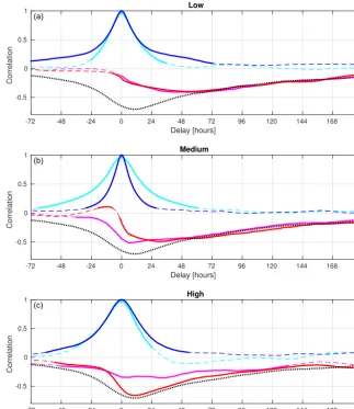
Cross-correlation curves for SIC and wind speed measured at Laurie II AWS site and wind speed hindcast from the ERA-Interim virtual station are now examined (Fig. 5a–c). The daily mean wind speeds measured at Laurie II were catego-rized into low, medium and high-wind events based on 33rd and 66th percentile AWS wind speeds measured at Laurie II (3.5 and 7.6 ms−1, respectively). Wind direction was not con-sidered in this classification because of the predominance of southerly flows at the site. CCFs for SIC with wind speed were calculated only for periods when the mean wind speed during a−12 to+12 h period was within one of the three cat-egories (Fig. 5). Autocorrelation curves for the wind in each of these three cases were also calculated to allow the persis-tence of each of the three strengths of wind speed events to be identified. The AWS medium-wind case autocorrelation curve (Fig. 5b) shows considerably lower persistence than either of the extreme cases, indicating that this is a transition state that occurs frequently for short periods. The high-wind case (Fig. 5c) shows a CCF very similar to that of all cases (Fig. 4b), excluding the period from−36 to+12 h delay.
Delay [hours]
-192 -168 -144 -120 -96 -72 -48 -24 0 24 48 72 96 120 144 168 192
Correlation
-0.8 -0.6 -0.4 -0.2 0 0.2 0.4 0.6 0.8 (a)
AWS wind speed autocorrelation ERA wind speed autocorrelation AWS wind speed, SIC correlation ERA wind speed, SIC correlation
Delay [hours]
-192 -168 -144 -120 -96 -72 -48 -24 0 24 48 72 96 120 144 168 192
Correlation
-0.8 -0.6 -0.4 -0.2 0 0.2 0.4 0.6 0.8 (b)
AWS temp, SIC correlation ERA temp, SIC correlation AWS temp autocorrelation ERA temp autocorrelation AWS temp, wind speed correlation ERA temp, wind speed correlation
Figure 4. (a)Cross-correlation curve for sea ice concentration and AWS (red) and ERA-Interim (magenta) wind speeds and autocorrelation curve for wind speed at Laurie II AWS (blue) and ERA-Interim (cyan).(b)Cross-correlation curve for sea ice concentration and temperature for AWS (red) and ERA-Interim (magenta); autocorrelation curves for wind speed at Laurie II AWS site (blue) and ERA-Interim (cyan) are also shown. Cross correlation for wind speed and temperature measured at Laurie II AWS (dark green) and ERA-Interim (light green). Dashed lines indicate significancep >0.01. The delay is defined such that positive indicates meteorology measures leading SIC.
wind speed. With the exception of a short period in the medium case, spanning−30 to 6 h, when weak positive cor-relations were observed. The medium case has a correlation extrema of−0.5 at 30 h, while the extrema for the low case is
−0.4 at 50 h between AWS and SIC data. Both these values are significantly weaker and later than those of both the high and total cases. This could be because weaker wind speeds will not have as significant of an effect on sea ice, causing any advection of sea ice and subsequent sea ice break up to occur much less rapidly than the high-wind case. Another possible cause is that the higher wind speeds within each class are more likely to increase to stronger cases after the classified period, causing a decrease in SIC at a large delay. Due to the autocorrelation for both medium and low cases being very low at their respective times of extrema, the for-mer explanation seems unlikely since there would be little coherence between wind speed at 0 h and wind speed at the extrema.
The categorized autocorrelation curves found using the ERA-interim virtual station are not as perfectly symmetri-cal as those for the AWS data. This is due to sampling issues that occur at the beginnings and ends of the broken time se-ries, obtained because of the wind speed classifications used. These sampling issues are also present in the AWS autocor-relation curves but are of greater significance when using
the low-temporal-resolution ERA-interim data. The medium ERA-interim wind speed autocorrelation curve shows persis-tence similar to that of the low and high cases, differing from that of AWS, which showed a much shorter persistence in the medium case. In the low-wind case, CCF of wind speed ver-sus SIC derived from ERA-interim output is very similar to that found using AWS. In contrast, the ERA-interim CCFs in the medium- and high-wind-speed cases differ significantly from those of AWS. In particular, the ERA-interim medium case displays stronger negative correlations than that of the AWS between−24 and 24 h, after which the two are very similar. The high-wind regime for ERA-Interim displays sig-nificantly weaker correlations between −12 and 72 h than the corresponding pattern derived using AWS data. The lat-ter point likely reflects the fact that the ERA-Inlat-terim data are generally poor at representing the strength of the wind in the strong-wind-speed periods for this region, this being sup-ported by the large gradient derived (1.70) when applying a linear least squares regression to the ERA-Interim and AWS wind speeds.
3.5 SIC anomalies during extreme wind events
Delay [hours]
-72 -48 -24 0 24 48 72 96 120 144 168 192
Correlation
-0.5 0 0.5 1
(a)
Low
Delay [hours]
-72 -48 -24 0 24 48 72 96 120 144 168 192
Correlation
-0.5 0 0.5 1
(b)
Medium
Delay [hours]
-72 -48 -24 0 24 48 72 96 120 144 168 192
Correlation
-0.5 0 0.5 1
(c)
High
Figure 5.Cross-correlation curves for SIC and AWS (red) and ERA-Interim (magenta) wind speeds at the Laurie II AWS site for periods of low(a), medium(b)and high(c)winds. Wind autocorrelation curves for low-, medium- and high-wind cases from AWS (blue) and ERA-Interim (cyan). Dashed lines indicate significancep >0.01. The dotted black line represents the cross-correlation curve for the total of all wind cases for comparison.
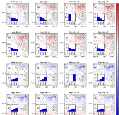
the SIC anomalies for the high- and low-wind classes previ-ously identified for different periods relative to the onset of those classes. For both low- and high-wind classes, the April to October mean bootstrap SIC anomaly for each pixel in the Ross Sea region was calculated over the 2001–2014 period (defined by Laurie II AWS coverage) (Fig. 6). Composites for several days of delay before and after the wind event on-set were then derived to highlight how the sea ice anomaly varies spatially prior to and following these wind classes. Histograms are also shown to indicate how the distribution of each wind class changes throughout the period examined. On day zero all cases are either 100 % high or low winds, but on following days the winds are not classified. This allows the persistence of these wind events to be observed. We find significant, positive anomalies within the Ross Sea polynya during low winds and negative anomalies during high winds
Figure 6.Composites of 2000–2014 sea ice concentration anomaly at varying delay for low-wind cases(a–h)and high-wind cases(i–p). The grey and black contours indicate 80 and 99 % significance, respectively. The inset histograms indicate the percentage of the three wind cases that occur at the respective delay.
3.6 Sea ice motion anomalies during extreme wind events
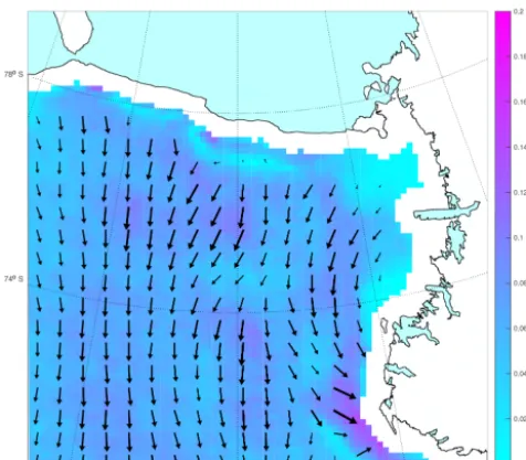
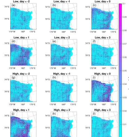
The mean sea ice motion vectors for April–October 2001 un-til 2014 (Fig. 7) show northward flow throughout the Ross Sea, with an easterly component occurring to the east of Cape Adare. This highlights the net export of sea ice from the north-facing coasts of the Ross Sea throughout this period (Comiso et al., 2011). Composites of sea ice motion anoma-lies related to high- and low-wind states at delays varying from −2 to 3 days from the wind event are displayed in Fig. 8. During periods of low wind speed at Laurie II, anti-cyclonic anomalies occur throughout the Ross Sea (Fig. 8a– f). Conversely, cyclonic anomalies are found during periods of high winds at Laurie II (Fig. 8g–l). These anomalies are largest at zero lag but persist for 24 h after the wind event,
with weak anomalies being found in both low and high states 48 h after the wind event. It is also noticeable that no coherent pattern in the sea ice anomalies associated with the medium-wind state are observed (not shown). The cyclonic anomalies during strong wind events and anticyclonic anomalies dur-ing low-wind events highlight the critical influence of atmo-spheric near-surface winds on sea ice motion in the region.
4 Discussion
Figure 7.Mean sea ice motion vectors in the Ross Sea region. Ar-rows indicate the mean sea ice drift vector over a 100×100 km region. The color scale indicates the magnitude of this vector field.
from the shore than the one used in our analysis. Winds over the Bromwich RSP area were not as well represented by the Ferrell AWS, explaining the weaker correlations. We found a minimum correlation between Ferrell wind speed and SIC to be−0.72 at a 10 h delay; Bromwich et al. (1998) did not cal-culate correlations at varying delay, making comparison with this value impossible. Bromwich et al. (1998) also found cor-relations between SIC and inverse temperature ranging be-tween 0.44 and 0.55. We found a correlation of 0.64 bebe-tween SIC and inverse temperature; this difference is due to the dif-ferent RSP area and time periods used.
ERA-Interim was able to generate wind speeds that cor-related well with those of several AWS sites, indicating that the relative wind speeds within ERA-Interim were consistent with the AWS measurements. However, at AWS sites near significant topography, ERA-Interim was found to predict wind speeds significantly weaker than the winds measured by the AWS, with slopes of the regression lines of 1.70 and 1.52 (implying that the ERA-Interim values are this factor smaller than the AWS measurement) at the Laurie II and Ferrell sites, respectively (Fig. 3). This is likely because ERA-Interim is unable to accurately model the mesoscale barrier affect of Ross Island and the resulting flow convergence. This hypoth-esis is supported by recent comparisons between AWS data and mesoscale model output in the region (Jolly et al., 2016). The CCF of wind speed versus SIC produced using the vir-tual Laurie station was very similar to that found using the Laurie AWS data. However, when the data were separated into low-, medium- and high-wind regimes, based on a cate-gorization derived from the AWS data, significant differences were found between the ERA-Interim and AWS CCFs. This suggests that the ERA-Interim output provides a good
repre-sentation of the occurrence of the different wind states, but the magnitudes from the ERA-Interim underestimate the val-ues observed by AWS. This indicates that ERA-Interim out-put is not be a reliable way to identify relevant wind thresh-olds used in models simulating polynya dynamics. This fac-tor makes the usage of ERA-Interim problematic for polynya studies since they generally form on coastlines near topogra-phy in Antarctica. ERA-Interim provides 10 m wind speeds, while the AWS wind speeds are measured at 2–3 m (Lazzara et al., 2012; Dee et al., 2011). This would suggest that a scale factor exists between the two data sets, an effect that was not corrected. While this will not affect the correlation compar-isons performed, it may explain the scale factors observed. However, this small height difference is not able to explain the large-scale factors found, indicating that topography must have a significant effect.
Sea ice motion vector anomaly composites indicate that wind-driven sea ice drift is significant 12 h before through to 36 h after strong wind events peak. This coincides with the peak cross correlation between SIC and wind speed, indicat-ing that durindicat-ing a strong wind event, SIC within the RSP is at a minimum during the period where wind-driven sea ice drift is found to be significant. Following strong wind events, significant negative SIC anomalies are also found and per-sist for up to 5 days after the event. This period is longer than the persistence of most strong wind events (see auto-correlation in Figs. 4 and 5), and it therefore seems unlikely that the SIC recovery following strong wind events is con-trolled by wind-driven advection of sea ice. Thus, the re-covery of sea ice is likely dominated by formation of new sea ice within the RSP rather than advection of existing sea ice, an assumption supported by recent analysis detailed in Nakata et al. (2015). During periods of high wind, negative SIC anomalies were found within the Ross Sea polynya. Sim-ilarly, positive anomalies were found during periods of low wind. The significant anomalies were also only found within areas of known polynyas, likely due to thinner, less concen-trated sea ice being present within the polynyas. Correlations between wind speed and SIC were significantly stronger for the high-wind class than the two weaker classes (Fig. 5), in-dicating that the wind-driven polynya mechanism is driven by the strongest wind speeds and moderate winds have a less significant effect.
Figure 8. (a–f)Sea ice motion anomalies for days−2 to 3 for low-wind events.(g–l)Sea ice motion anomalies for days−2 to 3 for high-wind events. Composites are formed over the 2000–2014 period.
Transantarctic Mountains and a semi-persistent low-pressure system east of the Ross Sea. This was also identified in detail analysis around the Laurie II region presented in Jolly et al. (2016). This directional bias becomes even stronger when only the largest wind speeds are considered. This means that errors due to northerly winds are minimal in our analysis.
Only the results obtained from weather data taken at Lau-rie II are presented in this study because of its proximity to the RSP. However, a similar set of analyses were performed for the Vito, Emilia, and Ferrell AWS sites. These produced similar results, with the only significant difference being that weaker correlations were found at these sites when compared to those with Laurie II. This is hypothesized to be because
these sites are based further inland, and are therefore more distant from the center of the RSP than Laurie II. This would mean that the winds at these locations would be less repre-sentative than those at Laurie II.
winds to be observed within the RSP. Meanwhile, other areas of the RSP north of Ross Island will be somewhat sheltered from many of the predominant southerly winds. Due to the relatively warm ocean, an upward heat flux will occur within the RSP when open water or thin ice is present. This will cause an increase in surface air temperatures over the RSP. This effect will not occur at Laurie II due to the insulation of the thick ice shelf. Due to the lack of measurements within the RSP, the net result of these effects is unidentifiable.
When within 50 km of the coastline, the sea ice motion vectors used in this study are biased. This coastal area co-incides with the majority of polynya activity and therefore the dynamic effects of changing wind speeds were not able to be observed directly within the RSP. The assumption is made that offshore sea ice drift will be representative of drift in coastal polynyas. Although derived sea ice motion is co-herent throughout the Ross Sea, the motion within coastal polynyas may be different since thinner, less concentrated ice exists within coastal polynyas.
The bootstrap SIC data used throughout this study use passive microwave measurements to calculate SIC. The mi-crowave signature for a thin sheet of ice can be identical to that of scattered thick ice. For sea ice thickness less than 10 cm, the bootstrap sea ice concentration is a function of sea ice thickness (Kwok et al., 2007). During periods of low wind speed, bootstrap SIC within the RSP often reaches 100 %, in-dicating a continuous covering sheet of sea ice with thickness greater than 10 cm. During a strong wind event, the SIC de-creases via dynamic processes, leaving areas of open water with scattered, likely thick ice. As freezing of the open water occurs, a layer of thin ice will form, causing a gradual in-crease in the bootstrap SIC. As this sea ice thickens, the heat flux between the warmer ocean and the cooler atmosphere will decrease, causing the rate of freezing to also decrease. Because both bootstrap SIC and the rate of freezing within a polynya depend on the thermal conductivity of the sea ice, the bootstrap SIC may actually provide a more meaningful measure of sea ice production within polynyas than true SIC values.
Despite the length of the bootstrap SIC time series, we were unable to identify any significant trends in polynya ac-tivity. This may be due to changing polynya structure as a re-sult of calving from the Ross Ice Shelf and the ice shelf grad-ually advancing northward. As the coastline evolves, so does the RSP. This causes issues since the land mask for bootstrap SIC data does not change with time. Over long periods, a changing amount of the RSP is visible in the bootstrap SIC data, causing biases in any metric for polynya activity. This effect was particularly obvious in 2005 when iceberg B15 calved from the Ross Ice Shelf, moving a 300 km long sec-tion of the northern coastline 40 km further south.
5 Conclusions
During the austral winter, strong negative correlations were found between AWS wind speeds and SIC in the RSP. In contrast to previous studies, we examined these correlations as a function of lag and found that they persisted for several days and exceeded the persistence of the wind speed auto-correlation. When the data were split into low-, medium- and high-wind cases and correlations were calculated from the separate data sets, the high-wind states displayed stronger correlations than the other two states, indicating that stronger winds had the most significant impact on sea ice within the RSP. This analysis was repeated using a virtual AWS site in-terpolated from ERA-Interim reanalysis wind fields. It was found that although strong correlations existed between the AWS and ERA-Interim wind speeds, a linear scale factor, significantly greater than 1 was present at AWS sites in close proximity to topography. Wind speeds measured at the Lau-rie II AWS correlated strongly with colocated ERA-Interim wind speeds, but a scale factor of 1.70 (indicating AWS wind speeds were 1.70 times faster than ERA-Interim wind speeds) was found. The ERA-Interim wind speeds were used to calculate a wind speed against SIC CCF that agreed with the CCF formed using AWS wind speeds. However, when the data set was categorized into low-, medium- and high-wind cases and individual CCFs were calculated, significant dif-ferences from the AWS CCFs were found in the high-wind state. Likely due to the effects of nearby small-scale topog-raphy, ERA-Interim wind speeds were unable to reproduce the relationships found between AWS wind speeds and SIC in the RSP. This difference has implications for interpreting sea ice anomalies using ERA-Interim winds in regions close to complex topography.
impacts on polynya processes, potentially strongly impact-ing coastal sea ice production. This study shows that coarse resolution atmospheric reanalysis data would not capture the correct magnitude of this effect.
6 Data availability
Due to their large size, the sea ice motion vectors used in this study are available upon request.
The AWS data used were accessed via
http://amrc.ssec.wisc.edu/aws/index.php?region=
RossIslandVicinity&station=Laurie0II (Lazzara et al., 2012).
The Bootstrap SIC data used were accessed via the NSIDC website (https://nsidc.org/data/NSIDC-0079/ versions/2#) (Comiso et al., 2008).
Acknowledgements. We would like to thank the support of the University of Wisconsin-Madison Automatic Weather Station Program for the AWS observational data set (NSF grant numbers ANT-0944018, ANT-1245663, ANT-0943952 and ANT-1245737). We would also like to acknowledge the NSIDC for the provision of the SSM/I data set. This work was partially funded by a grant from the New Zealand Antarctic Research Institute, scholarships from both the Department of Physics and Astronomy at the University of Canterbury and NZ Post (administered by Antarctica New Zealand).
Edited by: C. Haas
Reviewed by: three anonymous referees
References
Bintanja, R., van Oldenborgh, G. J., Drijfhout, S. S., Wouters, B., and Katsman, C. A.: Important role for ocean warming and increased ice-shelf melt in Antarctic sea-ice expansion, Nat. Geosci., 6, 376–379, doi:10.1038/ngeo1767, 2013.
Bromwich, D., Liu, Z., Rogers, A. N., and Van Woert, M. L.: Winter atmospheric forcing of the Ross Sea Polynya, in: Ocean, ICE, At-mos. Interact. Antarct. Cont. MARGIN, vol. 75, 101–133, Amer-ican Geophysical Union, doi:10.1029/AR075p0101, 1998. Brümmer, B. and Hoeber, H.: A mesoscale cyclone over the Fram
Strait and its effects on sea ice, J. Geophys. Res.-Atmos., 104, 19085–19098, doi:10.1029/1999JD900259, 1999.
Brümmer, B., Schröder, D., Müller, G., Spreen, G., Jahnke-Bornemann, A., and Launiainen, J.: Impact of a Fram Strait cy-clone on ice edge, drift, divergence, and concentration: Possibil-ities and limits of an observational analysis, J. Geophys. Res., 113, C12003, doi:10.1029/2007JC004149, 2008.
Coggins, J., McDonald, A. J., Plank, G., Pannell, M., Jolly, B., Par-sons, S., and Delany, T.: SNOW-WEB: a new technology for Antarctic meteorological monitoring, Antarct. Sci., 25, 583–599, doi:10.1017/S0954102013000011, 2013.
Coggins, J. H. J., McDonald, A. J., and Jolly, B.: Synoptic clima-tology of the Ross Ice Shelf and Ross Sea region of Antarctica: k -means clustering and validation, Int. J. Climatol., 34, 2330– 2348, doi:10.1002/joc.3842, 2014.
Comiso, J. C.: Bootstrap Sea Ice Concentrations from Nimbus-7 SMMR and DMSP SSM/I-SSMIS, Version 2., Boulder, Color. USA. NASA Natl. Snow Ice Data Cent. Distrib. Act. Arch. Cen-ter., doi:10.5067/J6JQLS9EJ5HU, 2000.
Comiso, J. C. and Nishio, F.: Trends in the sea ice cover using en-hanced and compatible AMSR-E, SSM/I, and SMMR data, J. Geophys. Res., 113, C02S07, doi:10.1029/2007JC004257, 2008. Comiso, J. C., Kwok, R., Martin, S., and Gordon, A. L.: Variability and trends in sea ice extent and ice production in the Ross Sea, J. Geophys. Res., 116, C04021, doi:10.1029/2010JC006391, 2011. Dee, D. P., Uppala, S. M., Simmons, A. J., Berrisford, P., Poli, P., Kobayashi, S., Andrae, U., Balmaseda, M. A., Balsamo, G., Bauer, P., Bechtold, P., Beljaars, A. C. M., van de Berg, L., Bid-lot, J., Bormann, N., Delsol, C., Dragani, R., Fuentes, M., Geer, A. J., Haimberger, L., Healy, S. B., Hersbach, H., Hólm, E. V., Isaksen, L., Kållberg, P., Köhler, M., Matricardi, M., McNally, A. P., Monge-Sanz, B. M., Morcrette, J.-J., Park, B.-K., Peubey, C., de Rosnay, P., Tavolato, C., Thépaut, J.-N., and Vitart, F.: The ERA-Interim reanalysis: configuration and performance of the data assimilation system, Q. J. Roy. Meteor. Soc., 137, 553–597, doi:10.1002/qj.828, 2011.
Drucker, R., Martin, S., and Kwok, R.: Sea ice production and ex-port from coastal polynyas in the Weddell and Ross Seas, Geo-phys. Res. Lett., 38, L17502, doi:10.1029/2011GL048668, 2011. Emery, W. J., Fowler, C. W., and Maslanik, J. A.: Satellite-derived maps of Arctic and Antarctic sea ice motion: 1988 to 1994, Geo-phys. Res. Lett., 24, 897–900, doi:10.1029/97GL00755, 1997. Heil, P., Fowler, C., and Lake, S.: Antarctic sea-ice velocity
as derived from SSM/I imagery, Ann. Glaciol., 44, 361–366, doi:10.3189/172756406781811682, 2006.
Holland, P. R.: The seasonality of Antarctic sea ice trends, Geophys. Res. Lett., 41, 4230–4237, doi:10.1002/2014GL060172, 2014. Holland, P. R. and Kwok, R.: Wind-driven trends in Antarctic
sea-ice drift, Nat. Geosci., 5, 1–8, doi:10.1038/ngeo1627, 2012. Jolly, B., McDonald, A. J., Coggins, J. H. J., Cassano, J.,
Laz-zara, M., Zawar-Reza, P., Graham, G., Plank, G., Petterson, O., and Dale, E.: A validation of the Antarctic Mesoscale Prediction System using Self-Organizing Maps and high density observa-tions from SNOWWEB, Mon. Weather Rev., 144, 3181–3200, doi:10.1175/MWR-D-15-0447.1, 2016.
Kwok, R. and Comiso, J. C.: Spatial patterns of variability in Antarctic surface temperature: Connections to the Southern Hemisphere Annular Mode and the Southern Oscillation, Geo-phys. Res. Lett., 29, 50–1–50–4, doi:10.1029/2002GL015415, 2002.
Kwok, R., Comiso, J. C., Martin, S., and Drucker, R.: Ross Sea polynyas: Response of ice concentration retrievals to large areas of thin ice, J. Geophys. Res., 112, C12012, doi:10.1029/2006JC003967, 2007.
Lazzara, M. A., Weidner, G. A., Keller, L. M., Thom, J. E., and Cassano, J. J.: Antarctic Automatic Weather Station Program: 30 Years of Polar Observation, B. Am. Meteorol. Soc., 93, 1519– 1537, doi:10.1175/BAMS-D-11-00015.1, 2012.
Liu, H., Jezek, K., Li, B., and Zhao., Z.: Radarsat Antarctic Map-ping Project Digital Elevation Model, Version 2., Boulder, Color. USA. NASA Natl. Snow Ice Data Cent. Distrib. Act. Arch. Cen-ter., 2001.
multi-category sea ice model, J. Geophys. Res.-Ocean., 117, C00D15, doi:10.1029/2010JC006936, 2012.
Maslanik, J. and Stroeve, J.: DMSP SSM/I-SSMIS Daily Polar Gridded Brightness Temperatures, Version 4., Boulder, Colorado USA. NASA National Snow and Ice Data Center Distributed Ac-tive Archive Center, doi:10.5067/AN9AI8EO7PX0, 2004. Nakata, K., Ohshima, K. I., Nihashi, S., Kimura, N., and Tamura,
T.: Variability and ice production budget in the Ross Ice Shelf Polynya based on a simplified polynya model and satel-lite observations, J. Geophys. Res.-Ocean., 120, 6234–6252, doi:10.1002/2015JC010894, 2015.
Nicolas, J. P. and Bromwich, D. H.: New Reconstruction of Antarctic Near-Surface Temperatures: Multidecadal Trends and Reliability of Global Reanalyses, J. Climate, 27, 8070–8093, doi:10.1175/JCLI-D-13-00733.1, 2014.
Ohshima, K. I., Fukamachi, Y., Williams, G. D., Nihashi, S., Roquet, F., Kitade, Y., Tamura, T., Hirano, D., Herraiz-Borreguero, L., Field, I., Hindell, M., Aoki, S., and Wakatsuchi, M.: Antarctic Bottom Water production by intense sea-ice for-mation in the Cape Darnley polynya, Nat. Geosci., 6, 235–240, doi:10.1038/ngeo1738, 2013.
Parish, T. R. and Bromwich, D. H.: Reexamination of the Near-Surface Airflow over the Antarctic Continent and Implications on Atmospheric Circulations at High Southern Latitudes, Mon. Weather Rev., 135, 1961–1973, doi:10.1175/MWR3374.1, 2007. Parish, T. R., Cassano, J. J., and Seefeldt, M. W.: Characteristics of the Ross Ice Shelf air stream as depicted in Antarctic Mesoscale Prediction System simulations, J. Geophys. Res., 111, D12109, doi:10.1029/2005JD006185, 2006.
Powers, J. G., Manning, K. W., Bromwich, D. H., Cassano, J. J., and Cayette, A. M.: A Decade of Antarctic Science Sup-port Through Amps, B. Am. Meteorol. Soc., 93, 1699–1712, doi:10.1175/BAMS-D-11-00186.1, 2012.
Reddy, T. E., Arrigo, K. R., and Holland, D. M.: The role of thermal and mechanical processes in the formation of the Ross Sea summer polynya, J. Geophys. Res., 112, C07027, doi:10.1029/2006JC003874, 2007.
Sen Gupta, A. and England, M. H.: Coupled Ocean–Atmosphere– Ice Response to Variations in the Southern Annular Mode, J. Cli-mate, 19, 4457–4486, doi:10.1175/JCLI3843.1, 2006.
Stammerjohn, S. E., Martinson, D. G., Smith, R. C., Yuan, X., and Rind, D.: Trends in Antarctic annual sea ice retreat and advance and their relation to El Niño – Southern Oscillation and South-ern Annular Mode variability, J. Geophys. Res., 113, C03S90, doi:10.1029/2007JC004269, 2008.
Tamura, T., Ohshima, K. I., and Nihashi, S.: Mapping of sea ice production for Antarctic coastal polynyas, Geophys. Res. Lett., 35, L07606, doi:10.1029/2007GL032903, 2008.
Turner, J., Comiso, J. C., Marshall, G. J., Lachlan Cope, T. A., Bracegirdle, T., Maksym, T., Meredith, M. P., Wang, Z., and Orr, A.: Non annular atmospheric circulation change induced by stratospheric ozone depletion and its role in the recent increase of Antarctic sea ice extent, Geophys. Res. Lett., 36, L08502, doi:10.1029/2009GL037524, 2009.
Turner, J., Hosking, J. S., Bracegirdle, T. J., Marshall, G. J., and Phillips, T.: Recent changes in Antarctic Sea Ice, Philos. T. Roy. Soc. A, 373, 20140163, doi:10.1098/rsta.2014.0163, 2015. Whitworth, I. and Orsi, A. H.: Antarctic Bottom Water production