www.nonlin-processes-geophys.net/17/329/2010/ doi:10.5194/npg-17-329-2010
© Author(s) 2010. CC Attribution 3.0 License.
Nonlinear Processes
in Geophysics
Spatio-temporal error growth in the multi-scale Lorenz’96 model
S. Herrera1, J. Fern´andez1, M. A. Rodr´ıguez2, and J. M. Guti´errez2
1University of Cantabria, Department of Applied Mathematics, 39005 Santander, Spain 2Instituto de F´ısica de Cantabria, CSIC-UC, 39005 Santander, Spain
Received: 19 June 2009 – Revised: 1 July 2010 – Accepted: 3 July 2010 – Published: 22 July 2010
Abstract. The influence of multiple spatio-temporal scales
on the error growth and predictability of atmospheric flows is analyzed throughout the paper. To this aim, we consider the two-scale Lorenz’96 model and study the interplay of the slow and fast variables on the error growth dynamics. It is shown that when the coupling between slow and fast vari-ables is weak the slow varivari-ables dominate the evolution of fluctuations whereas in the case of strong coupling the fast variables impose a non-trivial complex error growth pattern on the slow variables with two different regimes, before and after saturation of fast variables. This complex behavior is analyzed using the recently introduced Mean-Variance Log-arithmic (MVL) diagram.
1 Introduction
The growth of perturbations, or errors, in weather or climate models has been discussed in the literature from different points of view using both simplified “toy” models (Guti´errez et al., 2008) and real operational systems (Fern´andez et al., 2008). A common behavior has been identified in these cases. When plotting in a diagram the variance against the mean of the logarithms of perturbations (the so called Mean-Variance Logarithmic (MVL) diagram) a typical trajectory appears as the fingerprint of the spatio-temporal dynamics of the perturbations. These MVL trajectories usually show two distinct regimes. The first, with increasing variance, has been identified as a genuine infinitesimal fluctuation where the in-creasing variance appears as a result of the collapse to the main Liapunov vector. The second, showing a decrease of variance, appears by nonlinear effects (hence it is a genuine finite fluctuation) that destroy the spatial correlation and lo-calization of the perturbations (Primo et al., 2007; Guti´errez
Correspondence to: S. Herrera
et al., 2008). Hence, this methodology allows the charac-terization of both the temporal and spatial growth compo-nents, and their interplay, explaining the characteristic local-ized structure of error growth.
In all cases analyzed until now with this methodology, the system had a single temporal scale, and so these studies did not clearly establish the role of the multiple scales existing in the atmosphere. Moreover, little is known about the behavior with more temporal scales. This study is interesting from both fundamental and applied points of view. Many basic questions about the meaning and generation of infinitesimal and finite perturbations in models with multiple scales still remain open. Also, questions of practical interest such as the way of initializing ensembles with coupled ocean atmo-sphere models are unsolved.
This paper addresses the role of the multiple scales in the dynamics of the perturbation growth. A new complex growth pattern with several regimes of evolution is shown and analyzed. In Sect. 2 we describe the one- and two-scale Lorenz’96 models comparing their behavior. In Sect. 3 a quantitative description of the growth patterns obtained in one-scale L96 model is presented. Section 4 analyzes the growth of perturbations in the two-scale L96 model. Finally, some conclusions are given in Sect. 5.
2 The two-scale Lorenz’96 model
The Lorenz’96 system (L96) is a simple conceptual model of atmosphere-like multi-scale dynamics (Lorenz, 1996). It consists ofmslow variablesxicoupled tom×nfast variables
yj,i whose evolution is governed by the following nonlinear
equations modeling advection, constant forcing, and linear damping:
dxi
dt =xi−1(xi+1−xi−2)−xi+F− hc
b
n X
x1
x2
y y1,1 4,1
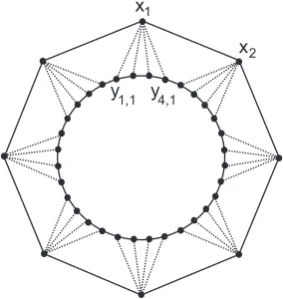
Fig. 1. Schematic illustrations of the L96 system withm=8 and
n=4, with a total ofm×ngrid points in the inner circle.
dyj,i
dt =cbyj+1,i yj−1,i−yj+2,i
−
cyj,i+
hc
b xi, (1) wherei=1,...,m,j=1,...,n;his the coupling constant,b andcare the scaling constants andF is a constant forcing. Both thexi’s and theyj,i’s are assumed to be periodic, i.e.,
xm+1=x1;x0=xmandyn+1,i=y1,i+1;y0,i=yn,i−1. L96 was originally introduced to mimic multi-scale mid-latitude weather, considering an unspecified scalar meteorological quantity atmequidistant grid points along a latitude circle (see Fig. 1); moreover, each of these points was associated withn fast variables providing a higher resolution descrip-tion of the system (m×ngrid points).
In this paper we considered the conventional parameter values F=8 and m=40. This leads to a chaotic behavior with a time unit corresponding approximately to five days in an equivalent atmospheric model (Lorenz, 1996). This is the time unit used throughout the paper. We also selected n=4, b=10 andc=10, leading to a two-scale model where the fast variables fluctuate 10 times faster than the slow ones, but with a smaller amplitude. The coupling parameterhcan be varied in the range (0, 1) to obtain different degrees of coupling between both scales. This model has been exten-sively used in the literature to study the influence of mul-tiple spatio-temporal scales on the predictability of atmo-spheric flows. For instance, Wilks (2005) studied stochastic parametrization, Lorenz and Emanuel (1998) analyzed tar-geted observations and Orrell (2003) predictability over dif-ferent timescales.
A simplified version of L96 has also been used to investi-gate the dynamics of the slow variables alone. In this case, the system is given by:
dzi
dt =zi−1(zi+1−zi−2)−zi+F . (2) Both systems were integrated using a fourth-order Runge-Kutta method with dt=0.005.
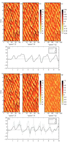
Figure 2a shows trajectories obtained by integrating (2) from a random initial conditionzi(0). After a short transient
these figures show the typical pattern of L96 model emulat-ing atmospheric flows: waves with mean length of 5 units travel westward in a noisy background induced by chaos spending 7–9 time units to complete a latitude circle. Fig-ure 2b and c shows the trajectory for the two-scale model (1) integrated from a random initial condition(xi(0),yj,i(0))=
(zi(0),yj,i(0))and weak coupling (h=0.3) Thezi andxi
tra-jectories are initially very close, but they diverge very soon due to non-linear behavior and the effect of the fast variable dynamics. Contrarily, the spatial patterns of the X and Y trajectories are, after rescaling, very similar at all times. Fig-ure 2f and g shows the trajectories of the two-scale model with the same initial conditions but with a stronger coupling (h=1). The main difference with the previous case can be seen in the fast variable, that now exhibits a high variability at small scales. In order to appreciate this fact we plot in Fig. 2d and h the trajectories of a reference pointx1,y1,1and the coupling termS1=cPnj=1yj,1. Note that this latter term is the true contribution, as an additive source, of the fast vari-ables to the slow ones at a given pointi=1. Figure 2d shows that with weak coupling the dynamics of the fast variable is conditioned by the slow variable. It is a coupling dominated by the slow dynamics. Figure 2h shows the opposite effect, clearly the dynamics is dominated by fast variables. This ef-fect is seen as producing high frequency spatial and temporal structures.
In all cases the last time step of this trajectory was used as the initial condition in the following section, in order to have a flow-assimilated initial condition.
3 Spatio-temporal growth of perturbations in one-scale
systems
In this section we describe the growth of perturbations (e.g., errors in the initial conditions) in a one-scale system such as the one generated by Eq. (2). First, we show a qualita-tive description showing the phenomena of spatial localiza-tion and saturalocaliza-tion. Then, we present a more quantitative de-scription taking logarithms of the absolute perturbations and using the MVL diagram to obtain the characteristic curve for the spatio-temporal error growth.
3.1 Qualitative description
Let us consider a perturbed trajectory around a control fore-castzi(t )for the one-scale L96 model, which is computed
integrating (2) from a flow-assimilated initial conditionzi(0)
(see previous section). The perturbed trajectory corresponds to the integration forward in time of the perturbed initial conditionz0i(0)=zi(0)+δzi(0), whereδzi(0)are
1 2 3 4 5 6 7 8 9 10 −15
−10 −5 0 5 10 15 20
1 2 3 4 5 6 7 8 9 10
−15 −10 −5 0 5 10 15 20
Xi Si Yj,i
Xi Si Yj,i 12
6
-6 -8 4 10 8
2 0 -2 -4
10 9 8 7 6 5 4 3 2 1 0
time
1 10 20 30 40 “space”: Zi
1 10 20 30 40 “space”: Xi
0.36
0.18
-0.18 -0.24 0.12 0.3 0.24
0.6 0 -0.6 -0.12
1 40 80 120 160 “space”: Yj,i
12
6
-6 -8 4 10 8
2 0 -2 -4
1 10 20 30 40 “space”: Xi
1.2
0.6
-0.6 -0.8 0.4 1 0.8
0.2 0 -0.2 -0.4
1 40 80 120 160 “space”: Yj,i 1 10 20 30 40
“space”: Zi 10
9 8 7 6 5 4 3 2 1 0
time
(a) (b) (c)
(d)
(e) (f ) (g)
(h)
1 10 20 30 40 1 10 20 30 40 1 40 80 120 160
“space”: i “space”: i “space”: i*j 1 10“space”: i20 30 40 1 10“space”: i20 30 40 1 40“space”: i*j80 120 160
1 10 20 30 40 1 10 20 30 40 1 40 80 120 160
“space”: i “space”: i “space”: i*j 1 10“space”: i20 30 40 1 10“space”: i20 30 40 1 40“space”: i*j80 120 160 1 10 20 30 40 1 10 20 30 40 1 40 80 120 160
“space”: i “space”: i “space”: i*j 1 10 20 30 40 1 10 20 30 40 1 40 80 120 160
“space”: i “space”: i “space”: i*j
time
time
time
0 2 4 10
8
6
1 3 9
7
5
0 2 4 10
8
6
1 3 9
7
5
0 2 4 10
8
6
1 3 9
7
5
i
Z
δ δXi δYi,j δZi δXi δYi,j
2
-6
-8
-10
-12 0
-2
-4 -1 -0.8 -0.6 -0.4 -0.2 0 0.8 0.6 0.4 0.2
-10 -8 -6 -4 -2 0 8 6 4 2
-10 -8 -6 -4 -2 0 8 6 4 2
2
-6
-8
-10
-12 0
-2
-4 -1 -0.8 -0.6 -0.4 -0.2 0 0.8 0.6 0.4 0.2
-3 -2 -1 0 3
2
1
-3 -2 -1 0 3
2
1
a) b) c) d) e) f )
g) h) i) j) k) l)
m) n) o) p) q) r)
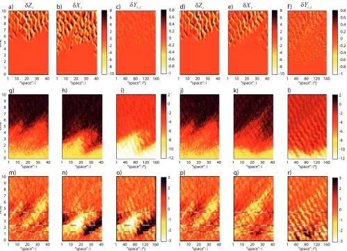
Fig. 3. Upper row: dynamics of a single realization of perturbations of the initial condition for (a, d) the simplified L96 model, and (b, c) the slow-fast variables,δxi andδyj,iof the L96 model with weak couplingh=0.3 and (e, f) with strong couplingh=1. The initial perturbations were randomly chosen according to a Gaussian distribution with standard deviationσ forδzandδx, and 0 forδy. Middle row: the same as in the upper row but in logarithmic scale. Lower row: the same as in the middle row but taking away the mean at each time. In order to ease their comparison, panels a, g, m are respectively identical to panels (d, j, p). Notice also the different scales in each case.
a given standard deviation σ, defined as a fraction of its stationary value, σ=10−4σst, withσst∼3.2. The
spatio-temporal evolution of the ensemble is characterized by the non-infinitesimal fluctuationsδzi(t )≡z0i(t )−zi(t )between
the perturbed member and the control trajectory. These fluc-tuations follow an equation that can be written separating lin-ear and non-linlin-ear terms as:
dδzi
dt =zi−1(δzi+1−δzi−2)
+δzi−1(zi+1−zi−2)−δzi+O
δz2
(3)
O(δz2)representing terms of second, or larger, order. When fluctuations are small, nonlinear terms can be neglected and the evolution can be considered as infinitesimal. As the growth is exponential, due to the multiplicative character of
the linear Eq. (3), in a short time the nonlinear terms be-come important and a new evolution emerges, which is not infinitesimal (finite fluctuations). Figure 3a shows an ex-ample of the growth of perturbations in one scale systems. This figure shows that, after some time (aroundt=5) with this exponential growth, the perturbations reach locally the amplitude of the system (the scale of the plot is the same as the corresponding panel in Fig. 2) and saturate. Be-fore that time, the spatio-temporal growth of errors follows a characteristic dynamics where temporal and spatial com-ponents interplay leading to characteristic localized growth patterns. In order to see these initial stages of the spatial evolution, Fig. 3g shows the same growth process, but in logarithmic scale, that is, we represent the log-perturbations hi=log|δzi|. In logarithmic scale the progressive growth
phenomenon graphically Fig. 3m shows the deviation of the log-perturbation to its spatial mean, hi−m1Phi. The
ini-tially Gaussian perturbations get quickly localized in a flow-dependent structure which is kept until saturation due to non-linear effects.
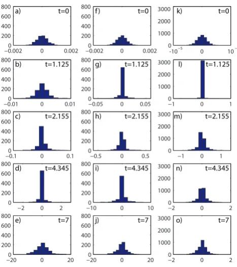
This behavior is represented in Fig. 4a–e, which shows the histograms of the perturbationsδzi(t )at five different times:
the initial (t=0) and saturated (t=7) times (with Gaussian-like distributions) and three intermediate stages indicated with dashed lines in Fig. 3m (with localized distributions). To get a higher statistical significance we used 20 random initial perturbations to build the histograms. The behavior shown is typical of the growth of a random initial perturba-tion in a spatio-temporal chaotic system with only one active scale. Initially the spatial distribution is Gaussian by con-struction (panel a). The further evolution shows a progres-sive localization (Fig. 4b, c, d) whose distributions exhibits a non-gaussian profile. This spatial localization is an effect of chaotic systems in their infinitesimal evolution (when per-turbations are in the tangent manifold). It is well known that initial perturbations in chaotic systems tend to their main Li-apunov vector (Baker and Gollub, 1996). Roughly speaking we can say that the initial random perturbation is going to the chaotic attractor adopting the form of the main Liapunov vec-tor. The localization process ends when either the Liapunov vector is reached or the amplitude is large enough to induce the appearance of nonlinear effects. As said above, when nonlinear terms are important a second regime appears where the localization gained is destroyed (Fig. 4e). (see Guti´errez et al., 2008, for more details).
3.2 The MVL approach
Spatially localized structures follow logarithmic statisti-cal distributions (log-normal, log-Poissonian,...) and thus they are better analyzed in their logarithmic representa-tion. Moreover, it is known that the logarithmic transforma-tion of infinitesimal perturbatransforma-tions behave as growing rough surfaces, which allows a precise analysis by using tech-niques borrowed from statistical physics (L´opez et al., 2004). The Mean-Variance Logarithmic (MVL) diagram (Guti´errez et al., 2008) was introduced with these premises in mind. The MVL diagram is based on the log-perturbations, defined as the logarithm of the absolute value of the perturbations de-fined above, i.e.,hi(t )=log|δzi(t )|. It is a two-dimensional
representation displaying in the abscissa the spatial average of the log-perturbations (the M-value):
M(t )= 1
m
X
i
hi(t ) (4)
and in the ordinate the spatial variance (the V-value):
V (t )= 1
m
X
i
(hi(t )−M(t ))2. (5)
0 0 200 400 600 800
−0.002 0.002
a) t=0
−0.0020 0 0.002 200
400 600 800
f ) t=0
0 0 1000 2000 3000
10−5 -10−5
k) t=0
−0.010 0 0.01
200 400 600 800
b) t=1.125
−0.10 0 0.1
200 400 600 800
c) t=2.155
−200 0 20
200 400 600 800
e) t=7
−2 0 2
0 200 400 600 800
d) t=4.345
−0.05 0 0.05
0 200 400 600 800
g) t=1.125
−0.5 0 0.5
0 200 400 600 800
h) t=2.155
−200 0 20
200 400 600 800
j) t=7
−100 0 10
200 400 600 800
i) t=4.345
−1 0 1
0 1000 2000
3000 l) t=1.125
−1 0 1
0 1000 2000
3000m) t=2.155
−2 0 2
0 1000 2000
3000 o) t=7
−2 0 2
0 1000 2000
3000 n) t=4.345
Fig. 4. Histograms of 20 perturbations of an initial condition for (a)–(e) the simplified L96 model, (f)–(j) the slow variablesxiof the L96 model with strong coupling (h=1), and (k)–(o) the fast variable
yj,iof the L96 model. For each column, the different rows from top to bottom represent the initial, three intermediate and the final times, corresponding to the horizontal lines depicted in Fig. 3.
The evolution (growth) of the initial perturbation is given by the parametric curve (M(t ),V (t )) in the diagram. It can be shown that the horizontal axis represents the spatially-averaged error growth in time (related to the leading Lia-punov exponentλasM(t )∼λt), whereas the vertical evo-lution represents the spatial dynamics given by a changing spatial correlation length (characteristic spatial scale) of the perturbation field. The resulting spatio-temporal growth is a combined effect of both interplaying components (Guti´errez et al., 2008), and its dynamics can be characterized with the MVL diagram.
0 2 4 6 8 10 −14
−12 −10 −8 −6 −4 −2 0 2
t
M(t)
0 2 4 6 8 10
1 1.5 2 2.5
t
V(t)
−141 −12 −10 −8 −6 −4 −2 0 2
1.5 2 2.5
M(t)
V(t)
1E−4 1E−6
Finite space barrier
Non-linear barrier
a) b)
c)
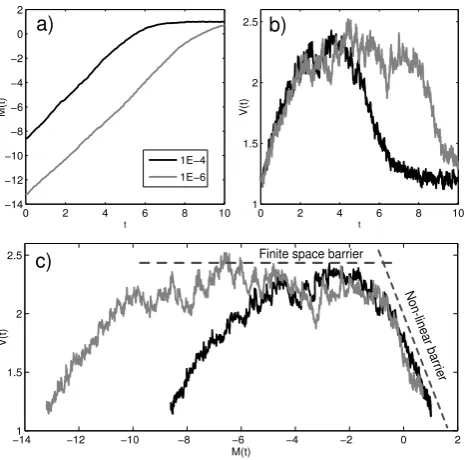
Fig. 5. (a) Temporal evolution of the M-component of the growth of perturbations of the example shown in Fig. 3a, (b) temporal evo-lution of the V-component, (c) MVL diagram. Two different values ofσfor the standard deviation of the initial perturbations have been considered.
of spatial structure, or localization, in the original represen-tation. In order to see the effect of the amplitude of the ini-tial perturbation, two different values ofσ were considered: 10−4(as in Fig. 3a) and 10−6. When the initial perturbation is small enough (the caseσ=10−6)V saturates due to the fi-nite size of the system, before the action of non-linear terms. In other words, the initial perturbation, that tends to the main Liapunov vector, reaches this limit in an infinitesimal evolu-tion before being perturbed by the non linear terms.
As we can see in this example, the MVL Diagram is a pow-erful tool to analyze the dynamics of initial perturbations. Its implementation and physical interpretation are very simple which increases their practical value: An increase (decrease) of variance (V-value) means an approach to (separation from) the tangent manifold of the chaotic attractor, which can be used as a quantifier of dynamic assimilation. Finally note that its use is not limited to the analysis of initial perturba-tions but, in general, it is valid for the analysis of any dynam-ical state as those appearing in data assimilation and synchro-nization (Szendro et al., 2009).
4 Growth of perturbations with multiple scales
The fluctuation dynamics with multiple scales is very depen-dent of the intensity of the coupling between both scales. In the case of weak coupling the fast and slow variables follow a similar dynamics of fluctuations: The saturation time of both variables is close (Fig. 3h and i), and the patterns of
lo-calization are also similar (Fig. 3n and o). This result is not surprising since, as seen in Sect. 2, the fast scale is deeply conditioned by the slow scale. The spatial and temporal vari-ations of their fluctuvari-ations are then similar.
The strong coupling case is completely different. The growth of perturbations follows a more complex pattern. Firstly, the saturation time of the fast variable is shorter than that of the corresponding slow variable (Fig. 3l and k). The fast variable saturates att=1, while the slow variable keeps a pattern similar to the simplified L96 case (Fig. 3l, k, and j). Secondly, the fast variable in the case of strong coupling shows a finer spatial resolution (Fig. 3l and r) than the corre-sponding ones in the weak coupling case (Fig. 3i and o). In fact, the characteristic pattern of traveling waves described before is more clearly observed in the case of strong cou-pling. Finally, the localization patterns shown by panels in the bottom row of Fig. 3 show a different spatial be-havior, since the saturation of the fast variables produces a cross-over in the slow ones with two separate regimes. Before the saturation of the fast variables, the growth of the slow ones follow the characteristic regime where per-turbations get progressively localized. This is better appre-ciated in the histograms (see Fig. 4f and g). When non-linear saturation effects appear in the fast variables (yield-ing the Gaussian-like spatial distribution of perturbations in Fig. 4m), the slow variables are also forced to lose the local-ized structure (Fig. 4h). Afterwards, when the fast variables are fully saturated (cross-over point), the slow ones recover the localized spatial structure (Fig. 4i) until they also satu-rate (Fig. 4j). These two characteristic regimes have not been reported elsewhere and are a fundamental knowledge to un-derstand the different dynamical behavior of perturbations in multi-scale spatio-temporal models, including weather mod-els; for instance, atmosphere-ocean coupled models show different time scales for the different components: fast at-mosphere and slow ocean.
4.1 MVL diagrams
-15 -10 -5 0 5
M(t)
1 1.5 2 3 4 5
2.5 3.5 4.5 5.5
V(t)
Zi Xi Yj ,i c)
1 3 5 8
0 2 4 6 7 9 10
t
1 1.5 2 3 4 5
2.5 3.5 4.5 5.5
V(t)
f)
1 3 5 8
0 2 4 6 7 9 10
t
1 1.5 2 3 4 5
2.5 3.5 4.5 5.5
V(t)
b)
1 3 5 8
0 2 4 6 7 9 10
t
1 1.5 2 3 4 5
2.5 3.5 4.5 5.5
V(t)
i)
1 3 5 8
0 2 4 6 7 9 10
t
-14 -12 -10 -6 -2
-8 -4 0 2
M(t)
e)
1 3 5 8
0 2 4 6 7 9 10
t
-14 -12 -10 -6 -2
-8 -4 0 2
M(t)
a)
1 3 5 8
0 2 4 6 7 9 10
t
-14 -12 -10 -6 -2
-8 -4 0 2
M(t)
h)
Zi Xi Yj ,i g)
1 1.5 2 3 4 5
2.5 3.5 4.5 5.5
V(t)
-15 -10 -5 0 5
M(t)
j) Zi
Xi Yj ,i
1 1.5 2 3 4 5
2.5 3.5 4.5 5.5
V(t)
-15 -10 -5 0 5
M(t)
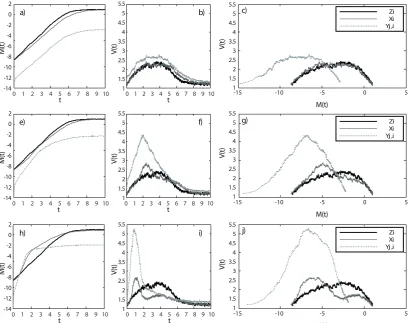
Fig. 6. Time series of the mean (a, e, h) and variance (b, f, i) of the log-perturbations of a simplified L96 model (black) and the slow (xi, dark gray) and fast (yj,i, light gray) components of a two-scale L96 model. (c, g, j) MVL diagrams corresponding to the previous components. The upper row (a, b, c) is for weak couplingh=0.26, the medium row (e, f, g) is for medium couplingh=0.6 and the lower row is for strong couplingh=1. All curves are averages of 200 realizations (see text).
a greater slope in the logarithmic amplitude (Fig. 6h) than in the weak coupling configuration. There is a second regime, after the saturation of the fast variable, where the dynamics of the slow variables becomes independent and the slope of the logarithmic amplitude is smaller. In terms of the variance (Fig. 6b, f, and i) there are two effects on the fast variable when increasing the coupling parameter. The first is the ear-lier decay of the variance with the increasing coupling. This is related to the fast arrival to the non-linear barrier caused by the faster growth of the amplitude. The second effect is that increased coupling leads to a larger maximum variance (i.e. localization of the perturbation) reached by the fast variable. That is, the stronger the coupling, the more relevant the fast variable becomes and, thus, the finer the spatial detail it can develop.
It is worth remarking the complex patterns of the slow variable in this case. Four regimes are observed in the MVL diagram (Fig. 6j). The first two are induced by the beha-vior of the fast variables. After the saturation of this vari-able the slow one continues increasing the structure until its
own saturation. In Fig. 6h and i, it is apparent that when the amplitude of the fast variable is saturated (aroundt=2), the variance continues its evolution in a slowing down pro-cess that lasts until the saturation time of the slow variable (aroundt=7−8).
0 0.1 0.2 0.3 0.4 0.5 0.6 0.7 0.8 0.9 1 2
2. 5 3 3. 5 4 4. 5 5 5. 5
max(
V
)
Coupling (h)
Weak Medium Strong
Fig. 7. Maximum value of the variance of the log-perturbations of the fast componentsyj,iof the two-scale L96 model (Vcomponent of the MVL-diagram) as a function of the coupling parameterh.
4.2 Fast dynamics and effective noise
It is interesting to investigate the role played by the fast vari-ables in the dynamics of a multi-scale system. The possibility of parametrization of fast degrees of freedom by an equiva-lent noise is important to reduce the complexity of a problem (Just et al., 2001). For the sake of illustration we explore this possibility in our case.
In a case with weak coupling, where the slow variable is dominant, the fast variables play a secondary role and they could be substituted by a weak additive noise without altering the main dynamics. However, when the coupling is strong, the existence of two distinct regimes impede the existence of an equivalent effective noise, even to reproduce the second regime, when fast variables are saturated and the slow ones become dominant. We show in Fig. 8 the effect of adding a random Gaussian noise in a one-scale model with an inten-sity equivalent to those of the fast source term (i.e. with the same mean and standard deviation). The noise is added at the saturation time but we checked that the effect is similar when it is placed in any other previous time. We can see that the equivalent noise does not reproduce the dynamics of the two-scale model. The added noise is not dynamically assim-ilated,V decreases until the noise is assimilated, and a very different pattern is observed in the MVL diagram (Fig. 8). Note that starting in a previous time is not a solution since at these times the fast variable is dominant and cannot be sub-stituted by a passive component. How to find a dynamically compatible noise to reduce the two-scale model in this case is a difficult problem that exceeds the scope of this paper. Figure 8 is a good illustration of this problem. Note that this may have important implications in order to define appropri-ate initial perturbations for ensemble prediction in coupled atmosphere-ocean models.
Zi
Xi* Xi Yj ,i
1 1.5 2 3 4 5
2.5 3.5 4.5 5.5
V(t)
1 1.5 2 3 4 5
2.5 3.5 4.5 5.5
V(t)
-14 -12 -10 -6 -2
-8 -4 0 2
M(t)
3 7
1 2 5 6 8 9 10
0 4
t
3 7
1 2 5 6 8 9 10
0 4
t
-14 -10 M(t) 5 0 2
a) b)
c)
Fig. 8. Growth of perturbations in the two-scale model (xi;yj,i) with strong coupling (h=1) versus the single-scale model (zi) and the single-scale model with an equivalent noise (xi∗): (a) temporal evolution of the M-component of the growth of perturbations, (b) temporal evolution of the V-component, (c) MVL diagram.
5 Conclusions
The spatio-temporal dynamics of the error growth in the two-scale model proposed by Lorenz (1996) has been character-ized by means of the MVL diagram. For comparison pur-poses, a simplified version of the model with a single scale was also considered. This latter model was already charac-terized by Guti´errez et al. (2008) and evolves from a small random initial perturbation by increasing the mean error and the localization until the finite-size and non-linear effects be-come large and destroy the localization gained reaching a sta-tionary state.
Finally, we tried to reproduce the second hump experi-enced by the slow variables in the MVL diagram by sub-stituting the fast variables (once saturated) by an equivalent noise term in the governing equation for the slow variables, but our attempt was unsuccessful.
This complex behavior may be relevant for other systems such as the atmosphere-ocean system where there are fast varying variables (in the atmosphere) gaining and losing the structure much faster than others (in the ocean, for instance). This issue could be made evident by analyzing atmosphere-ocean coupled model output from existing ensemble predic-tion systems. Of course, this is out of the scope of the present work and will be dealt with in a forthcoming paper.
Acknowledgements. The authors are grateful to the Comisi´on
Interministerial de Ciencia y Tecnolog´ıa (CICYT, CGL2004-02652 and CGL2005-06966-C07-02/CLI grants) for partial support of this work.
Edited by: O. Talagrand
Reviewed by: three anonymous referees
References
Baker, G. and Gollub, J.: Chaotic dynamics: an introduction, Cam-bridge University Press, UK, 1996.
Fern´andez, J., Primo, C., Cofino, A. S., Rodr´ıguez, M. A., and Guti´errez, J. M.: MVL Spatiotemporal analysis for model inter-comparison in EPS. Application to the DEMETER multi-model ensemble, Clim. Dynam., 33, 233–243, 2008.
Guti´errez, J. M., Primo, C., Rodr´ıguez, M. A., and Fern´andez, J.: Spatiotemporal characterization of Ensemble Prediction Sys-tems – the Mean-Variance of Logarithms (MVL) diagram, Non-lin. Processes Geophys., 15, 109–114, doi:10.5194/npg-15-109-2008, 2008.
Just, W., Kantz, H., Rodenbeck, C., and Helm, M.: Stochastic mod-elling: replacing fast degrees of freedom by noise, J. Phys. A, 34, 3199–3213, 2001.
L´opez, J. M., Primo, C., Rodr´ıguez, M. A., and Szendro, I.: Scaling properties of growing noninfinitesimal pertur-bations in space-time chaos, Phys. Rev. E, 70, 056224, doi:10.1103/PhysRevE.70.056224, 2004.
Lorenz, E. N.: Predictability-a problem partly solved, in: Pro-ceedings of ECMWF seminar Predictability, ECMWF Seminar Proceedings, ECMWF, Reading, UK, Seminar on Predictability, Vol. I, 1–19, 1996.
Lorenz, E. N. and Emanuel, K.: Optimal sites for supplementary weather observations: Simulation with a small model, J. Atmos. Sci., 55, 399–414, 1998.
Orrell, D.: Model Error and Predictability over Different Timescales in the Lorenz96 systems, J. Atmos. Sci., 60, p. 2219, 2003.
Primo, C., Szendro, I., Rodr´ıguez, M. A., and Guti´errez, J. M.: Er-ror growth analysis in systems with spatial chaos: Coupled map lattices and global weather models, Phys. Rev. Lett., 98, 108501, doi:10.1103/PhysRevLett.98.108501, 2007.
Szendro, I., Rodr´ıguez, M. A., and L´opez, J.: On the problem of data assimilation by means of synchronization, J. Geophys. Res., 114, D20109, doi:10.1029/2009JD012411, 2009.