www.nonlin-processes-geophys.net/16/381/2009/ © Author(s) 2009. This work is distributed under the Creative Commons Attribution 3.0 License.
Nonlinear Processes
in Geophysics
The interaction of free Rossby waves with semi-transparent
equatorial waveguide – wave-mean flow interaction
G. M. Reznik1,2and V. Zeitlin1
1Laboratory of Dynamical Meterology, Ecole Normale Superieure and University Paris 6, 24, rue Lhomond, 75005, Paris, France
2now at: P.P. Shirshov Institute of Oceanology, 36 Nakhimovsky av., 117997, Moscow, Russia
Received: 21 October 2008 – Revised: 19 February 2009 – Accepted: 14 April 2009 – Published: 7 May 2009
Abstract. Nonlinear interactions of the barotropic Rossby
waves propagating across the equator with trapped baroclinic Rossby or Yanai modes and mean zonal flow are studied within the two-layer model of the atmosphere, or the ocean. It is shown that the equatorial waveguide with a mean cur-rent acts as a resonator and responds to barotropic waves with certain wavenumbers by making the trapped baroclinic modes grow. At the same time the equatorial waveguide pro-duces the barotropic response which, via nonlinear interac-tion with the mean equatorial current and with the trapped waves, leads to the saturation of the growing modes. The ex-cited baroclinic waves can reach significant amplitudes de-pending on the magnitude of the mean current. In the ab-sence of spatial modulation the nonlinear saturation of thus excited waves is described by forced Landau-type equation with one or two attracting equilibrium solutions. In the lat-ter case the spatial modulation of the baroclinic waves is expected to lead to the formation of characteristic domain-wall defects. The evolution of the envelopes of the trapped Rossby waves is governed by driven Ginzburg-Landau equa-tion, while the envelopes of the Yanai waves obey the “first-order” forced Ginzburg-Landau equation. The envelopes of short baroclinic Rossby waves obey the damped-driven non-linear Schrodinger equation well studied in the literature.
1 Introduction
The present paper is the second part of the geophysical fluid dynamics investigation of nonlinear phenomena due to res-onant interaction of free modes and modes trapped in the equatorial waveguide. In the first part (Reznik and Zeitlin, 2007) we have studied nonlinear interactions of a free wave
Correspondence to: V. Zeitlin ([email protected])
and a pair of trapped modes in the framework of the simplest two-layer equatorial beta-plane model with a rigid lid. Let us remind that free modes in the model are barotropic Rossby waves, while all baroclinic modes (Kelvin, Inertia-Gravity, Rossby and Yanai ones) are trapped. We showed in Part 1 that although in the linear approximation the barotropic Rossby wave does not “feel” the equator and propagates freely across the equatorial waveguide, this wave resonantly excites the waveguide Rossby or Yanai modes if nonlinear effects are taken into account. The amplitudes of the excited modes first grow exponentially in time, and then stabilize at the level greatly exceeding the amplitude of the incoming free wave. The envelope of the trapped waves obeys the so-called resonantly excited Ginzburg-Landau (GL) equation, or a pair of coupled GL-equations, which describes the forma-tion of specific spatio-temporal patterns. In turn, nonlinear interactions of the waveguide modes engender a secondary barotropic wave which propagates out of equator toward the poles, grows in time and becomes comparable with the pri-mary free wave.
trapped mode greatly exceeds the free wave amplitude, but the mechanisms of generation and saturation are essentially different. The study of these mechanisms is the main goal of the present paper. Preliminary results were presented in Reznik and Zeitlin (2007b), where some illustrations may be also found.
The paper is organized as follows: in Sect. 2 we de-scribe the two-layer shallow water model on the equatorial beta-plane, remind the spectrum of its linear excitations and derive the synchronism contitions for resonant interaction barotropic wave – trapped wave – mean zonal flow. In Sect. 3 we describe the resonant excitation of the trapped modes fol-lowing from the straightforward asymptotic analysis in non-linearity parameter. In Sect. 4 we rearrange the asymptotic expansions in order to take into account the eventual nonlin-ear saturation of the growing modes, and show that such satu-ration indeed takes place. We derive the equations describing the effects of spatial modulation in Sect. 5, and conclude in Sect. 6.
In order that technical details do not overshadow the main message, we limit ourselves in the main body of the paper by the mathematically simplest case of the layers of equal depth, and purely baroclinic zonal flow. The general case is discussed in Appendix A. By the same reason all cumber-some calculations/formulae are relegated to Appendices B, C.
2 The model, its linear wave spectrum and the
synchronism conditions
2.1 The equations of the model and the linear wave spectrum
The simplest model taking into account the phenomena we are interested in is the 2-layer equatorial rotating shallow wa-ter model with the rigid lid and flat bottom boundary condi-tions which was already used in Reznik and Zeitlin (2007). The equations of the model may be conveniently rewritten in terms of the barotropic streamfunctionψ, baroclinic veloc-ity u=(u, v), and the thickness deviationhof the upper layer with respect to its mean value (Reznik and Zeitlin, 2007; Be-nilov and Reznik, 1996):
∇2ψt+ψx= h
−J (ψ,∇2ψ )−s(∂xx−∂yy)[(1+rh)(uv)] +s∂xy
h
(1+rh)(u2−v2)ii (1)
ut+∇h+yzˆ×u=−J (ψ,u)+u·∇(zˆ×∇ψ )−ru·∇u+s
(2hu·∇u+u u·∇h)], (2)
ht+∇·u= h
−J (ψ, h)−r∇·(uh)+s∇·
h2ui, (3) where here and below the subscripts are used for the cor-responding partial derivatives, andJ denotes the Jacobian.
The Eqs. (1–3) are written in non-dimensional form using the standard equatorial shallow-water dynamics scaling:
L=(g
0H
s)1/4 √
β ;T=
1
βL; U= g01H
βL2 . (4)
The values of the parameters s andr (which was called q
in Part 1, we reserve the notationq for other purposes, see below) depend on the details of stratification (the standard derivation is based on layer averaging of the primitive equa-tions with flat bottom and rigid lid boundary condiequa-tions, cf. e.g. Zeitlin, 2007):
r=H−2H1
H , s=
Hs H, =
1H Hs
, (5)
where 1H denotes a typical variation of the interface,
Hs=H1(HH−H1), and the nonlinearity parameteris assumed to be small1. In the Eqs. (4), (5)H1, H2=H−H1 are the the upper and lower layer thicknesses, g0 is the stan-dard reduced gravity parameter,Lis the baroclinic equatorial Rossby radius.
The rigid lid boundary condition, often used in studies of equatorial dynamics (cf. e.g. Majda and Biello, 2003 and ref-erences therein), is well adapted to the problem of free-wave – trapped wave interactions we address, as it allows for free propagation of the equatorial beta-plane barotropic waves (see below). If it is relaxed, the barotropic waves would be also meridionally confined (although with a larger char-acteristic decay length, than for the baroclinic waves). We should note, however, that the barotropic Rossby waves in the shallow-water model on the sphere are not trapped in the vicinity of the equator (e.g. Longuet-Higgins, 1968; Muller, 2000a); it is also known from observations that extratropical waves do arrive towards tropics, e.g. Hamilton et al. (2004).
The linear spectrum of the model consists of plane barotropic Rossby waves which may propagate at any angle with respect to the equator:
˜
ψ0=Aψei(θ+ly)+c.c.; θ=kx−σ t, (6) and have the dispersion relation:
σ=−k/(k2+l2), (7)
and the trapped baroclinic equatorial waves
(u,˜ v,˜ h)˜ =(iUm, Vm, iHm) Aeiθm+c.c.; θm=kx−σmt (8) with the dispersion relation
amplitudesUm, Vm=φm, Hm decay rapidly away from the equator (y=0):
φm(y)=
Hm(y)e−
y2
2
p
2mm!√π, Um(y)=
σmyφm−kφm0 σm2−k2 , Hm(y)=
kyφm−σmφm0 σ2
m−k2
, (10)
whereHm(y)are the Hermite polynomials and the prime meansy-differentiation. Equator, thus, is a wave-guide trans-parent for some type of waves in the linear approximation.
One can readily see that any equatorial zonal current
u= ¯u(y), h= ¯h(y), v=0, yu¯+ ¯hy=0, ψ= ¯ψ (y) (11) is an exact solution to (1–3). In the main body of the paper we will present the calculations in the technically simplest case when the zonal flow is purely baroclinic and the upper and lower layers are of the same depth:
¯
ψ (y), r=0. (12)
The discussion of the general case, which is technically much more involved, but not different in essence, is relegated to Appendix A.
In order to measure the strength of the zonal flow we in-troduce a parameterα:
u=αu(y), h¯ =αh(y), y¯ u¯+ ¯hy=0. (13) In what follows it is assumed that the zonal flow is suffi-ciently strong, so thatαis negative, but at the same time it is sufficiently weak and does not alter the structure of the wave modes in the lowest order. This assumptions means that
−1<α≤0, (14)
so that nonlinear terms in (1–3) remain small. In addition, we will suppose that the mean flow rapidly decreases out of the equator.
2.2 The synchronism conditions
We will analyze the nonlinear interaction of the barotropic wave (6) with the zonal flow (13). As is easy to see from (1–3), the m-th baroclinic trapped mode is resonantly ex-cited by such interaction if its zonal wavenumberk and the frequencyσ coincide with the corresponding wavenumber and frequency of the barotropic mode. As follows from (7), (9) this is possible if the meridional wavenumber of the barotropic wave obeys the equation:
l2=2m+1−σm2>0, m=0,1, .... (15) The dispersion relation for the trapped Yanai wave,m=0 has the form:
σ0=k/2+ q
1+k2/4, (16)
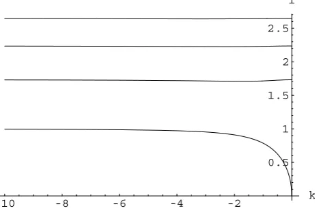
-10 -8 -6 -4 -2 k
0.5 1 1.5 2 2.5 l
Fig. 1. Solutions to the synchronism conditions in the phase-space
k−lof the barotropic wave for meridional modes withm=0, 1, 2, 3.
therefore (15) is satisfied at any k<0. For trapped Rossby waves,m≥1, (15) is also always satisfied because with high accuracy (Boyd, 1983)
σm' − k
k2+2m+1, (17)
and
l2'2m+1− k
2
(k2+2m+1)2≈2m+1. (18) The relation (15) defines a curve in the(k, l)plane and thus, unlike the synchronism conditions in the triad case (Reznik and Zeitlin, 2007), only a discrete spectrum of barotropic Rossby waves will resonate with equatorial waveguide modes in the presence of the equatorial current, cf. Fig. 1
3 Resonant excitation of the trapped modes
3.1 General approach and removal of resonances
The standard method for treating the resonant excitation of waves consists in applying multiple time-scale asymptotic expansions in small parameter ( in the present case) to the initial wave configuration, to be completed by multiple space-scales if the effects of spatial modulation are to be treated. Each approximation is described by the forced lin-earized Eqs. (1–3):
∇2ψt+ψx=Qψ (19)
asymptotic expansions self-consistent, and leads to determi-nation of the (slow-)time-dependence of the wave amplitude, eventually exhibiting growth. The asymptotic analysis which will be used below involves, as usual, the removal of secular terms arising in the r.h.s. of the Eqs. (19–20). The solution is bounded provided the following orthogonality conditions are satisfied:
h ˆψ Qψix,y,t=0, (21)
Z ∞ −∞
dyh ˆuQu+ ˆvQv+ ˆhQhix,t=0, (22)
whereψ ,ˆ u,ˆ v,ˆ hˆ is an arbitrary bounded solution of the
ho-mogeneous Eqs. (19), (20), respectively, and the angle brack-ets denote the averaging defined in a usual way:
h...ix= lim Lx→∞
1 2Lx
Z Lx
−Lx
dx ..., (23)
and analogously for other variables. In what follows, the source terms are of the form:
Qψ,...,h= X
q
Qqψ,...,h(y)ei(kqx−σqt ), (24)
withQqψ,...,h(y)rapidly decaying aty→±∞. One can read-ily show that for such Qψ,...,h the conditions (21), (22) are not only necessary, but also sufficient for existence of bounded solutions to (19), (20) ifkq6=0, σq6=0. Applying these conditions allows to determine the slow-time depen-dence of the wave-amplitudes.
Another important ingredient of the method is the use of asymptotic expansions including inverse powers of the small parameter to study eventual nonlinear saturation (cf. e.g. Minzoni and Whitham, 1977), once the resonant growth is confirmed by straightforward expansions.
In the rest of the present section below we will establish the fact of resonance growth of the trapped waves due to the free wave-mean-trapped wave interaction. The nonlinear sat-uration will be studied in Sect. 4 on the basis of rearranged asymptotic expansions.
3.2 Governing equations for interacting waves and zonal flows
Following the standard asymptotic approach, the solution of the Eqs. (1–3) is sought in the following form:
(ψ, u, v, h)=(ψ(0), u(0), v(0), h(0))(x, y, t, T )+
(ψ(1), u(1), v(1), h(1))(x, y, t, T )+..., (25) whereT=tis the slow time. Here the quantities with the su-perscript(0)satisfy the linearized version of (1–3) and com-prise the barotropic Rossby wave:
ψ(0)=Aψei(θ+ly)+c.c., (26)
and the baroclinic field, which consists of the trapped baro-clinic wave (8) on the background of the zonal barobaro-clinic current (13):
u(0), v(0), h(0)=u¯(0),0,h¯(0)(y, T ) +
˜
u(0),v˜(0),h˜(0)
(x, y, t, T ) (27)
˜
u(0),v˜(0),h˜(0)(x, y, t, T )=a−1
2(iU, V , iH ) A(T )eiθ+c.c.,
a= Z +∞
−∞
dy (U2+φ2+H2). (28)
With this normalization the energy density of the trapped mode is always equal toA2.
Obviously, the baroclinic mode (28) and the barotropic wave (26) are in resonance. The equations for the correc-tions(ψ(1), u(1), v(1), h(1))are (for simplicity, we put the ex-ponentαin (13) to be zero in the rest of this section):
∇2ψt(1)+ψx(1)=Nψ, (29) u(t1)−yv(1)+h(x1)=− ¯u(T0)− ˜u(T0)+Nu, (30) vt(1)+yu(1)+hy(1)=− ˜vT(0)+Nv, (31) ht(1)+ux(1)+v(y1)=− ¯h(T0)− ˜h(T0)+Nh, (32) where the nonlinear interaction terms are given by (cf. 1–3):
Nψ=−J (ψ(0),∇2ψ(0))− 1 4[(∂xx
−∂yy) (u(0)v(0))−∂xy(u(0) 2
−v(0)2) i
, (33)
Nu=−J (ψ(0), u(0))+u(0)·∇ψy(0), (34) Nv=−J (ψ(0), v(0))−u(0)·∇ψx(0), (35)
Nh=−J (ψ(0), h(0)). (36)
3.3 Slow evolution
It is easy to see (cf. also Reznik and Zeitlin, 2007) that the expressionNψ does not contain resonant terms due to the fast decay iny of the functionsU (y), φ (y), H (y). By this reason the amplitude of the barotropic wave does not depend on slow time in this approximation.
The equations determining corrections to the baroclinic component of the zonal flow are obtained by averaging the Eqs. (30–32) inx:
¯
u(t1)−yv¯(1)=− ¯u(T0)− ¯Ru, (37) ¯
vt(1)+yu¯(1)+ ¯h(y1)=− ¯Rv, (38) ¯
h(t1)+ ¯vy(1)=− ¯h(T0)− ¯Rh, (39) where
¯ Ru=
l2φ+kU0AψA∗eily+c.c., ¯
Rv=ik φ0+2ilφ+kUAψA∗eily+c.c., ¯
Rh=
kH eily
0
From the dispersion relation (9) and Eqs. (10), (15) we obtain the following relation
l2φ+kU0=−kyH, (41)
which allows to rewriteR¯u,R¯has ¯
Ru=−yD, R¯h=Dy, D=−kAψA∗H eily+c.c.. (42) By using the substitution v¯(1)→ ¯v(1)+D it is easy to show that bounded solutions of (37–39) exist if
¯
u(T0)= ¯h(T0)=0, (43)
and thus the baroclinic zonal flow in the first approximation does not depend on slow time either.
A group of resonant terms in the r.h.s. of (30–32) is due to the lowest-order trapped wave (28). To re-move the resonances, we use the condition (22) with
(u,ˆ v,ˆ h)ˆ =(−iU, φ,−iH )e−iθ; as a result we obtain the fol-lowing evolution equation for the amplitudeA:
AT=−kLψAψ, (44)
where
Lψ= 1 √
a
Z +∞ −∞
dy eilyh(u(0)U )0+U u(0)0+H h(0)0−kφu(0)i. (45) As follows from the previous analysis, the r.h.s. of (44) does not depend on the slow timeT, i.e. the amplitude of the baro-clinic wave A grows in absolute value with increasing T. Thus, the interaction of the free barotropic Rossby wave with zonal flow results in effective generation of a trapped baro-clinic mode. An important distinction from the case of triad interactions (Reznik and Zeitlin, 2007) is linear, and not ex-ponential, growth in time. We show in Appendix A that this conclusion is also valid for nonzerorandψ¯.
Thus, we come to an important conclusion that for any zonal current there exist infinitely many barotropic Rossby waves which, by interacting with the current, generate grow-ing in time trapped baroclinic modes. This growth is linear, and not exponential, unlike the triad case (Reznik and Zeitlin, 2007). As will be shown below, the saturation mechanism is also different.
4 Nonlinear saturation of the growing baroclinic modes: modified asymptotic expansions in
4.1 The lowest-order approximation
The growth of the trapped baroclinic mode means that the en-ergy of the system: barotropic wave + zonal flow + trapped mode is not conserved. As in the triad case (Reznik and
Zeitlin, 2007), the energy balance following from the lowest-order equations (linearized 1–3) and the first-lowest-order Eqs. (29– 32)
E0=
s
2 Z ∞
−∞
dyhu(0)2+v(0)2+h(0)2ix
+ Z ∞
−∞
dy h∇ψ(0)·∇ψ(1)ix=const, (46) means that the growing energy of the trapped mode is com-pensated by the interaction energy of the primary barotropic fieldψ(0)and the correction to this fielsψ(1) arising due to the self-interaction of the baroclinic wave. This correction, which will be called below the secondary barotropic wave, is found from the Eq. (29):
∇2ψt(1)+ψx(1)=− 4 h
(∂xx−∂yy)(u(0)v(0))−∂xy(u(0)2−v(0)2)i. (47) It is clear that ψ(1) should also grow with slow time. The interaction ofψ(1)with the zonal flow and with the baroclinic wave arrests the growth of the amplitudeA, as in the triad case in Reznik and Zeitlin (2007).
The saturation process appears to be rather sensitive to the strength of the baroclinic zonal flow, i.e. to the value of the parameterα in (13). Therefore, we will not fixα, assum-ing only that it obeys (14). The situation here is more com-plicated than in Reznik and Zeitlin (2007), as the form of the asymptotic expansions should be adapted to the relative strength of the zonal flow, and various regimes are possible depending on the value ofα. Strictly speaking, the value of
αshould be first fixed, and only then the procedure of the asymptotic expansions be applied. We would like, however, to pursue our analysis as far as possible without loss of gener-ality, and therefore apply below an heuristic semi-qualitative approach by finding (approximate) solutions without fixing the value ofα. The results obtained in this way and displayed below were checked and confirmed by rigorous expansions for several typical sets of parameters.
Let us represent a solution of Eqs. (1–3) in the form:
(ψ, u, v, h)=(ψ(0), u(0), v(0), h(0))+(ψ(1), u(1), v(1), h(1)). (48) The lowest-order fields are written as follows:
ψ(0)=Aψei(θ+ly)+c.c.+ψ(1)(x, y, t, Tβ1, ), (49)
u(0), v(0), h(0)=αu¯(0),0,h¯(0)(y, Tα1)+β
˜
become, in principle, of the same order of magnitude as the primary barotropic wave. Therefore, it should be taken into account already in the lowest order, which is written in (49). Substitution of (50) into (47) shows thatψ(1)should have the form:
ψ(1)=1+α+βAψ(zw)+1+2βA2ψ(ww)+c.c., (51) where the first term in the r.h.s. arises from the interaction of the trapped mode with the zonal flow, and the second one from the self-interaction of the trapped wave. The functions
ψ(zw)andψ(ww)are calculated in Appendix B; the resulting solutionψ(1) obeying the radiation boundary conditions at
y→±∞has the form:
ψ(1)=1+α+βAψˆf(1)(y)eiθ+1+2βA2ψˆf(2)(y)ei2θ+c.c..(52)
4.2 The first-order corrections
Thus, the solution of the problem has the form (48), where the lowest-order approximation is given by (49), (50) while the first-order corrections are supposed to be small. The equations for the first-order corrections u(1), v(1), h(1) are written as follows:
ut(1)−yv(1)+hx(1)=−α+α1u¯(T0) α1−
β+β1u˜(0) Tβ1+N
(1)
u , (53) vt(1)+yu(1)+h(y1)=−β+β1v˜T(0)+Nv(1), (54)
ht(1)+u(x1)+vy(1)=−α+α1h¯(0) Tα1
−β+β1h˜(0) Tβ1
+Nh(1), (55) and the nonlinear termsNu(1), Nv(1), Nh(1)have the form: Nu(1)=Nu+
4 h
2h(0)u(0)ux(0)+v(0)u(y0) +u(0)
u(0)h(x0)+v(0)h(y0) i
, (56)
Nv(1)=Nv+
4 h
2h(0)
u(0)vx(0)+v(0)vy(0)
+v(0)u(0)hx(0)+v(0)h(y0)i, (57)
Nh(1)=Nh+
4
h(0)2u(0)
x +
h(0)2v(0)
y
. (58)
By applying averaging overx to the Eqs. (53–55) we get the equations for the zonal flow of the form (37–39) where
¯
Ru,R¯v,R¯h are replaced by hNu(1)ix, hNv(1)ix, hNh(1)ix, andu(T0), h(T0)– byα+α1u¯(T0)
α1,
α+α1h¯(0)
Tα1, respectively.
By using (34–36), (56–58), (49), (52), and (41) we find:
hNu(1)ix=−yD1, hNh(1)ix=D1y, (59)
where
D1=−βkAψA∗H eily−1+α+2β|A|2kHψˆf(1)+c.c., (60) cf. (42). As for the analogous system (37–39), the Eq. (59) mean that the termshNu(1)ix,hNh(1)ixin the r.h.s. of the equa-tions for the correcequa-tions to the zonal flow do not contain res-onances, i.e. we again come to the conclusion that the mean flow does not depend on time.
Another group of resonant terms in the r.h.s. of (53–55) is related to the wave proportional toeiθ. Eliminating these resonances gives the following evolution equation for the am-plitudeA:
β1A Tβ1+
2+2αpA+2+2βq|A|2A=−1+α−βkL
ψAψ. (61) HereLψ is given by (45), andp andq are constant com-plex coefficients which depend on the parameters of the in-teracting waves and of the zonal flow. Their expressions are given in Appendix C. Two important points are to be stressed: 1) Re p>0, and Re q≥0 which insures the saturation of the trapped baroclinic wave; 2)Re q=0,ifl2−3k2<0, and
Re q 6= 0,ifl2−3k2>0, which gives different properties of saturated solutions depending on the angle of incidence of the incoming barotropic wave.
4.3 Analysis of particular cases
As may be seen from (61) the growth of the trapped baro-clinic mode is provided by the constant forcing in the r.h.s. of the equation, which arises due to the interaction of the barotropic wave with the mean zonal current. The second and the third terms in the l.h.s. of (61) lead to saturation of the baroclinic amplitude becauseRe p, Re q≥0. The linear inAsecond term arises as a result of the interaction of the secondary barotropic modeψ(1) with the zonal flow, while the cubic inAthird term is a result of the interaction ofψ(1)
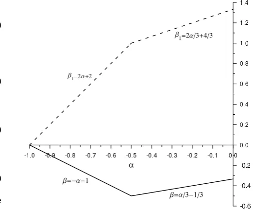
with the trapped baroclinic mode. The exponent α which defines the intensity of the zonal flow is fixed. The parame-tersβandβ1specifying the order of magnitude of the satu-rated baroclinic mode, and the slow time scale, respectively, are determined from the balance of pumping and damping in (61). Let us consider particular cases:
1. Let cubic saturation be dominant, i.e.
1+α−β=2+2β≤2+2α. (62)
As follows from (62)
β=1
3(α−1), α≥β≥− 1
2. (63)
2. Let linear saturation be dominant, i.e.
1+α−β=2+2α≤2+2β. (64)
Then
β=−(α+1), β≥−1
2≥α. (65)
On the basis of (63), (65) we come to the conclusion that at
α<−1
2 the linear saturation dominates, while atα>− 1 2 it is the cubic one. In both casesβ≥−1
2, i.e. the maximal attain-able baroclinic amplitude is of the order−12; such amplitude is reached at
α=β=−1
The slow time-scale is defined by the relation
β1=1+α−β. (67)
The dependence ofβ, β1onαis depicted in Fig. 2 Atα<−1
2the Eq. (61) may be rewritten as
ATβ1+pA=−kLψAψ; (68)
atα>−1
2, as
ATβ1+q|A|
2A=−kL
ψAψ; (69)
and, finally, atα=−1
2as
ATβ1+pA+q|A|
2A=−kL
ψAψ. (70)
While deriving (61), and hence (68–70), we did not use systematic asymptotic expansions, unlike what was done in Reznik and Zeitlin (2007). We rather used a semi-qualitative approach based on the physical considerations of balance of different contributions. To check the validity of the resulting evolution equations we applied the standard asymptotic pro-cedure for several typical values of the parameterαand con-firmed that in all of these cases the resulting equation for the baroclinic amplitude coincides with the corresponding equa-tion among (68–70). For instance, atα=0 (moderate mean zonal flow) we getβ=−1
3, β1= 4
3, i.e. the asymptotic expan-sion in powers of 13 should be applied. The correspond-ing amplitude equation has the form (69). Atα=−12 (strong mean zonal flow) we getβ=−1
2, β1=1, i.e. the asymptotic expansion in powers of12 should be applied and gives (70). Finally, atα=−2
3 (even stronger mean zonal flow) we get
β=−1
3, β1= 2
3, i.e. the asymptotic expansion should be again in powers of13 and results in (68). The limiting amplitude has the same order of magnitude as atα=0, but saturation is faster.
In what follows we will limit ourselves by the most general caseα=−1
2.
4.4 Analysis of the saturation process
By renormalization ofAandT
Tβ1→T=|p|Tβ1, A→ s
|q| |p|e
iArg(kLψAψ)A, (71)
the number of relevant parameters in (70) may be reduced:
AT+eiξA+eiη|A|2A=c, (72) where
ξ=Arg p, η=Arg q, c=|q|12|p|−32 kLψAψ. (73)
Fig. 2. Dependence of the exponents of the slow timeβ1, and of the saturation levelβon the exponentαdefining the intensity of the zonal flow.
Let us consider stationary solutionsA¯of (72). The following relations hold for the modulus and the argument ofA¯: cosξA¯
+cosη
A¯
3
=ccosArg(A),¯
sinξA¯ +sinη
A¯
3
=−csinArg(A),¯ (74) whence a cubic equation for the square modulus ofA¯readily follows:
| ¯A|6+2 cosχ| ¯A|4+| ¯A|2−c2=0, χ=ξ−η. (75) Applying Viet’s theorem it is easy to show that (75) has either three positive roots, or a single positive root. An elementary analysis shows that necessary and sufficient conditions of the existence of three roots are:
cosχ <− √
3
2 , F (x+)<c 2<F (x
−), (76)
where
F (x)=x3+2 cosχ x2+x, x±=− 2 3cosχ±
r 4 9cos
2χ−1 3. (77) If either of the conditions (76) is violated, the Eq. (75) has a single positive root. Knowing| ¯A|the argumentArg(A)¯ may be found from (74).
-0.5 0.5 1
-1 -0.5 0.5 1 1.5
Fig. 3. The phase portrait of the system (72) with
η=−π/2, ξ=19π/40, c=.3 in the plane Re A−Im A. Zero lies in the domain of attraction of the smaller stable solution.
on the coefficients, zero may lie in the domain of attraction of either the smaller or of the larger root. Unstable solution is a saddle point. Examples of the respective phase portraits of the system (72) are presented in Figs. 3, 4 (cf. Reznik and Zeitlin, 2007b).
Thus, the resonantly excited baroclinic waves reach either a unique stationary finite-amplitude state or, if the phase re-lation and forcing verify (76), one of two possible stationary states, depending on initial conditions. We emphasize that the stationary states do not depend on the small parameter. Therefore, the resulting amplitude of the saturated equatorial mode is of the order ofβ, β<0, i.e. it is much larger than the amplitude of the barotropic wave. One can thus say that the equatorial waveguide acts like an amplifier, similar to the case of the triad interactions (Reznik and Zeitlin, 2007).
The results for non-zeroq andψ¯ may be obtained (after much heavier calculations) in the same way, and with sim-ilar results, provided some additional detuning of resonant frequency is made – see Appendix A.
5 The effects of spatial modulation
We consider a case of strong baroclinic zonal current∼−12, and introduce slow spatial modulation in the zonal direc-tion of both baroclinic and barotropic waves with the scale
X1= 1
2x (α=β=−1
2). The technicalities of the analysis fol-low Reznik and Zeitlin (2007). The “synthetic” modulation equations comprising the leading and the next-to-leading or-der contributions forAandAψfollow:
∂T1+cbtg∂X1
Aψ− 1 2 i
2
σbt
00
∂X12 X1Aψ=0, (78)
0.2 0.4 0.6 0.8 1
-1.5 -1.25 -1 -0.75 -0.5 -0.25 0.25
Fig. 4. The phase portrait of the system (72) with
η=−.4π, ξ=19π/40, c=.4 in the plane Re A−Im A. Zero lies in the domain of attraction of the larger stable solution.
∂T1+cgbc∂X1
A+12
−i
2
σbt
00
∂X1X12 A+pA
+q|A|2Ai=−12c0Aψ. (79) HereT1=
1
2t, σbt,bc are frequencies of the barotropic and the baroclinic waves, as expressed via their corresponding dispersion relations, cbt,bcg = σbt,bc
0
are the corresponding zonal group velocities,c0=kLψ, and prime denotes differen-tiation with respect to zonal wavenumberk.
The group velocity of the Yanai wave may differ signifi-cantly from the group velocity of the barotropic Rossby wave of the same frequency. For example for long in the zonal direction waves, |k|1, cgbc≈1
2cbtg≈−1k. On the con-trary, the group velocities of the baroclinic and the barotropic Rossby waves of the same frequency are practically the same
cbcg ≈cbtg.
Therefore, the only situation where efficient interaction between barotropic and baroclinic Yanai wave-packets is possible is that of “gentle” modulation when the fields de-pend onX2=x, and not onX1, and onT2=t, and not on
T1. In this case the dispersion effects are weak, and
∂T2Aψ+cbtg∂X2Aψ=0, (80)
∂T2A+cbcg ∂X2A+pA+q|A|2A=−c0Aψ. (81) In the case of interaction between the barotropic and the baroclinic Rossby wave packets, by choosing the reference frame moving with the common group velocity we get:
∂T2Aψ− i
2
σbt
00
∂X1X12 Aψ=0, (82)
∂T2A− i
2
σbt
00
∂X2
1X1A+pA+q|A| 2A=−c
This is a GL-equation forA forced by the wave-packet of barotropic waves which, in turn, is subject to dispersion.
Finally, if there is no spatial modulation of the barotropic wave (plane barotropic wave occupying the whole equato-rial plane) we get, by changing the reference frame, a single Eq. (83) with constantAψ.
For short enough waves Re q=0, and the nonlinear satura-tion is non-operating. This is the case if
|k|> 1
2
√
3,
|k|≥ r
2m+1
3 , m=1,2, ... (84)
for Yanai and Rossby waves, respectively, cf. (C3). By rescalingAwith a time-depending phase a forced nonlinear Schrodinger equation (NLS) with linear damping results for the trapped waves.
The detailed analysis of the systems (80), (81) and (82), (83) is out of the scope of the present paper. Some examples of direct numerical simulations of these equations may be found in Reznik and Zeitlin (2007b). It should be, however, emphasized, that the nonlinear dynamics described by these equations is very rich and may lead both to nontrivial spatio-temporal organisation and to chaos. Thus, the damped-driven NLS equation, in the case of spatially non-modulated driver, which corresponds in our context to a plane incoming barotropic Rossby wave, was a subject of numerous studies following the pioneering work (Kaup and Newell, 1978). It is known that depending on the values of damping and forc-ing it may exhibit chaotic (with different types of chaos, e.g. Shlizerman and Rom-Kedar, 2006) or regular behavior (Ter-rones et al., 1990), and possesses stationary localized soliton solutions in some windows of parameters (Barashenkov and Smirnov, 1996). (It should be noted in this context that for
Re q=0 (72) is a variant of the equation for the so-called flat-locked states studied in the damped-driven NLS literature; Barashenkov and Smirnov, 1996.) Thus, such dynamical pat-terns are to be also expected in equatorial dynamics.
A driven CGL equation arises for long Rossby waves with
Re q6=0. The phase diagram of the undriven CGL is well established (Brusch et al., 2000). There are some works on driven 1d CGL in the context of turbulence control (Battog-tokh and Mikhailov, 1996). However, we are not aware of a systematic study of the driven 1d CGL. On general grounds, in the case with two different flat-locked stationary solutions we expect appearance of the domain-wall like defects, and hence a possibility of the defect chaos. The coherent struc-tures may be sought by the same method as in the damped-driven NLS (Barashenkov and Smirnov, 1996). The appear-ance of defects is also expected in the Yanai wave case (81).
6 Conclusions
Thus, we have shown that the baroclinic zonal current at the equator acts as a resonator: it responds to certain incom-ing barotropic waves by amplifyincom-ing the trapped baroclinic
Yanai and/or Rossby waves which grow to significant am-plitudes, and then are nonlinearly saturated. In the certain range of parameters, multiple equilibria of the modulation equation exist, leading to bifurcations in the initial values of the baroclinic amplitudes. When spatial modulation of the baroclinic waves is taken into account, spatio-temporal orga-nization and/or chaotic behavior arise.
Similar effects take place for the triad interactions (Reznik and Zeitlin, 2007) but there are significant differences be-tween the two cases. First, only a discrete spectrum of barotropic Rossby waves can resonantly interact with trapped waves in the presence of the mean flow, while in the triad case the resonant domains are dense in the phase space of barotropic waves. Second, the amplitudes of the excited trapped waves obey the forced Landau-type equation. The amplitudes grow linearly at the initial stage, and not expo-nentially like in the triad case, and then saturate at the levels substantially exceeding the amplitude of the free wave and depending on the parameters of the zonal flow. The zonal flow itself is not changed and plays the role of a catalyser. Third, the evolution of the envelope of excited waves follows different types of GL equation. Thus, the envelope of long trapped Rossby waves obeys the forced complex GL equa-tion, while the envelope of short trapped Rossby waves obeys the forced-damped nonlinear Scr¨odinger equation. The en-velope of trapped Yanai waves obeys a nonlinear equation of the simple wave type with cubic nonlinearity. Like in the triad case, the interaction of the growing trapped mode with itself and with the zonal flow generates a growing secondary barotropic wave which has the form of reflected and trans-mitted waves spreading with time out of the equator. Its in-teraction with the trapped baroclinic mode arrests the growth of this latter. The whole problem we are considering may be alternatively interpreted as a kind of resonant scattering of the free wave on the mean current. Along these lines, the secondary barotropic wave is the scattered wave. In the triad case of Reznik and Zeitlin (2007) the scattering is max-imally efficient: the scattered wave reaches the order of mag-nitude of the primary free wave at the saturation stage. In the present case, the amplitude of the secondary wave essentially depends on the intensity of the mean zonal flow. Therefore, the efficiency of scattering is determined by the amplitude of the zonal flow and is maximal forα=−1
2.
much more involved calculations, we arrive to the same con-clusions modulo some technical details, the most important of them being a detuning of resonant frequency. To give an idea of how the general case should be treated we added be-low the Appendix A, where the initial “non-saturated” stage of the evolution of the system free wave + zonal flow + trapped wave is treated for nonzerorandψ¯.
Our general motivation are mechanisms for dynamical teleconnections between tropics and temperate latitudes in the atmosphere and ocean. Moderate mean currents com-parable in magnitude with equatorial and extratropical wave perturbations are indeed found in atmospheric data (Lieber-man and Hendon, 1990; Matthews and Madden, 2000; Hamilton et al., 2004). The analysis of possible manifesta-tions of the above-described mechanism in observamanifesta-tions will be presented elsewhere.
We believe that an analogous scenario can take place for other types of waveguides. For example, the edge waves trapped near the shore (cf. Miles, 1990), or the modes trapped by topography (a ridge or an escarpment, cf. e.g. Longuet-Higgins, 1968) can be resonantly excited by the wave com-ing from the open ocean and interactcom-ing with the stationary flow localized in the waveguide. We will present the study of these phenomena elsewhere.
Appendix A
Resonant excitation of trapped modes in the general case of layers of non-equal depth and nonzero barotropic component of the mean flow
Below we generalize the results of Sects. 3.2, 3.3 to the case of non-zero r andψ¯. For simplicity we again set α=0 in (13), and takeψ¯=O(1). The solution of (1–3) is sought in the form (25), where the lowest-order baroclinic component is given by (27–28) while the lowest-order barotropic stream-function is expressed as (cf. 26):
ψ(0)=Aψei(θ+ly)−iδT+ ¯ψ(0)(y). (A1) Hereδ=1
, and1is a detuning between barotropic and baro-clinic waves which is assumed to be small so thatδ=O(1). Atr6=0 some additional terms also appear inNψ,u,v,hin (33– 36). With the new barotropic streamfunction (A1) and al-tered nonlinear terms the calculations analogous to those of Sect. 3.3 give the following evolution equation for the baro-clinic amplitudeA:
AT+iLA=−kLψAψe−iδT, (A2)
cf. (44), where
L=−1 a
Z +∞ −∞
dy hh(φU )0+k(U2+φ2+H2)i
(ψ¯(0)0−ru(0))−r(kU H+φH0)h(0)i. (A3)
As readily follows from (A2) the resonant growth (again lin-ear inT) of the baroclinic amplitude takes place ifδ=L, i.e. if the frequencyσ(bt )of the barotropic wave is slightly de-tuned from the frequency of the baroclinic waveσ(bc):
σ(bt )=σ(bc)−L. (A4)
At given k, m such detuning may be obtained by a small change in the “exact” value of the meridional wavenumber
l= q
2m+1− σ(bc)2
, cf. (15):
l→l+1l, 1l=O(1). (A5)
It should be emphasized that forlgiven by the relation (A5), the Eq. (41) is not valid any more because
l2φ+kU0=−kyH−21l+O
2. (A6)
In turn, cf. (42):
¯
Ru=−yD+O() . (A7)
The small additional term in (A7) may lead, in principle, to slow changes in the baroclinic zonal flow on the time-scale
O(−2). This means that in the presence of the small detun-ing (A5) the time-scale of the changes in the baroclinic zonal flow, if any, is much longer than the characteristic time-scale of the changes in the trapped baroclinic wave and, therefore, the coefficientLin (A2) may be again considered to be time-independent.
Thus for any zonal current and the layers’ depths there ex-ist infinitely many barotropic Rossby waves which, by inter-acting with the mean current generate growing in time baro-clinic modes. The frequency of the excited trapped mode may be slightly detuned from the frequency of the incident barotropic Rossby wave, the detuning being defined by the barotropic component of the mean current, and the depths ratio. Saturation of the growing modes can be described in the general case along the same lines as in Sect. 4, and the resulting amplitude equation is again of the form (61).
Appendix B
Calculation of the secondary barotropic wave
The “full” problem for the secondary barotropic mode com-prises the Eq. (47) an zero initial condition:
ψ(1)
t=0
=0. (B1)
Correspondingly, the functionsψ(zw), ψ(ww)are solutions of the following equations:
with zero initial conditions, whereFˆ
1(y), Fˆ2(y)are given by the formulae
ˆ F1=
φu(0)
00
−2kU u(0)0+k2φu(0), ˆ
F2=(φU )00−2k
U2+φ2 0
+4k2φU. (B3)
The solutions are of the form
ψ(zw)= ˆψ(1)(y, t )eiθ, ψ(ww)= ˆψ(2)(y, t )ei2θ. (B4) At any given moment of timet the functionψ(1)decays exponentially withy, and at fixedyandt→∞it tends to the harmonically oscillating solution of the Eq. (47) verifying the radiation boundary conditions aty→±∞:
ψ(1)
t→∞→ψ (1) f =
1+α+βAψˆ(1) f (y)e
iθ
+1+2βA2ψˆf(2)(y)ei2θ+c.c., (B5)
ˆ
ψf(1)=− 1 8lσ
e−ily
Z y
−∞
dyFˆ1eily+eily Z ∞
y
dyFˆ1e−ily
, (B6)
ˆ
ψf(2)=− i
16lσ¯
e−ily¯ Z y
−∞
dyFˆ2ei
¯
ly+eily¯ Z ∞
y
dyFˆ2e−i
¯
ly
,
ifl¯2=l2−3k2>0, (B7)
ˆ
ψf(2)= 1
16l¯ σ e− ¯l y Z y −∞ dyFˆ2e
l¯
y+e
l¯ y Z ∞ y
dyFˆ2e−
l¯ y ,
ifl¯2=l2−3k2<0. (B8)
In the calculations in the main text of the paper we use the limiting solution (B5), see (53), for the secondary barotropic mode instead of (51), which leads to essential simplifica-tions. The validity of such simplification may be formally proved, but its plausibility is qualitatively clear, asψ(1)tends toψf(1)very rapidly with growing time in the vicinity of the equator.
Appendix C
Expressions for the coefficientspandq
Re p= 1
8|l|σ a Z +∞ −∞
dyFˆ1(y)eily 2 , (C1)
I m p= 1
4lσ a Z +∞
−∞
dy G1 Z ∞
y
dy0Fˆ1(y0)sinl(y−y0)
+ 1
4a Z +∞
−∞
dy hφU2h(0)u(0)0+h(0)0u(0) −2kh(0)u(0)U2+H2+φ2
−kU Hu(0)2+h(0)2+Hφh(0)2
0
(C2)
Re q= 1
16|¯l|σ a2 Z +∞ −∞
dy F2(y)ei
¯ ly 2
, ifl¯2=l2−3k2>0, 0, ifl¯2=l2−3k2<0, (C3)
I mq= 1
4lσ a¯ 2 Z +∞
−∞
dyFˆ2 Z ∞
y
dy0Fˆ2(y0)sinl(y¯ −y0)
+Q, ifl¯2=l2−3k2>0, (C4)
I m q= 1
16|¯l|σ a2
Z +∞
−∞
dyFˆ2e−|¯l|y Z y
−∞
dy0Fˆ2(y0)e|¯l|y
0
+ Z +∞
−∞
dyFˆ2e|¯l|y Z ∞
y
dy0Fˆ2(y0)e−|¯l|y
0 +Q,
if l¯2=l2−3k2<0, (C5) Here
Q= 1
4a2 Z +∞
−∞
dy
φ0H
φ2−U2+1
3H 2
−kU H3U2+5H2+3φ2i, (C6) and
G1=(k2−l2)φu¯(0)−2k
Uu¯(0) 0
. (C7)
The dependence ofq on the sign of the parameterl¯2is due to the difference inψˆf(2)in (B7) and (B8).
Acknowledgements. This work was supported by the RFBR grants 07-05-92211 and 08-05-0006. G. R. gratefully acknowledges the hospitality of LMD-ENS during his stay in Paris.
Edited by: V. Shrira
Reviewed by: three anonymous referees
The publication of this article is financed by CNRS-INSU.
References
Barashenkov, I. V. and Smirnov, Y. S.: Existence and stability chart for the ac-driven, damped nonlinear Schrodinger solitons, Phys. Rev. E, 54, 5707–5725, 1996.
Battogtokh, D. and Mikhailov, A.: Controlling turbulence in the complex Ginzburg-Landau equation, Physica D, 90, 84–95, 1996.
Boyd, J. P.: Equatorial solitary waves. Part 2. Envelope solitons, J. Phys. Oceanogr., 10, 1699–1717, 1983.
Brusch, L., Zimmermann, M. G., van Hecke, M., Bar, M., and Torcini, A.: Modulated amplitude waves and the transition from phase to defect chaos, Phys. Rev. Lett., 85, 86–89, 2000. Hamilton, K., Hertzog, A., Vial, F., and Stenchikov, G.:
Longitu-dinal variation of the stratospheric quasi-biennial oscillation, J. Atmos. Sci., 61, 383–402, 2004.
Kaup, D. J. and Newell, A. C.: Solitons as particles, oscillators, and in slowly changing media: a singular perturbation theory, Proc. R. Soc. Lon. Ser.-A, A361, 413–446, 1978.
Lieberman, B. and Hendon, H. H.: Synoptic-scale disturbances near equator, J. Atmos. Sci., 47, 1463–1479, 1990.
Longuet-Higgins, M. S.: The eigenfunctions of Laplace’s tidal equations over a sphere, Philos. Tr. R. Soc. S.-A, A262, N 1132, 511–607, 1968.
Longuet-Higgins, M. S.: On the trapping of waves along a discon-tinuity of depth in a rotating ocean, J. Fluid Mech., 31, 417–434, 1968.
Majda, A. and Biello, J. A.: The nonlinear interaction of barotropic and equatorial baroclinic Rossby waves, J. Atmos. Sci., 60, 1809–1821, 2003.
Matthews, A. J. and Madden, R. A.: Observed propagation and structure of the 33-h atmospheric Kelvin wave, J. Atmos.Sci., 57, 3488–3497, 2000.
Miles, J.: Parametrically excited standing edge waves, J. Fluid Mech., 214, 43–57, 1990.
Minzoni, A. A. and Whitham, G. B.: On the excitation of edge waves on beaches, J. Fluid Mech., 79, 273–287, 1977.
Muller, D.: Trapped Rossby waves, Phys. Rev. E, 61, 1468–1485, 2000.
Reznik, G. M. and Zeitlin, V.: Interaction of free Rossby waves with semi-transparent equatorial waveguide. Part 1. Wave triads, Physica D, 226, 55–79, 2007a.
Reznik, G. M. and Zeitlin, V.: Resonant excitation and non-linear evolution of waves in the equatorial waveguide in the presence of the mean current, Phys. Rev. Lett., 99, 064501, doi:10.1103/PhysRevLett.99.064501, 2007b.
Shlizerman, E. and Rom-Kedar, V.: Three types of chaos in the forced nonlinear Schrodinger equation, Phys. Rev. Lett., 96, 024104, doi:10.1103/PhysRevLett.96.024104, 2006.
Terrones, G., McLaughlan, D. W., Overman, E. A., and Pearlstein, A. J.: Stability and bifurcations of spatially coherent solutions of the damped – driven NLS equation, SIAM J. Appl. Math., 50, 791–818, 1990.