www.atmos-meas-tech.net/9/3527/2016/ doi:10.5194/amt-9-3527-2016
© Author(s) 2016. CC Attribution 3.0 License.
Assessment of errors and biases in retrievals of X
CO
2, X
CH
4, X
CO
,
and X
N
2O
from a 0.5 cm
−
1
resolution solar-viewing spectrometer
Jacob K. Hedelius1, Camille Viatte2, Debra Wunch2,a, Coleen M. Roehl2, Geoffrey C. Toon3,2, Jia Chen4,b, Taylor Jones4, Steven C. Wofsy4, Jonathan E. Franklin5,c, Harrison Parker6, Manvendra K. Dubey6, and
Paul O. Wennberg2
1Division of Chemistry and Chemical Engineering, California Institute of Technology, Pasadena, CA, USA 2Division of Geological and Planetary Sciences, California Institute of Technology, Pasadena, CA, USA 3Jet Propulsion Laboratory, California Institute of Technology, Pasadena, CA, USA
4School of Engineering and Applied Sciences and Department of Earth and Planetary Sciences,
Harvard University, Cambridge, MA, USA
5Department of Physics & Atmospheric Science, Dalhousie University, Halifax, Nova Scotia, Canada 6Earth and Environmental Sciences, Los Alamos National Laboratory, Los Alamos, NM, USA anow at: Department of Physics, University of Toronto, Toronto, Ontario, Canada
bnow at: Electrical and Computer Engineering, Technische Universität München, Munich, Germany cnow at: School of Engineering and Applied Sciences and Department of Earth and Planetary Sciences,
Harvard University, Cambridge, MA, USA
Correspondence to:Jacob K. Hedelius ([email protected])
Received: 5 February 2016 – Published in Atmos. Meas. Tech. Discuss.: 4 March 2016 Revised: 24 June 2016 – Accepted: 28 June 2016 – Published: 3 August 2016
Abstract. Bruker™ EM27/SUN instruments are
commer-cial mobile solar-viewing near-IR spectrometers. They show promise for expanding the global density of atmospheric col-umn measurements of greenhouse gases and are being mar-keted for such applications. They have been shown to mea-sure the same variations of atmospheric gases within a day as the high-resolution spectrometers of the Total Carbon Col-umn Observing Network (TCCON). However, there is little known about the long-term precision and uncertainty budgets of EM27/SUN measurements. In this study, which includes a comparison of 186 measurement days spanning 11 months, we note that atmospheric variations of Xgaswithin a single
day are well captured by these low-resolution instruments, but over several months, the measurements drift noticeably. We present comparisons between EM27/SUN instruments and the TCCON using GGG as the retrieval algorithm. In ad-dition, we perform several tests to evaluate the robustness of the performance and determine the largest sources of errors from these spectrometers. We include comparisons of XCO2,
XCH4, XCO, and XN2O. Specifically we note EM27/SUN
bi-ases for January 2015 of 0.03, 0.75, −0.12, and 2.43 % for
XCO2, XCH4, XCO, and XN2O respectively, with 1σ running
precisions of 0.08 and 0.06 % for XCO2 and XCH4 from
mea-surements in Pasadena. We also identify significant error caused by nonlinear sensitivity when using an extended spec-tral range detector used to measure CO and N2O.
1 Introduction
Measurements of atmospheric mixing ratios of greenhouse gases (GHGs), including CO2 and CH4, are needed to aid
Due to cost, lack of infrastructure, and stringent network requirements, there are limited ground sites on a global scale; e.g., there are no TCCON sites currently in operation in con-tinental Africa, South America, or central Asia (Wunch et al., 2015), and there currently is no urban area with more than one TCCON site. Cheaper, portable, solar-viewing Fourier transform spectrometers (FTSs) can make contributions in these settings provided they have long-term precision. The Bruker Optics™ EM27/SUN, with the “SUN” indicating a built-in solar tracker, is a transportable FTS that may supple-ment global GHG measuresupple-ments made by current networks (Gisi et al., 2012). This unit is small and stable enough to eas-ily be transported for field campaign measurements, includ-ing measurements at multiple locations in 1 day. Column-averaged dry-air mole fractions (DMFs) of gases (Xgas)are retrieved from the EM27/SUN measurement, like the TC-CON. Xgasis calculated from (Wunch et al., 2010):
Xgas=
columngas
columndry air
=0.2095columngas columnO2
, (1)
where the 0.2095 factor is the fraction of dry air that is oxy-gen.
Retrieved Xgashas been compared with a co-located
TC-CON site in Karlsruhe, Germany, in past work for 26 days of XCO2 retrievals from one EM27/SUN instrument (Gisi et
al., 2012), and 6 days of both XCO2and XCH4retrievals from
five EM27/SUN instruments (Frey et al., 2015).
Operators of these instruments have different end goals to better understand the carbon cycle. XCO2 and XCH4
re-trievals from these instruments have been compared with satellite measurements in areas without a TCCON site (Klap-penbach et al., 2015) as well as with satellite measurements in highly polluted areas (Shiomi et al., 2015). Emission flux estimates from the Berlin area (< 30×30 km2) were made by combining upwind/downwind measurements from five spectrometers and were compared with a simulation (Hase et al., 2015). Chen et al. (2016) have assessed gra-dient strengths around a large dairy farm (∼100 000 cows) in Chino, California (< 12×12 km2), using measurements from upwind/downwind spectrometers. Weather Research and Forecast Large-Eddy Simulations (WRF-LES, 4 km res-olution) were used in combination with four simultaneous measurements to estimate fluxes from specific grid boxes in a subregion of the Chino dairy farm area, which is within a larger urban area (Viatte et al., 2016).
The column measurements used in these studies provide some advantages over in situ measurements, including less sensitivity to vertical exchange, surface dynamics, and small-scale emissions (McKain et al., 2012), which are difficult to model. Though column measurements can depend on mixed layer height in highly polluted areas, generally, column mea-surements depend primarily on regional-scale meteorology, and regional fluxes (Wunch et al., 2011b; McKain et al., 2012). For example, Lindenmaier et al. (2014) used obser-vations from a single TCCON site to verify 1 day of
emis-sions from coal power plants of about 2000 MW each at∼4 and 12 km away. Because of their large spatial sensitivity, column measurements are well suited for estimation of net emissions, model comparison, and satellite validation. A sin-gle site has been used to estimate Los Angeles, California (L.A.), emissions based on a sufficiently accurate emissions inventory and the observation that Xgas anomalies within
L.A. are highly correlated (Wunch et al., 2009, 2016). Gener-ally though, a single column measurement site is insufficient to estimate emissions from an entire urban region (Kort et al., 2013). However, multiple column measurements can be combined to characterize part or all of an urban area (Hase et al., 2015; Chen et al., 2016; Viatte et al., 2016).
The main goal of this work is to quantitatively evaluate the robustness of EM27/SUN retrievals over a long period of time. This is accomplished by comparing retrievals from the EM27/SUN with a co-located standard (TCCON site) at Caltech, in Pasadena, California, United States. TCCON spectrometers make the same type of measurements (direct solar near-infrared) at high spectral resolution. Here we re-port XCO2, XCH4, XCO, and XN2Ocomparison measurements
from an EM27/SUN. The XCOand XN2Omeasurements were
made possible by a detector with an extended spectral range provided by Bruker™. The EM27/SUN XCO2 and XCH4 to
TCCON comparison is the longest to date, 186 measure-ment days spanning 11 months. In part of January 2015, an additional three EM27/SUN instruments were at Caltech for 9 to 12 days of XCO2 and XCH4 comparisons to assess
their relative biases. In Sect. 2 we briefly describe differences in instruments and the data acquisition process. In Sect. 3 we describe the retrieval software. In Sect. 4 we describe the inherent properties of EM27/SUNs such as instrument line shapes (ILSs), frequency shifts, ghosts, detector linear-ity, and external mirror degradation. Section 5 focuses on bi-ases and sounding precision of different gbi-ases compared with the TCCON. Section 6 describes sources of instrumental er-ror. We conclude with general recommendations of tests to perform on any new type of direct solar near-infrared (IR) instrument used to retrieve abundances of atmospheric con-stituents.
2 Instrumentation
2.1 TCCON IFS 125HR
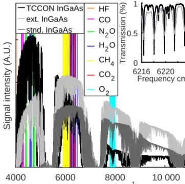
All TCCON sites employ the high-resolution Bruker Optics™ IR FT spectrometer (IFS) 125HR that has been described in detail elsewhere (Washenfelder et al., 2006; Wunch et al., 2011b). For the Caltech TCCON site (34.1362◦N, 118.1269◦W, 237 m a.s.l.), the IFS 125HR uses an extended InGaAs (indium gallium arsenide) detector, covering 3800–11 000 cm−1 for detection and retrieval of all gases relevant to this study (O2, CO2, CH4, CO, and
4000 6000 8000 10 000 Frequency (cm-1)
Signal intensity (A.U.)
HF CO N
2O
H
2O
CH
4
CO2 O2
6216 6220 Frequency cm-1 0
0.5 1
Transmission (%)
TCCON InGaAs ext. InGaAs stnd. InGaAs
Figure 1.Example of scaled spectra from three different detector types, with retrieval windows highlighted. The spectrum from the EM27/SUN extended InGaAs detector was scaled 10 times more than the spectrum from the standard InGaAs detector.
EM27/SUN instruments, with the spectral regions where in-dividual gases are retrieved highlighted. Oxygen (O2) abun-dance is useful in calculating the DMF because it represents the column of dry air and is combined with the column of the gas of interest to yield the DMF (Wunch et al., 2010).
The Caltech IFS 125HR uses a resolution of approxi-mately 0.02 cm−1(with a maximum optical path difference (MOPD) of 45 cm). It takes about 170 s to complete one for-ward/backward scan pair. TCCON sites have single sound-ing 2σuncertainties of 0.8 ppm (XCO2), 7 ppb (XCH4), 4 ppb
(XCO), and 3 ppb (XN2O)(Wunch et al., 2010). TCCON data
are tied to the World Meteorological Organization (WMO) in situ trace gas measurement scale through extensive com-parisons with in situ profiles obtained from aircraft and bal-loon flights. We use the TCCON as a standard against which to compare the EM27/SUN instruments. TCCON data from this study are publicly available from the Carbon Dioxide In-formation Analysis Center (Wennberg et al., 2014).
2.2 Caltech EM27/SUN
EM27/SUN spectrometers have been described elsewhere (Gisi et al., 2012; Frey et al., 2015; Klappenbach et al., 2015) so we focus on differences in setup and acquisition here. The standard EM27/SUN configuration uses an InGaAs detector sensitive to the spectral range spanning 5500–12 000 cm−1,
which permits detection of O2, CO2, CH4, and H2O (Frey
et al., 2015). For this study, the Caltech EM27/SUN was delivered with an extended-band InGaAs detector sensitive to 4000–12 000 cm−1, which allowed for additional mea-surements of CO and N2O (Fig. 1). All EM27/SUN
spec-trometers used in this study (Sects. 2.2, 2.3) used the typ-ical MOPD of 1.8 cm, corresponding to a spectral
reso-lution of 0.5 cm−1. Interferograms (ifgs) were acquired in direct-current-coupled mode to allow post-acquisition low-pass filtering of brightness fluctuations to reduce the impact of variable aerosol and cloud cover effects (Keppel-Aleks et al., 2007). Ghosts were reduced as data were acquired by employing the interpolated sampling option provided by Bruker™ (see also Sect. 4.3). A 10 KHz laser fringe rate is used to reduce scanner velocity deviations, and each for-ward/backward scan took 11.6 s, or 5.8 s per individual mea-surement.
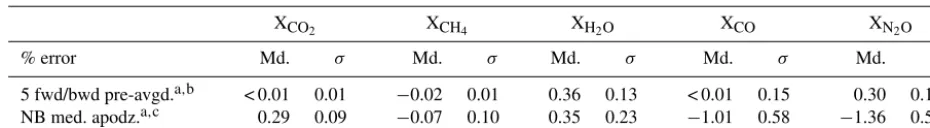
To be more consistent with the TCCON measurements, no spectrum averaging or interferogram apodization was ap-plied before retrieving DMFs. We recommend averaging only after retrievals if disc storage and processor speeds are sufficient, so spurious data can be filtered. To test the pre- vs. post-averaging effect we used 9 retrieval days with 26 000 forward/backward measurements and used Bruker™ OPUS software to create spectra from ifgs. We compared retrievals from using five combined backward/forward measurements averaged pre-retrieval with those averaged post-retrieval. We also compared combined forward/backward measurements using a medium Norton–Beer apodization with those using no special apodization. Results are in Table 1 and suggest that different averaging methods cause only small inconsis-tencies, under∼0.02 % for XCO2 and XCH4.
The EM27/SUN was placed within 5 m of the Cal-tech TCCON solar tracker mirrors on the roof of the Linde+Robinson building (Hale, 1935). Measurements started on 2 June 2014 and, for this study, we include 186 measurement days that end on 4 May 2015. About 800 000 individual EM27/SUN measurements and 40 000 in-dividual TCCON measurements were acquired over this period. Of these, about 580 000 and 15 000 were consid-ered coincident and were not screened out by our qual-ity control filters (QCFs). Our QCFs were conservative, and they required signal > 30 (Sect. 4.4), solar zenith angle (SZA) < 82◦, 370 ppm < XCO2< 430 ppm, XCO2,error< 5 ppm,
XCO,error< 20 ppb, and XCH4,error< 0.1 ppm. Other users may
consider stricter QCFs. After averaging data into 10 min bins, there were about 6500 binned comparison points.
2.3 LANL and Harvard EM27/SUN instruments
Table 1.Pre-averaging and apodization effects on EM27/SUN retrievals.
XCO2 XCH4 XH2O XCO XN2O
% error Md. σ Md. σ Md. σ Md. σ Md. σ
5 fwd/bwd pre-avgd.a,b < 0.01 0.01 −0.02 0.01 0.36 0.13 < 0.01 0.15 0.30 0.12 NB med. apodz.a,c 0.29 0.09 −0.07 0.10 0.35 0.23 −1.01 0.58 −1.36 0.55
Measurement compared over 1–10 July 2014. Md denotes the median. NB denotes the medium Norton–Beer apodization.aAs compared to retrievals from 1 fwd/bwd averaged non-apodized measurement averaged over same time post-retrieval.bSame apodization as standard.cSame pre-averaging as standard.
gas column amounts are retrieved in that region. The LANL instrument was first used in January 2014 and has been com-pared with multiple TCCON sites in the United States, in-cluding sites at Four Corners, LANL, NASA Armstrong, La-mont, Park Falls, and multiple Caltech comparisons (Parker et al., 2015). The HU instruments have been operational since May 2014 and were compared against each other at Harvard before traveling over 4100 km to Caltech. As noted by Gisi et al. (2012) and Chen et al. (2016), the ILS of these instruments is remarkably stable considering the long dis-tances they traveled.
3 Retrieval software
SFIT (Pougatchev et al., 1995), PROFFIT (“PROFile fit”, Hase et al., 2004), and GGG (Wunch et al., 2015) are the three widely used retrieval algorithms to fit direct so-lar spectra and obtain column abundances of atmospheric gases. PROFFIT is maintained by the Karlsruhe Institute of Technology (KIT) and has been used to obtain DMFs from EM27/SUN instruments as well as NDACC-IRWG sites (Gisi et al., 2012; Frey et al., 2015; Hase et al., 2015). GGG is maintained by the Jet Propulsion Laboratory (JPL) and has been used to obtain DMFs from other low-resolution instrument measurements (e.g., an IFS 66, see Petri et al., 2012), in addition to being used to retrieve DMFs from the MkIV spectrometer in balloon-borne measurements (Toon, 1991) and for the Atmospheric Trace Molecule Spectroscopy Experiment (ATMOS) flown on the space shuttle (Irion et al., 2002). GGG is the retrieval algorithm used by the TCCON (Wunch et al., 2011b). We chose to use GGG for our anal-ysis because (1) we want to be consistent with the TCCON for comparison and (2) the GGG software suite containing GFIT is open-source allowing us to adapt routines if needed. We used the GGG2014 version for retrievals (Wunch et al., 2015).
All retrievals used the same pTz and H2O modeled
pro-files as well as the same a priori propro-files (Wunch et al., 2015). We also used the same meteorological surface data for retrievals from all five instruments. All retrievals also used the same 0.2 hPa surface pressure offset. This offset was determined by comparing measurements from the stan-dard barometer with a calibrated Paroscientific Inc. 765–16B
Barometric Pressure Standard that has a stated accuracy of better than 0.1 hPa.
3.1 Interferogram-to-spectrum – double-sided
TCCON uses an interferogram-to-spectrum subroutine part of GGG to perform fast Fourier transforms (FFTs) to create spectra from ifgs (Wunch et al., 2015). Though the Bruker™ OPUS software used to operate the spectrometer can also perform FFTs, we again chose to use GGG to maintain con-sistency. A developmental version of GGG was used, which was adapted to also allow FFT processing on EM27/SUN interferograms. GGG splits a raw forward/backward ifg into two different double-sided ifgs which are then FFTed to yield two spectra. GGG also corrects source brightness fluctua-tions (Keppel-Aleks et al., 2007).
3.2 EM27/SUN GGG and interferogram processing
suite (EGI)
To make GGG retrievals simpler for new EM27/SUN users, an add-in software suite (EGI) was developed at Caltech to create correctly formatted input files. This suite is open-source and can be obtained through correspondence to the email address listed. EGI can be run using MATLAB or Python. EGI runs in UNIX, Mac OS, and Linux environ-ments and runs GGG on multiple processors. EGI central-izes settings for paths to read and write files, it coordinates separately acquired ground weather station and GPS data with EM27/SUN ifgs, and it optimizes processing order. It also provides some ancillary calculations such as a spectral signal-to-noise ratio (SNR) calculation. EGI provides a sim-ple way to turn on and off saving of ancillary retrieval files (i.e., spectral fits and averaging kernels). EGI can run for in-struments employing one or two detectors, such as the type described by Hase et al. (2016). Like the GGG software suite, EGI also includes benchmark spectra acquired under differ-ent conditions to run simple tests on. EGI is automated, re-ducing the learning time as well as the amount of user time needed to retrieve DMFs. After an initial setup, EGI will run from ifgs to retrieved Xgaswith two commands. On a
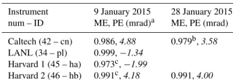
Table 2.ILS of EM27/SUN instruments. Instrument
num – ID
9 January 2015 ME, PE (mrad)a
28 January 2015 ME, PE (mrad)
Caltech (42 – cn) 0.986,4.88 0.979b,3.58 LANL (34 – pl) 0.999,−1.34
Harvard 1 (45 – ha) 0.973c,−1.99
Harvard 2 (46 – hb) 0.991c,4.18 0.991,4.00
Missing values indicate ILS not characterized on that day.aPhase error values are italicized.bAfter realigning this instrument the ME was as high as 0.994. cAs reported by Chen et al. (2016).
4 Instrument characterizations and performance
4.1 Instrument line shape
Knowledge of the instrument line shape (ILS), or the ob-served shape of a spectral line from a monochromatic input, is crucial in assessing instrument performance and avoiding unknown biases in retrievals. Two parameters in the the LIN-EFIT algorithm (Hase et al., 1999) are used to characterize the ILS in relation to an ideal instrument, namely the modu-lation efficiency (ME) and phase error (PE). ME and PE both describe the interferogram and vary with OPD (Hase et al., 1999; Frey et al., 2015). PE is the angle between the real and imaginary parts of the FT of the ILS (Wunch et al., 2007). PE has an ideal value of 0 radians, and indicates the degree of asymmetry in spectral lines. ME is a measure of the nor-malized observed interferogram signal compared with that of a nominal instrument with an ideal value of 1 (unitless) (Hase, 2012). At maximum OPD (MOPD), an ME < 1 causes a broadening of the measured spectral lines, while an ME > 1 at MOPD causes a narrowing. The ILS can be calculated by analyzing absorption lines measured through a low-pressure gas cell, and varies with OPD (Hase et al., 1999). Here, we use only single ME and PE values at the MOPD (Frey et al., 2015) to describe the ILS. We characterized the ILS for the EM27/SUN instruments using the method described else-where (Frey et al., 2015; Klappenbach et al., 2015). This method is able to characterize ME to within 0.15 % using the LINEFIT algorithm (Hase et al., 1999), with supplemen-tal MATLAB scripts for automation purposes (Chen et al., 2016). ILS can affect retrieved column values. We note that the ME at MOPD of the cn and ha instruments in Table 2 are significantly lower than those reported by KIT on campus of ∼0.997 (Frey et al., 2015), and post-campaign of∼0.996 (Klappenbach et al., 2015).
For this study, the ILS is used to help explain biases, to demonstrate the stability of the instruments, and gives insight into how well the EM27/SUN instruments are aligned and their optical aberrations. Though GGG2014 retrievals do not account for non-ideal ILS, future versions of GGG will. For the current study, we assume that ILS impacts using PROF-FIT will be similar to impacts using GGG. This assumption
5 10 15 20 25 30 35 40 Ambient temperature °C -120
-100 -80 -60 -40 -20 0
CO
2
6220 cm
-1 FS (ppm)
CIT EM27 LANL EM27 HU EM27 (1) HU EM27 (2)
Figure 2.Frequency shifts (FS) of all four instruments vary with temperature because the lasers are not frequency-stabilized. FS for the CO26220 cm−1window are shown. FS of the Caltech (CIT)
instrument are far from zero, so an empirical correction is made to correct the sample spacing number. Only every 300th CIT point and every 20th LANL point is plotted for clarity. HU EM27 1 and 2 are also referred to as ha and hb respectively by Chen et al. (2016).
will need to be tested when GGG also can account for a non-ideal ILS. Because future GGG retrievals will be revised us-ing historical ILS measurements, a need remains to monitor the ILS both for future retrievals and as an indicator if re-alignment is necessary.
4.2 Frequency shifts
EM27/SUN units contain a HeNe 633 nm (15 798 cm−1)
metrology laser to sample the IR signal accurately as a func-tion of the OPD. The laser is not frequency-stabilized (Gisi et al., 2012). This causes apparent spectral frequency to change with temperature as is shown in Fig. 2. Frequency shifts are affected by changes in the input laser wavenum-ber, laser alignment, and IR beam alignment. The input laser wavenumber will affect the spacing between spectral points. Since the frequency shift is furthest from zero for the Caltech EM27/SUN (on order of−100 ppm, in red Fig. 2), the spec-tral spacing is empirically corrected in the EGI suite based on the CO26220 cm−1window frequency shifts. This made
lit-tle difference for the primary gases of interest affecting XCO2
by 0.015 % and XCH4by−0.005 %, though it did affect XH2O
by 4 %.
4.3 Ghosts
prevent aliasing, the IR interferogram is sampled twice each laser interferogram cycle, on the rising and falling edge. However, if the laser sampling is asymmetric – for exam-ple from a faulty electronics board – aliasing can still occur, folded across the half laser frequency (Messerschmidt et al., 2010). Because the asymmetry is typically small, the aliased signal, or ghost spectrum, is small compared with the true spectrum (Dohe et al., 2013; Wunch et al., 2015).
In EM27/SUN instruments the laser sampling error (LSE) can be minimized as data are collected by employing the in-terpolated sampling option provided by Bruker™. This re-sampling mode uses only the rising edge of the laser interfer-ogram and assumes constant velocity in between the rising edges to interpolate the sampling (Gisi, 2014). We use a nar-row band-pass filter (3 dB band width 5820–6150 cm−1)in the Caltech EM27/SUN to test for LSE ghosts at 9800 cm−1. The ghost to parent ratio is 1.73×10⁻⁴at a 10 kHz
acqui-sition rate without the interpolated sampling activated. This ghost is eliminated with the interpolated sampling turned on. In actual solar tests, turning the interpolated sampling on and off had no noticeable effect on the DMF retrievals for the Caltech EM27/SUN; however this may not hold true for all instruments. The LSE ghost also disappeared at an ac-quisition frequency of 20 kHz, and returned at higher acqui-sition frequencies. We opted for the recommended 10 kHz acquisition rate with the interpolated sampling on for all EM27/SUNs in this analysis because other instruments may be more significantly affected by LSE ghosts. A double-frequency ghost remains at ∼11 900 cm−1 from radiation passing through the interferometer twice that is much larger than the LSE ghost, but is not in a region that will affect re-trievals.
4.4 Mirror degradation and detector linearity
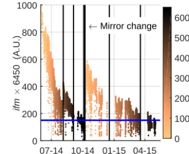
Solar tracking mirrors provided with the EM27/SUN instru-ments are gold with a protective coating. Gold is used be-cause of its excellent reflectance in the near-IR and low re-flectance in the visible region (Bennett and Ashley, 1965), which allows a high signal while reducing excess heating of the field stop and other optics. Through extended tests, we noted the first two mirrors (gold on plated aluminum, with a coating) degrade over time, with an e-folding degradation time of∼90 days as is shown in Fig. 3. Arbitrary units (AUs) for signal are the maximum ordinate values of the unmodi-fied interferograms multiplied by 6450. The AUs of signal happen to be close to the spectral SNR – a scaling factor of 1.3 applied to the arbitrary signal has anR2of 0.63 relative to the SNR. Cleaning helped restore some signal, but never to the original values. The mirror change may not have restored full signal because the rest of the optics were not cleaned at the time of the mirror change. Below the blue 150 AU line in Fig. 3 the fitted O2root mean square (rms) as a percentage of
the continuum level dropped 26 times faster with signal in-tensity than above it. The instrument did come with an extra
07-14 10-14 01-15 04-15 Month-year 0
200 400 600 800 1000
ifm
#
6450 (A.U.)
A Mirror change
0 100 200 300 400 500 600
Hours of sun observations
Figure 3.Interferograms from EM27/SUN instruments are nega-tive, with the most negative ordinate values at ZPD and saturation occurring at−1. Here the interferogram maximums (ifm) refer to the maximum (least negative) ordinate values of the raw interfer-ograms. They were normalized so the maximum is 1000 and are plotted with time showing the loss of signal. These values are af-fected by clouds, which are the cause for much of the scatter. They are also affected by SZA which explains some apparent interme-diate increases. Only every 50th point is plotted for clarity. Mirror cleaning (thin black lines) helped restore some signal, but never to original values. The 150 AU line is in blue.
set of mirrors, but because mirrors are consumable parts, it adds recurring cost and effort to maintain these instruments long-term. After 1 year of use, the third mirror (gold coated glass) still remains completely intact. Feist et al. (2016) had success using steel mirrors under the very harsh conditions at the Ascension Island TCCON site, though at a cost of 35 % reflectivity per mirror. The JPL TCCON sites near Caltech noted no degradation on the external gold mirrors over more than 1 year of measurements. The lack of degradation on the third external mirror and the JPL TCCON mirrors is likely due to differences in how the mirrors were manufactured, in-cluding how the gold is applied to the substrate and the coat-ings used. Mirror degradation has likely not been a widely re-ported problem for most of the EM27/SUN community, per-haps because these instruments typically are stored indoors and only used for a few days for campaigns (for example, Frey et al., 2015). However, this problem may affect mirrors on other EM27/SUN instruments when mirrors are exposed outside for extended periods of time.
With signal loss, we would anticipate that gas measure-ments would become noisier but remain unbiased. However, with time, the Caltech EM27/SUN XCO2 and XCH4 DMFs
decreased relative to the TCCON DMFs as mirror reflectance decreased, and XCO2 and XCH4 increased when the mirrors
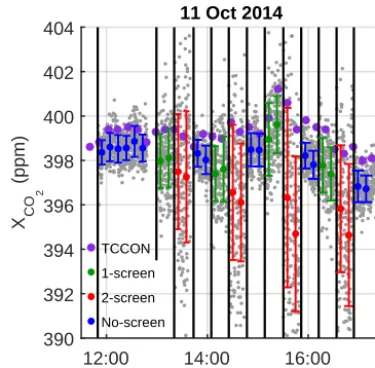
en-12:00 14:00 16:00 UTC-7
390 392 394 396 398 400 402 404
X CO
2
(ppm)
11 Oct 2014
TCCON
1-screen
2-screen
No-screen
Figure 4.XCO2retrievals on 11 October 2014 when mesh screens were repeatedly moved in front of and away from the EM27/SUN (with extended InGaAs detector) entrance window. Gray points are all EM27/SUN measurements. Large points are 10 min averages. Error bars are 1σ. This test was performed a few days after the mirrors were replaced.
trance window to filter some of the light. In these tests XCO2
and XCH4 changed on order of 3 and 0.01 ppm respectively
when using the extended InGaAs detector in the presence of filters transmitting∼25 % of the light. Figure 4 shows results from this test on XCO2; results from XCH4 are similar. This
provides strong evidence that the extended InGaAs detector is nonlinear. We repeated the test using the standard InGaAs detector, and changes in XCH4 and XCO2 biases were of the
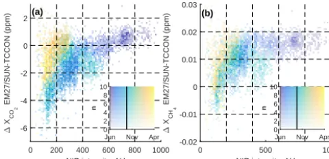
order of 10 times smaller and could be attributed to scatter-ing off the mesh screen placed in front of the entrance win-dow. Figure 5 shows the difference between the EM27/SUN and TCCON XCO2 and XCH4as the total signal changed.
Af-ter the mirrors were changed, the relative difference actually went up with some signal loss before decreasing again, for reasons we do not understand.
Detector nonlinearity in FTS instruments can be corrected in the ifgs post-acquisition in two ways. The first option deals with artifacts around the ZPD (zero path difference point) and is already included in GGG (Keppel-Aleks et al., 2007). When the ifg is smoothed, a nonlinear detector exhibits a dip around the ZPD which can be used to diagnose and reduce detector nonlinearity effects. EM27/SUN measurements are too noisy to properly characterize or detect this dip and so this correction is insufficient. The other option is to compare detector response with radiance from a controlled external light source, such as a blackbody, with very accurate radia-tion flux measurements (on order of 0.01 %) (Thompson and Chen, 1994). By characterizing the response to the true flux as it is varied, the detector can be characterized and ifgs can be appropriately scaled and corrected. However, this requires
extremely controlled precise measurements, as all nonlinear-ity is likely less than 1 %, so measurements must be more precise than 1 %.
An option to prevent nonlinearity from interfering with measurements is to only use the detector over its linear range by sufficiently attenuating the incoming sunlight. However, the SNR is already low so we opted against this method. Ul-timately, we purchased the non-extended InGaAs detector at the loss of CO, and N2O for future measurements for the
Caltech instrument. For the historical field measurements we use a bias correction to match the TCCON for the nearest comparison days. The nonlinearity has nearly an equal effect for short times, but has a larger variation on multi-monthly scales as the mirrors degrade. In future measurements we recommend against using these extended InGaAs detectors. Addition of band-pass filters or use of different detectors will be necessary to provide high-quality measurements of CO, CO2, and CH4(Hase et al., 2016).
The data shown in Fig. 5 were divided into bins based on the signal intensity and were separated before and after the mirror change. Within each bin the relationship was treated as approximately linear. Fits using fewer than 10 points or with correlation coefficients less than 0.1 were discarded. The change with half signal was calculated. The analysis was repeated for 10 bins and again for 20 bins. The weighted mean change in XCO2 for halving the signal is−1.43 ppm
in agreement with the mesh tests or
1XCO2
ppm−1=2.06 ln(S/S0) , (2) where S and S0are the final and initial signals respectively.
This relationship holds for S and S0in the middle 80 %. For
a similar methane analysis the mean change for half signal is −7.25 ppb or
1XCH4
ppb−1=10.5 ln(S/S0) . (3)
5 Comparisons with Xgas
GGG2014 includes an air-mass-dependent correction factor derived for TCCON Xgas measurements. The air mass
cor-rection factor for each gas is calculated using data obtained at a variety of relatively clean sites as described by Wunch et al. (2011b). We expect that the air mass dependence, which is due primarily to spectroscopic uncertainties, should be com-mon for the same type of measurement. Parker et al. (2015) noted that the average EM27/SUN factors are similar com-pared to the TCCON for XCO2 at three clean sites in the
United States. The XCH4 β factor was different (−0.0077
EM27/SUN, 0.0053 TCCON) but when applied here it wors-ened theR2and standard deviation of the comparisons. This could be because the air mass dependence of XCH4 may not
0 200 400 600 800 1000 NIR intensity, AU -6 -4 -2 0 2 " X CO 2 EM27/SUN-TCCON (ppm) (a)
Jun Nov Apr
0 2 4 6 8 10 n
0 500 1000
NIR intensity, AU -0.02 -0.01 0 0.01 0.02 0.03 " X CH 4 EM27/SUN-TCCON (ppm) (b)
Jun Nov Apr
0 2 4 6 8 10 n
Figure 5. (a)The XCO2retrieved from the EM27/SUN compared to TCCON decreased with signal intensity for the first set of mirrors. In October the mirrors were changed, which caused the retrieved XCO2 to increase. The inset is the legend for the average date and number of points in the histogram bins.(b)XCH4retrieved from the EM27/SUN compared with TCCON.
To compare measurements between the TCCON and the EM27/SUN instruments, data were first averaged into 10 min bins to reduce the variance of binned differences (Chen et al., 2016). The median of the XCO2 differences
be-tween sequential time bins is smallest (around 0.26 ppm) for 10 min bins over the entire ∼11 month time period. Less averaging is more affected by noise, and more averaging starts to include instrument drift and true atmospheric vari-ations. Averages were weighted using retrieval errorsxˆerras
in Eq. (4):
ˆ x=
P
i ˆ xixˆ−i,err2
P
i ˆ
x−i,err2 , (4)
wherexˆi is the retrieved value from theith measurement in
a bin, andxˆ is the bin average.
5.1 Averaging kernels
When comparing retrieved Xgasmeasurements (also denoted
ˆ
c)from different remote sensing instruments, differences in their averaging kernels (AKs or ai, where i represents an
instrument indicator number) and a priori profiles must be taken into account, using for example, the methods described by Rodgers and Connor (2003). Wunch et al. (2011a) com-pared GOSAT and TCCON total column DMFs using this method. Because GGG scales a priori profiles rather than re-trieving the full profile, these AKs are vectors (i.e., column averaging kernels) rather than matrices.
Averaging kernels depend on several factors including how strong the lines are in the retrieval windows, and view-ing geometry (e.g., SZA for solar-viewview-ing instruments). Be-cause the TCCON IFS 125HR and EM27/SUN instruments have different spectral resolutions, the apparent absorption strengths are different and so are the averaging kernels. Av-eraging kernels for a gas differ for each microwindow. We
0 0.5 1 1.5 2 AK 100 200 300 400 500 600 700 800 900 1000 Pressure (hPa) CO 2
0 0.5 1 1.5 2 AK
CH
4
0 0.5 1 1.5 2 AK
CO
0 0.5 1 1.5 2 AK N 2O 100 200 300 400 500 600 700 800 900 1000 Pressure (hPa)
CO2 CH4 CO
N 2O 0 10 20 30 40 50 60 70 80 90
SZA (°)
Figure 6.Top row: averaging kernels from the Caltech EM27/SUN instrument. Bottom row: averaging kernels from the TCCON.
combined AKs of a given gas from different microwindows using an unweighted average. Averaging kernels for the Cal-tech EM27/SUN for the GGG retrieval windows are shown in Fig. 6. Averaging kernels from the other EM27/SUN in-struments are similar. TCCON averaging kernels have been discussed by Wunch et al. (2011b) and are shown on the bot-tom row in Fig. 6. As a numerical example, for XCO2
mea-sured at 50◦SZA and 900 hPa using GGG, the AK is 1.10 for EM27/SUN instruments and 0.93 for TCCON instruments. This means EM27/SUN instruments are slightly more sensi-tive to a change in CO2near the surface relative to TCCON
instruments. More importantly, they have the opposite sensi-tivity to an error in the a priori volume mixing ratio (VMR) profile at 900 hPa.
In our particular case, reducing the smoothing error us-ing Eq. (A13) from Wunch (2011a) and usus-ing the a priori as the comparison ensemble changes little as the effect of the differences in averaging kernels from the top of the at-mosphere tends to cancel out the effect of differences at the bottom. TCCON and EM27/SUN a priori profiles were the same in this comparison. However, we need to consider that the a priori profiles used in the retrieval are not representa-tive of a highly polluted place, such as Pasadena, which is located in the same air basin as Los Angeles. Because dif-ferences in column measurements compared to background or a priori profiles occur primarily because of differences at the surface we can adjust retrievals for one instrument taking into account this knowledge using
ˆ
c1=a1,s
a2,s
ˆ
c2−ca+ca. (5)
Definitions of the terms in, as well as a discussion of assump-tions needed to obtain Eq. (5) are in Appendix A. We applied Eq. (5) to the XCO2 and XCH4 retrievals.
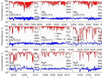
knowl-5900 5940 5980 -20 0 20 40 60 80 100 Transmittance, % CH4 rms=0.22 %
6020 6060 6100 6140
CH4
rms=0.17 %
6200 6220 6240
CO 2
rms=0.19 %
6300 6320 6340 6360 6380
CO 2
rms=0.19 %
4220 4230 4240 4250
CO
rms=0.27 %
4270 4290 4310
8 (cm-1)
-20 0 20 40 60 80 100 Transmittance, % CO rms=0.32 %
4380 4390 4400 4410 8 (cm-1)
N 2O
rms=0.19 %
4700 4720 4740 8 (cm-1)
N 2O
rms=0.28 % 7800 7850 7900 7950 8000
-20 0 20 40 60 80 100 Transmittance, % O 2 rms=0.20 % Meas. Fit Resid.#20
CO2 H2O N2O Other Solar
CO2 H2O HDO Other Solar H2O HDO CH4 Other Solar H2O
HDO Other Solar
CH4 H2O HDO Other Solar CH4
H2O HDO Other Solar
CH4 H2O HDO Other Solar CH4
H2O CO2 Other Solar 0O2
H2O HF CO2 Other Solar
Figure 7. Example spectral fits and residuals (×20) from several of the retrieval windows from 28 June 2014, 10:55:16 (UTC−8), SZA=17.1◦. The primary species of interest and root mean square (rms) of the residuals are listed on the left. Other species fit in the window are listed on the right.
edge of the atmospheric profile and differences in averaging kernels.
5.2 Full comparisons of Xgasfrom extended-band
InGaAs detector with a TCCON site
Gisi et al. (2012) noted that measurements taken within the first 30 min of moving the instrument to the roof and turn-ing it on needed to be filtered out because of high scatter while waiting for the instrument to operate stably. We did not observe a similar requirement for our data. This could be because our instruments were not subjected to such fast temperature changes. It could also be because the laser fre-quency shift, which changes with temperature, does not seem to significantly impact our retrievals.
Examples of spectral fits from several of the retrieval win-dows are shown in Fig. 7 for a single spectrum. These are not necessarily representative of all the conditions under which the 800 000 spectra were acquired. The residuals are larger than those reported by Gisi et al. (2012) and Frey et al. (2015) because of the lower SNR from spectra recorded using the extended InGaAs detector.
The full time series (186 days) of the difference be-tween the Caltech EM27/SUN and TCCON measurements is shown in Fig. 8. From this figure we see that XCO2 and
XCH4are the gases most affected by the mirror change in
Oc-tober 2014 (by about 3 ppm and 12 ppb respectively). For all
gases, scatter of retrieved Xgasincreases as signal decreases.
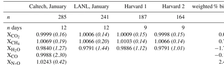
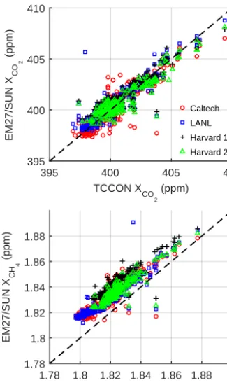
Figure 9 shows the retrieved XCO2 and XCH4 from all four
EM27/SUN instruments for 9–12 days in January 2015 plot-ted against those from TCCON. We report biases for Jan-uary 2015 as scaling factors to approximate to the TCCON, or scaling factors compared to 1. Biases were calculated us-ing a linear least squares fit forced through the origin. A sum-mary of the biases for all gases as compared to the TCCON is provided in Table 3.
5.3 XCO2
We note a smaller bias in XCO2 with respect to the TCCON
(+0.03 %, see Table 3) compared to previous EM27/SUN studies (Gisi et al., 2012; Frey et al., 2015; Klappenbach et al., 2015). These previous studies retrieved Xgas from
EM27/SUN spectra using PROFFIT. When compared with the TCCON XCO2 retrievals, Gisi et al. (2012) noted a +0.12 % bias, Frey et al. (2015) noted a+0.49 % bias, and Klappenbach et al. (2015) noted a+0.43 % bias. Reasons for these differences could be from (1) spectroscopy differences between PROFFIT and GGG2014 used for EM27/SUN Xgas
Table 3.EM27/SUN to Caltech TCCON biases.
Caltech, January LANL, January Harvard 1 Harvard 2 weighted % bias
n 285 241 187 164
ndays 12 12 9 9
XCO2 0.9999 (0.16) 1.0006 (0.14) 1.0009 (0.15) 0.9998 (0.15) 0.03 XCH4 1.0069 (0.19) 1.0066 (0.20) 1.0103 (0.14) 1.0066 (0.14) 0.75 XH2O 0.9840 (1.27) 0.9791 (1.44) 0.9886 (1.12) 0.9791 (1.01) −1.73
XCO 0.9988 (2.30) −0.12
XN2O 1.0243 (0.42) 2.43
Italicized values in parentheses are percent standard deviations as compared to the TCCON over the dataset for January 2015.
-5 0 5
"
O 2
(m
o
lc
c
m
-2 ) #10
22 EM27/SUN - TCCON
-5 0 5
"
XCO
2
(p
p
m
)
-0.02 0 0.02
"
X CH
4
(ppm)
-10 0 10
"
X CO
(ppb)
-10 0 10
"
X N
2
O
(ppb)
Jun Jul Aug Sep Oct Nov Dec Jan Feb Mar Apr May -200
0 200
"
X H
2
O
(ppm)
4.473e+24
400.0
1.821
90.9
315.7
2430.1
Figure 8.Full time series of EM27/SUN measurements as compared to TCCON from June 2014 to May 2015. Thin vertical gray lines represent mirror cleaning. The thick line represents the mirror change. To the right are TCCON means over time to get a sense of percent deviations.
section, we investigate two possible causes of bias: spectral resolution and instrument line shape.
Following Gisi et al. (2012), we attempted to determine whether the cause of the bias is due to the difference in spec-tral resolution between the EM27/SUN and TCCON instru-ments. Petri et al. (2012) also considered resolution bias in their study using a 0.11 cm−1resolution instrument and an older version of GGG. They did not report a bias in XCO2
re-trievals, but noted that XCO2decreased by∼0.12 % as
inter-ferograms were truncated to obtain spectra with resolutions of 0.02 to 0.5 cm−1. Most of the change occurred as the reso-lution changed from 0.1 to 0.5 cm−1(see Fig. 11 therein). In contrast, Gisi et al. (2012) noted a 0.13 % increase in XCO2as
the resolution changed from 0.02 to 0.5 cm−1 in PROFFIT. Here we find a 0.08 %±0.16 % (1σ )decrease in XCO2 when
the resolution is decreased from 0.02 to 0.49 cm−1in GGG, though part of this change would be offset by considering the differences in averaging kernels.
Previous studies noted an increase in XCO2 of 0.15 % for
a 1 % increase in modulation efficiency at max OPD (Gisi et al., 2012; Frey et al., 2015). Using PROFFIT we per-formed a similar test for spectra taken under various condi-tions at various times of day and obtained a similar result of a 0.10 %±0.02 % (1σ )increase in XCO2 for a 1 % increase
in ME at the MOPD. For this study we assume that impacts of the ILS on retrievals will be similar in GGG and PROF-FIT. Though we report a single value, there is an air mass dependence of∼0.05 % increase in EM27/SUN PROFFIT retrievals for a 1 % increase in ME and air mass change of 1. For instruments using the standard InGaAs detectors, the XCO2 10 min running 1σ precision is 0.075 % [0.034 to
pre-395 400 405 410 TCCON X
CO
2
(ppm) 395
400 405 410
EM27/SUN X
CO
2
(ppm)
Caltech LANL Harvard 1 Harvard 2
1.78 1.8 1.82 1.84 1.86 1.88 TCCON X
CH
4
(ppm) 1.78
1.8 1.82 1.84 1.86 1.88
EM27/SUN X
CH
4
(ppm)
Figure 9.Retrieved EM27/SUN measurements (10 min averaging) as compared to the TCCON from January 2015. This provides a visual representation of the data – offset and scatter of data between Xgasfrom different instrument types – in Table 3. The black dashed
line is the 1:1 line.
cision for XCO2 retrievals was only weakly correlated with
1/
√
SNR. Chen et al. (2016) found that the 1σ XCO2
pre-cision among 10 min binned EM27/SUNa-EM27/SUNb
dif-ferences is 0.01 %. These data were acquired in a way that about 67 spectra were acquired every 10 min, and because two instruments were used, the single sounding precision is ∼0.01 %×√67/2≈0.058 %, which falls in our measured running 1σ precision range. Comparing to the TCCON, Gisi et al. (2012) reported that the 1σ daily precision is 0.08 %. The extended InGaAs detector naturally has a lower spectral SNR, in the range 100–1000, with a median of 400 over the full time series. Most of the variation in the SNR is due to loss of mirror reflectivity, but even with non-degraded gold mirrors, it is∼5 times lower because of the different detec-tor. The median running 1σprecision over the full time series is 0.26 % for the XCO2 product from the extended InGaAs
detector. Because the SNR changed with time due to loss of mirror reflectivity, so did the precision. The correlation be-tween 1/
√
SNR and running 1σ XCO2 precision was strong
(R2=0.75) for retrievals from this detector and followed
σXCO2 =0.17+
8.4 √
SNR−57. (6)
An additional study we have not performed that could help in reducing bias would be to omit all or part of a CO2
win-dow with strong water lines. Because of the low resolution of these spectrometers (see inset Fig. 1), water lines and CO2
lines often overlap. This can lead to inaccurate retrievals de-spite a good overall fit because H2O and CO2can both be
wrong, but in compensating ways. Reducing the size of a window would reduce precision but would decrease water and temperature sensitivity. This adjustment could also be performed for CH4, which is retrieved over three windows in
GGG.
5.4 XCH4
The EM27/SUN XCH4 retrievals are 0.75 % higher than
those of TCCON (see Table 3). In previous work, high biases of 0.47 % for a 0.11 cm−1 instrument (Petri et al., 2012), and 0.49 % (Frey et al., 2015) and 1.87 % (Klap-penbach et al., 2015) for EM27/SUNs, were noted. Petri et al. (2012) attributed most (0.26 %) of their bias to differ-ences in resolution and noted for a single day that the bias increased as resolution decreased. In our simulations we find a 0.28 %±0.20 % (1σ ) increase in XCH4 when the
resolu-tion is reduced from 0.02 to 0.49 cm−1. Using PROFFIT the impact of a 1 % decrease in ME is a 0.15 %±0.01 % (1σ )
increase in XCH4. Again, although we report a single value
there is an air mass dependence of about a 0.12 % decrease in XCH4 using PROFFIT retrievals for an air mass change of
1, and a 1 % decrease in ME. Resolution and ME combined account for only half of the observed methane bias. Petri et al. (2012) suggested improper dry air mixing ratio and pT profiles, or spectroscopy as sources of error. Improper sur-face pressure, error in the calculated Observer-Sun Doppler Stretch (OSDS) due to pointing errors coupled with solar ro-tation, or error in the assumed field of view (FOV) may also contribute to the bias (see Sect. 6).
Chen et al. (2016) found that the 1σ XCH4 precision
among 10 min binned EM27/SUNa-EM27/SUNbdifferences
is 0.01 %, which is equivalent to a single sounding 1σ preci-sion of∼0.058 %. Using the same method as for XCO2, the
XCH4 running 1σ precision from instruments using the
stan-dard InGaAs detectors is 0.057 % [0.037 to 0.25 %, 95 % CI], in agreement with Chen et al. (2016). The median running 1σ
precision for XCH4 from instruments using the extended
In-GaAs detector is 0.33 %. XCH4 precision from the extended
InGaAs measurements is also correlated with 1/
√ SNR.
5.5 XCOand XN2O
XN2O and XCO were also measured using an EM27/SUN
spectrometer in this study. Hase et al. (2016) have also re-ported on XCOmeasurements using an EM27/SUN modified
because the extended detector is sensitive to the region 4200– 4800 cm−1, which contains useful windows where N
2O and
CO molecules absorb IR radiation. Both the XCOand XN2O
retrievals are highly sensitive to changes in the modeled tem-perature profile. The nonlinearity of the detector had a less pronounced effect on XCO and XN2O retrievals than it had
on XCO2 and XCH4 retrievals (Fig. 8). XCO and XN2O also
have poorer precision than XCO2and XCH4, so any
nonlinear-ity effect could be less than the noise. The 4200–4800 cm−1 spectral region is also affected differently from the nonlinear-ity than the 5000–7000 cm−1region where column CH4and
CO2 are retrieved; the continuum levels changed more for
the latter region. This may also explain in part why there is no noticeable change in XCOand XN2Owith signal. For XCO
the median 1σprecision is 3.7 %. In our simulations reducing the spectral resolution from the TCCON (0.02 cm−1)to near the EM27/SUN (∼0.5 cm−1), X
COdecreases 2.5 %±4.2 %
(1σ ) in low-resolution spectra, and at Caltech this change varies with time.
In general, as is seen in Fig. 8, XN2Oretrievals were highly
scattered and had a large offset from TCCON. In our simu-lations, reducing the resolution from TCCON (0.02 cm−1)
to EM27/SUN (0.5 cm−1)decreased XN2Oby 1.5 %±0.6 %
(1σ ). Retrievals from the 4430 cm−1 window were low (∼6 %), while the 4719 and 4395 cm−1regions were biased slightly high (∼1 %). The retrievals from the 4719 cm−1 re-gion additionally had some long-term trends for reasons we do not understand. For XN2O the median 1σ precision is
1.9 %.
5.6 XH2O
Because of the significantly lower spectral resolution of the EM27/SUN spectrometers, the spectral band widths for the H2O retrievals were increased as compared to the standard
TCCON approach (Wunch et al., 2010). For lower resolution spectra, the H2O lines appear much broader and the observed
transmittance is much lower at the edges of standard TC-CON spectral window. Thus, the spectral ranges of the low-resolution windows were expanded. Some of the standard TCCON windows used to retrieve H2O had too few spectral
points from the low-resolution instrument for good fits and were omitted. When expanding the windows, we ensured that no lines were admitted that made the effective ground-state energy E00 greater than∼400 cm−1. This reduces the tem-perature sensitivity to the modeled temtem-perature profiles. As with the TCCON windows, we tried to keep a wide range of H2O line strengths to accommodate large seasonal and
site-to-site variations of the H2O column. Windows were kept as
wide as possible without encountering large spectral fitting residuals.
For XH2O, we find a median 1σ precision of 1.9 % from
the instrument using the extended InGaAs detector. For in-struments using the standard-InGaAs detectors, the XH2O1σ
precision is 0.81 % [0.36 to 2.12 %, 95 % CI].
1 deg N1 deg E2 deg N2 deg E
1 day prior5 deg E5 deg N
10 days prior5 days prior100 days prior -2
-1.5 -1 -0.5 0 0.5
"
XCO
2
(ppm)
'Full <
'Md(<daily)
'<(Mddaily)
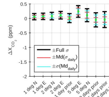
Figure 10.Standard deviations and biases from using wrong model pTz and H2O profiles as compared to using the standard option for
time and location. Tests are in order of increasing fullσ. Red repre-sents intraday variability. Cyan reprerepre-sents interday variability.
6 Sensitivity tests on retrievals
As with the TCCON, EM27/SUN retrievals require modeled atmospheric pressure, temperature, altitude (pTz), and wa-ter profiles (Wunch et al., 2015). Here atmospheric profiles are generated from the NCEP/NCAR 2.5◦reanalysis product (Kalnay et al., 1996) by interpolating to the correct location at local noon of the desired day. These profiles also include the tropopause height which is used to vertically shift a priori profiles, as tropopause height can significantly affect column DMFs such as XCH4 and XHF(Saad et al., 2014). Selecting a
profile for an incorrect location or day could lead to errors. We ran test retrievals for the July 2014 period with incor-rect profile information derived separately at latitudes north (1, 2, and 5◦) and longitudes west (1, 2, and 5◦) of our ob-servation site, and well as from profiles derived 1, 5, 10, and 100 days prior to the measurement dates. In general, the profiles generated from a more distant location in space and time caused larger retrieval errors. For XCH4 and XCO,
the main variability from the standard retrievals was in daily offsets (standard deviation of daily medians σ Mddaily)
which had values of 3 and 4 ppb respectively for the 100 day prior model. The medians of daily standard deviations
Md σdaily were 0.5 ppb for both XCH4 and XCO for the
100 day prior model. XN2O and XH2Oalso had more errors
fromσ Mddaily, except for profiles within 2◦, which more
strongly affected diurnal variability Md σdaily. For these
two species, the 100 day prior modelσ Mddailywere 2 ppb
and 50 ppm and Md σdailywere 1 ppb and 20 ppm
respec-tively. These values are shown for XCO2 in Fig. 10 for all
tested models. The 100 day prior model hadσ Mddaily
= 0.16 ppm and Md σdaily
Table 4.Meteorological sensitivity tests on EM27/SUN retrievals.
XCO2 XCH4 XCO XN2O
Error Offset Daily Offset Daily Offset Daily Offset Daily
+1 hPa surf 0.032 0.004 0.036 0.010 0.10 0.14 0.06 0.18
+10 K (surf – 700 hPa) 0.257 0.076 −0.006 0.036 10.1 1.2 0.53 0.23
Errors expressed as percentages. Daily is the median of the daily standard deviations, Mdσdaily
.
Table 5.Perturbations used in uncertainty budget.
Perturbation Magnitude
apavolume mixing ratio (VMR) downshift by 1 kmb ap temperature +1 K all altitudes ap pressure +1 hPa all altitudes Pointing offset (po) increased by 0.05◦
Surface pressure +1 hPa
Calculated OSDSc +2 ppm
Field of view (FOV) +7 %
See also Fig. 11.aap denotes a priori.bap VMRs were shifted independently. For XH2Oand XHDO, concentrations were decreased by 50 % at all levels.cOSDS=observer sun Doppler stretch.
X CO
2
% difference
-0.05 0 0.05
0.1 0.15 0.2 0.25
20140709 ap vmr ap temp ap pres pt offset
surf pres OSDS FOV
SZA (°)
0 10 20 30 40 50 60 70 80 90
XCH
4
% difference
-0.1 0 0.1 0.2 0.3
Figure 11.Uncertainty budget for EM27/SUN instruments using GGG2014. See Table 5 for magnitudes of perturbations.
Various user, instrumental, and measurement errors can reduce the accuracy and precision of retrievals. GGG uses retrieved O2 column amount with the average DMF of O2
(0.2095) to calculate the dry pressure column of air. How-ever, to calculate the O2absorption coefficients, GGG takes
into account the surface pressure, which can lead to mea-surement inaccuracies if the wrong surface pressure is used. Wunch et al. (2011b) reported a 0.04 % XCO2 bias for a +1 hPa surface pressure offset in the TCCON. Similarly, we find a 0.032 % XCO2 bias per+1 hPa surface pressure
off-set, with a 0.004 %σ variation on average throughout a day. Because the pressure offset affects O2 retrievals, the other
species are also affected (Table 4). XCOmay be particularly
affected by a pressure bias because such a large fraction of the column CO is near the surface.
Using the same July 2014 dataset used to test the sensi-tivity of the retrievals to error in the pTz profile and sur-face pressure, we further estimated the sensitivity to error in the temperature in the lower atmosphere (surface – 700 hPa). GGG uses a single temperature profile per day that repre-sents the local-noon temperatures, and the surface tempera-ture is extracted from that profile. Such temperatempera-ture error can arise in particular at the beginning and end of the day when the temperature is typically cooler than at noon. Here we de-rived the sensitivity of the retrievals to a+10 K error in the lower atmosphere (Table 4). XCO has a significantly larger
bias than the other species, likely because water absorption lines are the strongest spectral features in the CO retrieval window and water absorption lines are highly sensitive to changes in temperature. Water lines are also much stronger than N2O lines in the N2O windows. These tests suggest that
offsets under 1 hPa and 1 K would cause small (∼0.1 ppm) biases on XCO2, but a 4 K difference in near-surface (ground
– 700 hPa) temperature could cause∼0.4 ppm bias in XCO2
which is larger than our reported 1σ precision. For other studies using multiple spectrometers and multiple meteo-rological measurements for Xgas retrievals, we recommend
cross-comparing meteorological measurements to eliminate bias – preferably to a standard.
Finally, we perform a sensitivity study following the methodology of Wunch et al. (2015). The magnitudes of the applied perturbations are in Table 5. The results of this uncertainty budget study are presented for a day for XCO2
and XCH4 in Fig. 11. We do not include a sum in
TC-Table 6.Tests for assessing biases and sensitivities of solar-viewing, remote sensing instruments. Assessment Test/observation Type Accepted
correctiona
Root cause Similar instr. effect EM27/SUN test
Incoming radiation attenuation effect
Gray filter after solar tracker & before inter-ferometer
M Recom’d replace detector. Alt. empirical
Detector nonlinearity Consistent for same de-tectors
Sect. 4.4
ILS Measure with low-p gas cell (preferred), stable laser, or ambient air (least recom’d)
M Retrievals with non-ideal ILS
Instrument misalign-ment; in-built
Potentially large differ-ences
Gisi et al. (2012); Chen et al. (2014); Frey et al. (2015); Sects. 4.1 (measured), 5.3, 5.4 (impacts)
Adjust FOV (if ILS is measured but not ac-counted for in retrieval)
RIA Not recom’d
Ghost to parent ratio Use blackbody source & narrow band filter post-interferometer
M Laser mis-sampling Likely similar, poten-tially large diffs
Gisi et al. (2012); Frey et al. (2015); Sect. 4.3
Ghost effects Measurements with & without ghost correc-tion (e.g., XSM, or ifg resampling before FFT)b
M or RIA Recom’d interpol. during acq or post-resampling
Laser mis-sampling Likely similar, poten-tially large diffs
Sect. 4.3
Frequency shifts Changes or large 0 off-set
O & RIA Input spectral spac-ing
Improper laser wavenumber, mis-alignment of laser or NIR beam
Shifts differ, effect sim-ilar
Sect. 4.2
Solar gas stretch Changes or large 0 off-set
O & RIA OSDS Poor spectral fits of so-lar lines; SE or res.
Similar for same detec-tor & res.
Sect. 6
Spectral fitting windows
Width, locations RIA Instrument resolution requires adaptation
Same for similar res. (widths) & detector (lo-cations)
Gisi et al. (2012); Sect. 5.7 (H2O) Sect. 5.3 (discussion) Averaging kernels Used when comparing
with a different instru-ment type
O Rodgers and Con-nor (2003) and prior info.
Diff. sensitivity at at-mos. layers from differ-ing resolutionsb& VG
Same for similar res., microwindows & VG
Sect. 5.1
SZA artifacts Multi-day measure-ments in clean location
O Empiricala(Wunch et al. 2011b)
ILS, or SE See ILS entry Frey et al. (2015); Parker et al. (2015) Long-term artifacts Preferred co-location
with accepted measure-ments (e.g., TCCON)
O Various (e.g.,
instru-ment settling, changing alignment, other)
May widely differ Herein – for extended InGaAs only Region/zone dependence Co-location with spatially distributed accepted measurements
O/M A priori insufficiencies Likely similar Parker et al. (2015)
Surface pressure effects Manually adjust pres-sure inputs.
RIA Accurate barometer pres. calibr.
Poor calculation of O2 column, directly or by poor fitting
Similar effects for simi-lar resolutions
Sect. 6
pTz & H2O model profile sensitivity
Adjust modeled meteo-rological profiles
RIA Improve met. pro-files
Non-representative pTz+H2O profile
Similar effects for simi-lar resolutions
Sect. 6
A prori VMR surface sensitivity
Adjust a priori VMR near surface
RIA Improve a priori profiles; reduce effect with AKs
Non-representative VMR profile (e.g., polluted mixed layer)
Similar effects for sim-ilar res. & true VMR profile
Parker et al. (2015)
Opt. avg. time Allan type plot; e.g., Chen et al. (2016)
O Empirical SNR & true atmo-spheric variation
Depends on SNR & lo-cation
Chen et al. (2016) Sect. 5 Resolution effects Truncate
high-resolution ifg
RIA Apply offset Inst. res. Similar for all solar-viewing insts.
Gisi et al. (2012); Petri et al. (2012) Sects. 5.3–5.6 Uncertainty budget
for current fitting algorithm
Various, test on each new algorithm (Wunch et al. 2015)
RIA Informative Various Similar effects for simi-lar resolutions
Sect. 6
M denotes measurement (setups/adjustments required before acquisition), RIA denotes retrieval input adjustment (post-data acquisition, pre-retrieval), O denotes observation post-retrieval (may require prior planning of locations of measurements or longer term measurements), SE denotes spectroscopy errors, VG denotes viewing geometry, res denotes resolution.
aThough empirical corrections are occasionally accepted, it is always recommended to correct the underlying problem(s) if possible. bXSM is Bruker™code for interpolation during acquisition.
-5 0 5
"
O 2
(molc
cm
-2 ) #10
22 EM27/SUN - LR IFS 125
-5 0 5
"
X CO
2
(ppm)
-0.02 0 0.02
"
X CH
4
(ppm)
-20 0 20
"
XCO
(ppb)
-20 0 20
"
X N
2
O
(ppb)
Jun Jul Aug Sep Oct Nov Dec Jan Feb Mar Apr May
-200 0 200
"
XH
2
O
(ppb)
4.482e+24
399.5
1.826
87.0
311.3
2726.1
Figure 12.Time series comparison of EM27/SUN retrievals to retrievals from the 0.5 cm−1resolution IFS 125HR spectra.
CON that are unrelated to signal (e.g., Fig. 8, October– November 2014). For example, surface pressure and calcu-lated Observer-Sun Doppler Stretch (OSDS) were correcalcu-lated with EM27/SUN to TCCON XCO2 differences in the
long-term measurement. However, there was no apparent trend in the spectral residuals from fitting solar lines as the OSDS changed so these correlations may not indicate cause.
Differences in Xgasbetween different instruments are due
to a combination of differences in resolution, and real instru-mental imperfections and instabilities. To attempt to distin-guish between resolution causing differences (e.g., by limi-tations in the forward model) or instrumental issues, we re-peat the test performed by Gisi et al. (2012, Fig. 11 therein) of truncating IFS 125HR interferograms for the full time se-ries. Results are shown in Fig. 12. Mean values for XCO2 are
slightly lower because of differences from retrievals on spec-tra of different resolutions, as described in Sect. 5.3. When comparing 10 min averaged TCCON data with lower reso-lution IFS 125HR retrievals we note monthly standard de-viations on order of 0.15 % for XCO2 and XCH4. This
sug-gests the standard deviations of comparing retrievals from the EM27/SUN with the TCCON (Table 3) on these timescales are close to the current precision limits for directly compar-ing XCO2 and XCH4 retrieved from spectra of these
differ-ent resolutions. Results in Fig. 12 are slightly more scattered than in Fig. 8 and have different offsets. The data still show an increase in XCO2 and XCH4 in October–November 2014
for reasons we do not understand, and unfortunately we have no ILS characterizations over this period.
Long-term drifts may or may not affect instruments em-ploying the standard InGaAs detector and may be elimi-nated by future retrieval updates. They may also arise in part from how the comparison was made, e.g., the assumptions
to derive Eq. (A4) may not be valid for CH4 and N2O. As
a follow-up study, brief 5–6 day comparisons using a stan-dard InGaAs detector were made for the months of August, September, and November 2015. Scaling factors varied from 0.99905 to 1.00001 for XCO2 and from 1.01228 to 1.00893
for XCH4, with larger day-to-day variability. Long-term (1
year or more) comparisons of these instruments employing the standard-InGaAs detector are needed before claims of long-term accuracy can be made or the full magnitude of drift can be quantized. Errors that could lead to drifts likely would be correlated amongst all EM27/SUN instruments, so the comparison would need to be against a standard such as the TCCON. Future studies may also benefit from compar-ing results uscompar-ing different retrieval algorithms, as the magni-tude of errors that may lead to drifts in Xgasmay vary among
algorithms. Meanwhile, operators have already found many purposeful ways to use these instruments that require only short-term (about 1 month) precision without any assump-tions about precision for longer time periods (for example Hase et al., 2015; Chen et al., 2016; Viatte et al., 2016). Stud-ies using these spectrometers independently longer term can also be performed depending on the degree of precision re-quired. Limits on precision described herein are likely to only improve in future work.
7 Conclusions
Despite the challenge associated with the extended InGaAs detector and mirror degradation, the EM27/SUN instruments perform well on short timescales with 1σ running 10 min precisions of 0.075 % for XCO2 and 0.057 % for XCH4
stability, maintaining alignment despite frequent movement and jostling – an ideal characteristic of mobile FTS instru-ments. Measurements from the standard detector are precise enough to be used for campaigns of up to a few months and to provide useful supplementary Xgas measurements to
es-tablished networks like TCCON. However, we recommend regular – 6 months to 1 year depending on use – compari-son with established measurements (e.g., a TCCON site) to account for long-term drift. The frequency of comparison with established measurements may need to be reevaluated when more long-term comparison data become available. Si-multaneous use of several EM27/SUN instruments may also help characterize drift. We also recommend regular – about monthly depending on use – ILS characterization. Our expe-rience also suggests that use of the extended InGaAs detector without limiting the spectral band-pass in the EM27/SUN is incompatible with XCO2 and XCH4 retrievals that are precise
long-term.
Appendix A: Assumptions and limitations in the AK correction
To derive Eq. (5), we begin with Eq. (22) in Rodgers and Connor (2003):
ˆ
ci=ca+ X
k
hkai,k· xt,k−xa,k+i. (A1)
To include the pressure-weighting functionh(Connor et al., 2008), we have used summation notation. The “hat” repre-sents a retrieved value,crepresents a column (scalar) value, andis the error. Subscriptiis for a particular instrument, subscript a represents the a priori, subscript k is for a par-ticular atmospheric layer, and subscript t represents the true atmosphere. The vectors a andx represent the column av-eraging kernel and atmospheric VMR profile respectively. This equation is derived from Eq. (1) in Rodgers and Con-nor (2003) using a Taylor series expansion about the a priori profile, and assuming linearity about it.
To compare retrievals from remote sounding instruments, a comparison profile (also called the comparison ensemble mean, denotedxc)is used. Here, we have used the daily a
pri-ori profiles, which were the same for all instruments, as the comparison profiles. We note, however, that the comparison profiles should describe the real atmosphere as far as possi-ble (Rodgers, 2000). Though the a priori profile has a draw-down in CO2from the biosphere near the surface, the real
at-mosphere in Pasadena is polluted near the surface. Thus this choice of comparison profiles is not ideal in our situation.
If we ignore retrieval error Eq. (A1), and further assume thatxt=xaexcept at the surface, it can be rewritten as
1
ai,s
ˆ
ci−ca=hs xt,s−xa,s, (A2)
where the subscript s represents a surface value. If we are comparing measurements from two different instruments,
i=1 andi=2, in the same location,xt,sandhsare the same.
Because the a priori profiles are also the same, 1
a1,s
ˆ
c1−ca= 1
a2,s
ˆ
c2−ca, (A3)
which can be rewritten as ˆ
c1=a1,s
a2,s
ˆ
c2−ca+ca. (A4)
Even in the absence of error, retrievals from instruments with different averaging kernels will still differ.
We adjust the EM27/SUN XCO2and XCH4retrievals using
Eq. (A4) before comparison with the TCCON, which adjusts XCO2 by up to∼1.2 ppm and XCH4 by up to∼8 ppb. Future
work could improve on this methodology using a better com-parison ensemble or more representative a priori profiles for retrievals from measurements in Pasadena. This correction is not applied to XH2Obecause the AKs vary more among
spec-tra because of larger variations in absorption strengths. It is also not applied to XCOand XN2Obecause usingxt=xais
too poor of an assumption and makes the comparison worse between the TCCON and EM27/SUN retrievals in terms of