SRef-ID: 1607-7946/npg/2004-11-683
Nonlinear Processes
in Geophysics
© European Geosciences Union 2004
Total ozone time series analysis: a neural network model approach
B. M. Monge Sanz and N. J. Medrano Marqu´es
Electronics Design Group – GDE–, Faculty of Sciences, University of Zaragoza, E-50009 Zaragoza, Spain
Received: 15 June 2004 – Revised: 19 November 2004 – Accepted: 14 December 2004 – Published: 16 December 2004 Part of Special Issue “Nonlinear analysis of multivariate geoscientific data – advanced methods, theory and application”
Abstract. This work is focused on the application of neu-ral network based models to the analysis of total ozone (TO) time series. Processes that affect total ozone are ex-tremely non linear, especially at the considered European mid-latitudes. Artificial neural networks (ANNs) are intrin-sically non-linear systems, hence they are expected to cope with TO series better than classical statistics do. Moreover, neural networks do not assume the stationarity of the data se-ries so they are also able to follow time-changing situations among the implicated variables. These two features turn NNs into a promising tool to catch the interactions between atmo-spheric variables, and therefore to extract as much informa-tion as possible from the available data in order to make, for example, time series reconstructions or future predictions. Models based on NNs have also proved to be very suitable for the treatment of missing values within the data series. In this paper we present several models based on neural net-works to fill the missing periods of data within a total ozone time series, and models able to reconstruct the data series. The results released by the ANNs have been compared with those obtained by using classical statistics methods, and bet-ter accuracy has been achieved with the non linear ANNs techniques. Different network structures and training strate-gies have been tested depending on the specific task to be accomplished.
1 Introduction to neural networks
Since the 1980s neural networks have been applied to a wide range of subjects, most of them mainly within the Economics and Medical fields. The forecasting of bankruptcy situations (Mart´ın del Br´ıo, 1993), the calculation of possible peaks in energy consumption (Alsayegh, 2003; Mart´ın del Br´ıo et al., 1995), or diagnosis of tumoural tissues (Vega-Corona et al., 2003; Zhou et al., 2002), are some of the successful
applica-Correspondence to: B. M. Monge Sanz
(bmonge@unizar.es)
tions in these areas. Computer interfaces for speech recog-nition (Medrano and Mart´ın del Br´ıo, 2000), signal process-ing (Lajusticia et al., 2003), or users identification (Mitchell, 1997) are other fields in which neural systems are being ap-plied.
Neural networks today are also little by little showing their abilities to solve different problems in Geophysics, sev-eral authors have recently applied these systems for classi-fication (Mac´ıas et al., 2001), data retrieval (Acciani et al., 2003; M¨uller et al., 2001), forecasting (Olsson et al., 2004), downscaling (Trigo and Palutikof, 1999), parameterisation (Chevallier et al., 2000) and problems related to the quality of the data series (Reusch and Alley, 2002).
This first section gives a brief description of neural net-works (NNs), explains basic terminology and performance algorithms, and also examines the main features that make this kind of system ideal for geophysical applications.
1.1 What are neural networks?
684 B. M. Monge Sanz and N. J. Medrano Marqu´es: Total ozone time series analysis
Minimize error function Adapt weights
Input Layer
Hidden Layer
Output Layer Target
Σ Σ Σ Σ
Σ Σ Σ Σ
Σ
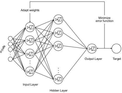
Figure 1.General scheme of an artificial neural network
17
Fig. 1. General scheme of an artificial neural network.
enlarges enormously the fields of application of these artifi-cial neural schemes.
NNs are very helpful systems when numerous examples of the behaviour intended to model are available, since the more examples one has, the simpler the structure of the network can be in order to achieve the same accuracy (Rojas, 1996). It is during the training stage that the NN learns how to model the behaviour/s under study. There are two main types of training: supervised and unsupervised. It is the first one that we have used and whose fundamentals are explained next.
To train the network, a “training set” of patterns is used. For the supervised learning rules, this set is made up of input vectors, each of them with an associated output target (for the unsupervised rules the set consists of inputs only). The components of the input vectors are the values of the “pre-dictors”, or independent variables, and the targets are the val-ues of the “predictand”, or dependent variable, for the corre-sponding input components. For every pattern of the training set, the net releases a certain response, this response is then compared with the corresponding target value, and the error between both quantities is calculated. The error function is then used to adjust the connection weights in order to min-imize the difference between net outputs and targets. There are many different methods of setting the weights (“training algorithms”). We have chosen the Levenberg-Marquardt al-gorithm (Hagan and Mohammad, 1994), which, with respect to the more extended backpropagation algorithm, is faster and more reliable (see next section).
Like what happens in our brains, new interconnections can be established if the learning process requires it (due for ex-ample to the fact that a certain behaviour is observed more frequently). Once the NN has been trained, a set of predic-tors with unknown values for the dependent variable, can be presented to the NN, and then the responses given by the network are expected to have an accuracy within the range reached during the training process. The precision that the system must be able to achieve is one of the parameters that can be modified by the designer, taking into account certain
rules regarding number of patterns and size of the network. 1.2 Advantages for geophysics
Neural networks present several characteristics that make them ideal systems for dealing with atmospheric and cli-matological data. First of all, NNs are non linear systems, which makes them an ideal tool for catching non-linearities. Secondly, they are highly versatile systems which can easily adapt to circumstances, making them able to pick up tem-poral variations, while classical statistics assume the station-arity of the series. NNs are a very useful phenomenologi-cal approach when the dynamics of the problem is either not known or is too complex. In addition, because of the high interconnectivity that a NN presents, this kind of model is very tolerant to errors or noise in the input data. Therefore, NNs are robust and flexible systems which are able to deal with non-linear and non-stationary series. To ensure a better tracking of time variations in the relationships between vari-ables, different strategies can be followed: moving window training set, bootstrapping techniques, ...
In our case we have applied NNs models for the treatment of TO time series. As for almost every climate or weather time series, we have a long available record of data, and we have to deal with extremely non-linear relationships. Solar activity, the chemical composition of the atmosphere, wind regime, or stratospheric intrusions are some of the highly non-linear processes that affect the total amount of ozone. In addition, since the relationships between variables are ex-pected to vary over time, we were interested in a method which is not only able to cope with non-linearities, but also able to track time-changing situations. These reasons led us to consider NNs as the best potential candidate to solve the problem.
Besides, one major advantage of neural nets is that no spe-cial requirements need to be fulfilled a priori by the time se-ries. In general the more complex the problem, the larger the number of data required, but also the size and architecture of the network play a fundamental role. There is no fixed crite-ria to say that the ideal length of the time series should be one or another, simply because there is no fixed criteria to use one type of neural network or another, nor one training algorithm or another. Neural networks are flexible enough to be ap-plied to any time series, provided that some points are taken into consideration. Primarily, the overtraining of the network must be always avoided. Overtraining means that the net is not able to generalize any rules for patterns different from those used for training because it has learned (memorized) the patterns in the training set during the learning stage.
B. M. Monge Sanz and N. J. Medrano Marqu´es: Total ozone time series analysis 685 reach. In our applications this rule has been taken into
ac-count to minimise the risk of having an overfitted network. The next section offers a brief presentation of the data and the methodology we have used, including the NNs configura-tions and the chosen training algorithm. In Sect. 3, one model based on neural networks is presented for the substitution of missing values within the data series and compared with clas-sical statistical techniques. Section 4 deals with time series reconstruction.
2 Data and method
For this work we have chosen TO series corresponding to stations located at European mid-latitudes, which, because of their geographical position, are strongly influenced by atmospheric dynamics. All TO data have been retrieved from the World Ozone and Ultraviolet Radiation Data Centre (WOUDC). The time series used are made up of total ozone mean monthly values for the following locations (Fig. 2): Lisbon (38.8◦N, 9.1◦W) in Portugal, Arosa (46.8◦N, 9.7◦E) in Switzerland, and Vigna di Valle (42.18◦N, 12.2◦E) in Italy.
The artificial NNs we have employed are feedforward con-figurations of the multilayer perceptron (MLP) implemented with Matlab software. Feedforward networks are nets in which signals flow from the input to the output neurons, in a forward direction. There also exist recurrent or feedback networks which have closed-loop paths, from a unit back to itself or to units from a previous layer (Fausset, 1994). Feed-forward networks have been proved to be able to approxi-mate a function with a finite number of discontinuities to any degree of accuracy (Principe et al., 2000).
One of the most extended training algorithms for MLP structures is backpropagation (Rumelhart et al., 1986). This method basically consists of a gradient descent technique based on the Widrow-Hoff rule. However, the algorithm cho-sen to train our ANN models was the Levenberg-Marquardt algorithm (L-M) because, for moderate seized networks, it presents important advantages that help to overcome two of the main problems that arise from backpropagation training: the Levenberg-Marquardt can converge more rapidly, and the risk of the final weights becoming trapped in a local mini-mum is much lower. On the other hand, the L-M algorithm requires more computational memory (Matlab, 1997), since it assesses second derivatives.
Concrete applications of these neural network configura-tions to ozone data series and the results obtained will be discussed next.
3 NNs models for missing data treatment
When dealing with time series, some kind of treatment for the missing data is essential since most of the analysis meth-ods cannot be performed otherwise. Classical methmeth-ods such as substitution of the gaps by the mean value of the series, or
Figure 2. Map of the stations whose data series have been analysed.
18
Fig. 2. Map of the stations whose data series have been analysed.
interpolation from the nearest neighbours, persistence tech-niques or arbitrary value substitution, are unable to catch time variations, or dependence with other variables varia-tions. We propose here the alternative method of using non-linear neural networks to improve missing values substitu-tion.
In order to design the most appropriate network model and training strategy we have distinguished between isolated missing values or long gaps within the data series. In this work we describe how the isolated data within TO series have been filled by using a NN model, and compare the results with those obtained by applying a linear interpolation tech-nique.
For the estimation of the isolated gaps within the data se-ries, thenprevious and thenfollowing values to the missing one are presented as inputs to the network. And then the net releases the searched value. The structure of the network used for this interpolation model is a pyramidal (2n2n-1 1) configuration. For the single output neuron the lineal transfer function is used, while for the other layers the log-sigmoid function has been chosen. Data series were standardized be-fore being processed by the net.
686 B. M. Monge Sanz and N. J. Medrano Marqu´es: Total ozone time series analysis
Table 1. RMSE values for the results obtained with the non-linear
model based on neural networks and with the lineal model, for the three considered data series.
NN non-linear model Linear model station RMSE RMSE Lisbon 0.79 7.62 Vigna di Valle 2.64 3.23 Arosa 2.89 2.99
anomalies.
To evaluate the model performance, simple statistical tests have been applied: the Root-Mean-Square-Error (RMSE) and the explained variance (EV); which also permit an easy comparison with the results obtained with other methods. In our case, the response given by the NN model has been com-pared to the one achieved using a linear interpolation tech-nique. By using a perceptron with linear activation function that has been trained with the LMS method or Widrow-Hoff rule, it is possible to implement a linear interpolation func-tion by way of a simple NN model. This model generates the same results as a linear regression (Widrow and Winter, 1988; Trigo and Palutikof, 1999).
The series of Lisbon for the period June 1967–July 1975 is shown in Fig. 3a. The first part of the dataset, i.e. June 1967–November 1973, was used to train the network, while the set December 1973–July 1975 has been used to validate the model. The validation period is indicated by an arrow. In the graph, the real values are represented by stars and the circles stand for the values released by our NNs based model. The second diagram (Fig. 3b) is the result for the same series and the same period of time but using a linear interpolation model. It can be seen that the performance of the first model is much better: stars and circles match up better for the non-linear model. In fact, the RMSE for the NN non-non-linear model is 0.79% whereas for the linear model it is 7.62%. Results for all the three stations are summarized in Table 1. It is shown that the NN non-linear model improves the results obtained with a linear regression model.
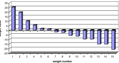
In order to provide further proof of the non-linearity of the model, we include a histogram with the distribution of the weights values for the input layer and the hidden layer (Fig. 4) of the network used in this application. The meaning of the weights in a neural system is not directly comparable with the coefficients in a classical regression model, never-theless, as can be seen from the chart, most of the weights have an absolute value higher than 5, with several above 20. Such a weights distribution points out that the network works far from the linear range of the sigmoidal activation function, so that we can assure that the nonlinear part of the network plays the main role in the model, and that the model we are dealing with is clearly non linear.
In this section the substitution of isolated missing values has been analysed. The estimation of longer gaps requires
Jun67 Jan69 Sep70 Apr72 Jan74 Jul75
-2 -1.5 -1 -0.5 0 0.5 1 1.5 2
Jun67 Jan69 Sep70 Apr72 Jan74 Jul75
-2 -1.5 -1 -0.5 0 0.5 1 1.5 2
(a) non-linear model
(b) linear model
normalized O
3
normalized
O3
Figure 3. Real values (∗) and modelled values (o) for the ozone series of Lisbon during the period Jun67-Jul75. Results for the interval Dec73-Jul75 have been obtained with a non-linear model based on neural networks (a), and with a linear regression model (b). The better performance of the NNs model can be seen.
19
Fig. 3. Real values (∗) and modelled values (o) for the ozone se-ries of Lisbon during the period June 1967–July 1975. Results for the interval December 1973–July 1975 have been obtained with a non-linear model based on neural networks (a), and with a linear regression model (b). The better performance of the NNs model can be seen.
more complex and specific methods, therefore NNs are also a promising alternative to accomplish the task. In Monge-Sanz and Medrano-Marqu´es (2003), non-linear models based on NNs that use the North Atlantic Oscillation Index as a predictor have been successfully applied for the assessment of long missing periods of data.
4 NNs for time series reconstruction
pre-B. M. Monge Sanz and N. J. Medrano Marqu´es: Total ozone time series analysis 687
igure 4. Weights distribution of the neural network used for the interpolation of isolated issing data. The values shown correspond to the input layer and to the hidden layer of the
-25 -20 -15 -10 -5 0 5 10 15 20 25 30
weight value
1 2 3 4 5 6 7 8 9 10 11 12 13 14 15 weight number
F m
net. Since most of them are high values, the network is acting far from the linear range of the sigmoidal function.
20
Fig. 4. Weights distribution of the neural network used for the
in-terpolation of isolated missing data. The values shown correspond to the input layer and to the hidden layer of the net. Since most of them are high values, the network is acting far from the linear range of the sigmoidal function.
dictor because of the high correlation that it presents with the Italian one, and because it is the longest European total ozone record, with observations in this alpine location dat-ing back to the 1920’s. Moreover, the time series of Arosa is not only the longest but also one of the best quality registers of TO because of the revisions and updates that have been made to ensure adaptation between different instrumentation and measurement strategies to provide a homogeneous series (Staehelin et al., 1998). The length and quality of the Arosa register make it the ideal series to predict values for shorter or more incomplete series which are correlated enough.
To find the TO value at Vigna for a certain month, which we call the current month, we use the following set of predic-tors: the n previous values to the considered month of the Vi-gna seires, the n previous of the Arosa series, and the current month value of Arosa. From these inputs the net provides the mean value of TO for the current month at Vigna. For the case analysed here the set of data is June 1967–October 1980, and the period November 1975–October 1980 has been reserved for validation.
The model structure used consists of a two layer MLP with kinput neurons and one cell at the output layer. These mod-els (k+1 models) have been used before for different meteo-rological applications, see for instance (Trigo and Palutikof, 1999); with these models better results are achieved for our application than with more complex structures. For the out-put layer the linear transfer function has been chosen, whilst the quality of the results seems to be independent from the election of the log-sigmoid or the hyperbolic tangent transfer function for the input layer.
For this particular application we have experimented with a technique that is of high interest at the moment because it improves the performance of individual neural networks: as the final signal of our model, we have considered the aver-age of the output of severalk+1 nets. Since we average the results given by several of these k+1 individual networks, the parameter beingk=1,. . . , 2n+1 (onekvalue for one net-work), we are using a “neural network ensemble”. The neu-ral network ensembles technique is a learning scheme where
-2.0 -1.5 -1.0 -0.5 0.0 0.5 1.0 1.5 2.0 2.5
nov-75 mar-76 jul-76 nov-76 mar-77 jul-77 nov-77 mar-78 jul-78 nov-78 mar-79 jul-79 nov-79 mar-80 jul-80
normalized ozone
Figure 5. One month ahead reconstruction for Vigna di Valle by way of the NNs ensemble
k+1 for n=1 (red line), and the observed real series at the station from November 1975 to
October 1980 (black line).
21
Fig. 5. One month ahead reconstruction for Vigna di Valle by way
of the NNs ensemblek+1 forn=1 (red line), and the observed real series at the station from November 1975 to October 1980 (black line).
a finite number of individual networks is trained to solve a problem.
A neural network ensemble consists of a set of different individual neural networks, trained with the same or different predictors, in order to give the same output variable. The output of the ensemble is a combination of the outputs of the individual NNs. It has been shown that the generalization capability of a NN can be improved by using this kind of ensemble learning (Sharkey, 1999). The way the individual predictions are combined strongly depends on the application the ensemble is used for. For regression tasks, as is our case, the individual outputs can be averaged (Opitz and Shavlik 1996) or weight averaged (Perrone and Cooper 1993); while for classification majority voting may be an ideal combining approach (Hansen and Salamon, 1990).
The ensemble we have used is made up of a collection of neural networks, each of these networks with a different numberk of input cells. For a given number n of values of the Vigna series, the ensemble contains 2n+1 networks, every network with its correspondingk, and the parameterk takes values from 1 to 2n+1. In our application, every net in the ensemble provides the mean value of TO. By taking the average of all these responses (output of the ensemble) as the final signal of our model, we get an answer with a lower variance.
The method of the neural network ensembles has however a substantial drawback: ensembles are more difficult to inter-pret than single networks, although some works have already addressed the problem of the extraction of rules from these structures, see for instance (Zhou et al., 2003).
In Fig. 5 the results obtained with the model k=1, and withn=1, are represented together with the real signal for the time interval under consideration. The high explained vari-ance value (EV>88.0%) means that the shape of the original signal is accurately reproduced by the model.
recon-688 B. M. Monge Sanz and N. J. Medrano Marqu´es: Total ozone time series analysis
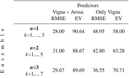
Table 2. RMSE and EV values for the forward reconstruction of
Vi-gna series, comparing the inclusion of Arosa data as an input vari-able with the results obtained using the Vigna series only.
E
n
s
e
m
b
l
e
Predictors
Vigna + Arosa Only Vigna RMSE EV RMSE EV
n=1
k=1, ..., 3 28.00 90.64 48.95 58.00
n=2
k=1,.., 5 31.00 88.67 42.80 63.28
n=3
k=1,.., 7 29.67 89.69 36.55 70.71 All numerical values in this table are percentage values.
struction of the Vigna series is tried using only data from this series, and the results attained with the inclusion of Arosa data in the model.
As can be deduced from Table 2, better results are ob-tained when Arosa is included as a predictor, lower RMSE and higher correlation are achieved. In addition, the spread in the RMSE and EV values is a good indicator for the ro-bustness of the strategy: when we use only Vigna the results seem to be much more dependent on the number of inputs and the particular ensemble used.
In general, the inclusion of related variables as predictors for the model will always improve the quality of the results. Although it is true that one must consider whether such in-clusions offer a sufficiently worthwhile improvement for the computational cost they imply. In cases like ours, where both the size of the network and the number of input variables are rather small, the benefits of including a second variable, here Arosa series, compensate by far for the minimal increase in the computing time of the model, which still remains within the order of 10 s.
Besides, we are passing from having just one predictor se-ries (Vigna) to having two predictor sese-ries (Arosa and Vi-gna), in a case like this, with any kind of model, not just with neural network schemes, one must expect more benefits than problems.
Considering again the results in Fig. 5, one can state that, given the high correlation between real and modelled series and the ability of this NNs structure to predict the right sign of the TO variations, it is shown that the model including Arosa, without any modification, is suitable for forecasting the sign of TO monthly anomalies. However, if we want to improve accuracy for the exact values we should include new predictors, such as for example the Arctic Oscillation Index, which exhibits very high correlations with TO series throughout the whole year over these European areas (Stae-helin et al., 2002; Monge-Sanz et al., 2003).
5 Future work and concluding remarks
Because of their great versatility and capability of dealing with non-linear and non stationary series, neural network systems are the ideal approach for geoscience data treatment. In this work, several models based on NNs for the analysis of TO time series have been presented for different appli-cations concerning missing data treatment and time series reconstruction. Such models have proved to achieve better results than some other classical techniques. In addition, the simplicity of our NNs based models allows us to consider further applications without the risk of involving schemes which are too complex or time consuming. Some of these ap-plications involve the backwards-reconstruction of time se-ries into pre-instrumental periods, or the forecasting of the magnitude under analysis. Different time-scales can also be considered just by choosing the appropriate set of predictors.
Acknowledgements. The authors are grateful to the World Ozone
and Ultraviolet Radiation Data Centre (WOUDC) for providing ozone data, and to the Climatic Research Unit (CRU) of the University of East Anglia for the NAO Index data series. Our special thanks go to A. F. Pacheco for his continuous support and advice during the realization of this work, and his encouragement to develop it further. We also thank the anonymous referees for their constructive remarks and suggestions which have greatly helped to improve the quality of this paper.
Edited by: M. Thiel Reviwed by: two referees
References
Acciani, G., D’Orazio, A., Delmedico, V., De Sario, M., Gramegna, T., Petruzzelli, V. and Prudenzano, F.: Radiometric profiling of temperature using algorithm based on neural networks, Electron. Lett., 39, 17, 1261–1263, 2003.
Alsayegh, O. A.: Short-term load forecasting using seasonal artifi-cial neural networks, In. J. Power Energy Sys., 23, 3, 137–142, 2003.
Baum, E. B.: A proposal for more powerful learning algorithms, Neural Computation, 1, 295–311, 1989.
Chevallier, F., Morcrette, J.-J., Cheruy, F., and Scott, N. A.: Use of a neural-network-based longwave radiative transfer scheme in the ECMWF atmospheric model, Quart. J. Roy. Meteor. Soc., 126, 761–776, 2000.
Fausset, L.: Fundamentals of Neural Networks. Architectures, Al-gorithms and Applications, Prentice Hall International Editions, New Jersey, 1994.
Hagan, M. and Mohammad, B.: Training Feedforward Networks with the Marquardt Algorithm, IEEE Transactions on Neural Networks, 5, 6, 989–993, 1994.
Hansen, L. K. and Salamon, P.: Neural network ensembles, IEEE Transactions on Pattern Analysis and Machine Intelligence, 12, 993–1001, 1990.
Haykin, S.: Neural networks, A comprehensive foundation, 2nd edition, Prentice-Hall, 1999.
of Circuits and Integrated Systems, DCIS 2003, Ciudad Real (Spain), 2003.
Mac´ıas Mac´ıas, M., L´opez Aligu´e, F., Serrano P´erez, A., and Astilleros Vivas, A.: A comparative study of two neural models for cloud screening of Iberian Peninsula Meteosat images, edited by Mira, J., Springer Verlag, Berlin Heidelberg, IWANN 2001, LNCS 2085, 184–191, 2001.
Mart´ın del Br´ıo, B., Medrano, N., Ram´ırez, I., Dom´ınguez, J.A., Barquillas, J., Blasco, J., and Garc´ıa, J.: Short-term electric power load forecasting using artificial neural networks. Part I: self-organizing networks for classification of day-types, 14th IASTED Int. Conf. On Modelling, Identification and Control, Igsl, Austria, 1995.
Mart´ın del Br´ıo, B. and Serrano Cinca, C.: Self-organizing neural networks for an´alisis and representions of data: Some financial cases, Neural Computing and Applications, 1, 193–206, 1993. MATLAB Reference Guide: Neural Networks Toolbox User’s
Guide, 1997.
Medrano, N. and Mart´ın del Br´ıo, B.: Computer voice interface us-ing the mouse port, XVI Design of Integrated Circuits and Sys-tems Conference, DCIS 2000, Montpellier, France, 2000. Mitchell, T.: Machine Learning, McGraw Hill, 1997.
Monge-Sanz, B. and Medrano Marqu´es, N.: Artificial Neural Net-works Applications for Total Ozone Time Series, edited by Miram, J., Springer Verlag, Berlin Heidelberg, IWANN 2003, LNCS 2687, 806–813, 2003.
Monge-Sanz, B. M., Casale, G. R., Palmieri, S., and Siani, A. M.: Ozone Loss over South Western Europe, Its Relation with Circu-lation and Transport, Air Pollution Research Report 79, Strato-spheric Ozone 2002, European Commission, Belgium, 396–399, 2003.
M¨uller, M. D., Kaifel, A. K., Weber, M., and Tellmann, S.: Real-time total ozone and ozone profiles retrieved from GOME data using neural networks, in Proceedings 2001 EUMETSAT mete-orological Satellite Data User’s Conference, Antalya, EUMET-SAT, Darmstadt, Germany, 2001.
Olsson, J., Uvo, C. B., Jinno, K., Kawamura, A., Nishiyama, K., Koreeda, N., Nakashima, T., and Morita, O.: Neural Networks for Rainfall Forecasting by Atmospheric Downscaling, J. Hydr. Engin., 9, 1, 1–12, 2004.
Opitz, D. W. and Shavlik, J. W.: Actively searching for an effec-tive neural network ensemble, Connection Science, 8, 337–353, 1996.
Perrone M. P. and Cooper, L. N.: When networks disagree: Ensem-ble method for neural networks. Artificial Neural Networks for Speech and Vision, edited by Mammone, R. J., Chapman & Hall, New York, 126–142, 1993.
Principe, J., Euliano, N., and Lefebvre, W.: Neural and Adaptive Systems, Wiley, 2000.
Reusch, D. B. and Alley, R. B.: Automatic weather stations and artificial neural networks: improving the instrumental record in West Antarctica, Monthly Weather Review, 130, 12, 3037–3053, 2002.
Rojas, R.: Neural Networks, a Systematic Introduction, Springer-Verlag, 1996.
Rumelhart, D. E., Hinton, G. E., and McClelland, J. L.: A Gen-eral Framework for Parallel distributed Processing, Parallel Dis-tributed Processing, edited by Rumelhart, D. E. and McClelland, J. L., Foundations, 1, 1986.
Sharkey, A. J. C.: Combining Artificial Neural Nets: Ensemble and Modular Multi-Net Systems, Springer-Verlag, 1999.
Staehelin, J., M¨ader, J., Weiss, A. K., and Appenzeller, C.: Long-term ozone trends in Northern mid-latitudes with special em-phasis on the contribution of changes in dynamics, Phys. Chem. Earth, 27, 461–469, 2002.
Staehelin, J., Renaud, A., Bader, J., McPeters, R., Viatte, P., Hoeg-ger, B., Bugnion, V., Giroud, M., and Schill, H.: Total ozone series at Arosa (Switzerland): Homogeneization and data com-parison. J. Geophys. Res., 103, D5, 5827–5841, 1998.
Trigo, R. M. and Palutikof, J. P.: Simulation of daily temperatures for climate change scenarios over Portugal: a neural network ap-proach, Climate Res., 13, 45–59, 1999.
Vega-Corona, A., ´Alvarez-Vellisco, A., and Andina, D.: Feature vectors generation for detection of microcalcifications in digi-tized mammography using neural networks, edited by Mira, J., Springer Verlag, Berlin Heidelberg, IWANN 2003, LNCS 2687, 583–590, 2003.
Widrow, B. and Winter, R.: Neural nets for adaptive filtering and adaptive pattern recognition, IEEE Computer, 1988.