Hybrid Simulation Using SAHISim Framework

(1)

Hybrid Simulation Using SAHISim Framework

[A Hybrid Distributed Simulation Framework Using Waveform Relaxation Method

Implemented Over the HLA and the Functional Mock-up Interface]

Muhammad Usman

Awais

Austrian Institute of Technology Giefinggasse 2 1210 Vienna, Austria

Muhammad.Awais.fl

@ait.ac.at

Wolfgang Gawlik

Vienna University of

Technology

Gusshausstrasse 25/370-1 1040 Vienna, Austria

wolfgang.gawlik

@tuwien.ac.at

Gregor De-Cillia

Austrian Institute of

Technology Giefinggasse 2 1210 Vienna, Austria

Gregor.DeCillia.fl

@ait.ac.at

Peter Palensky

Delft University of Technology

Department of Electrical Sustainable Energy

[email protected]

ABSTRACT

Hybrid systems such as Cyber Physical Systems (CPS) are becoming more important with time. Apart from CPS there are many hybrid systems in nature. To perform a simulation based analysis of a hybrid system, a simulation framework is presented, named SAHISim. It is based on the most popular simulation interoperability standards, i.e. High Level Ar-chitecture (HLA) and Functional Mock-up Interface (FMI). Being a distributed architecture it is able to execute on clus-ter, cloud and other distributed topologies. Moreover, as it is based on standards so it allows many different simulation packages to interoperate, making it a flexible and robust solution for simulation based analysis. The underlying al-gorithm which enables the synchronization of different sim-ulation components is discussed in detail. A test example is presented, whose results are compared to a monolithic simulation of the same model for verification of results.

Categories and Subject Descriptors

I.6.0 [Simulation and Modeling]: General

Keywords

High Level Architecture, Functional Mock-up Interface, Mod-elica, OpenModMod-elica, Simulation Interoperability, Hybrid Sim-ulation, Co-simSim-ulation, Heterogeneous Simulation

1. INTRODUCTION

Standardized Architecture for Hybrid Interoperability of Sim-ulations (SAHISim) is a newly proposed framework. It sup-ports distributed simulation by conforming to High Level Architecture (HLA) [7]. It is flexible and robust; because individual federates can be FMI [2] components (Functional Mock-up Units (FMUs)). The purpose of developing SAHISim is to provide simulation engineers a platform which

• Supports interoperability among different simulation packages.

• Is able to add parallelism through distribution

• Supports hybrid simulation

Simulation interoperabilityis becoming very important in modern research and analysis. Because there are so many specialized simulation packages for different types of sys-tems, it is appealing to use specialized simulation packages for any two or more domains and couple them to analyze results of the system. This saves considerable effort of de-veloping and testing a new simulation package which could cover many domains. This is similar to the re-usability trend humanity has enacted in every other domain.

Interoperability among simulations becomes more vital when it can offer parallelism through distribution. Because simulation is established as a good method of verification, large scale simulations are becoming appealing in industry to verify policies and designs. Large scale simulations re-quire large amount of computing resources. Running large scale simulations on monolithic platforms can result into re-source starvation. By distributing the execution of different subsystems onto different machines, parallel execution can improve the overall performance. It can be used to avoid resource starvation by adding more remote resources.

(2)

Simulation of hybrid systemshas been a major challenge for researchers in the field of modeling and simulation. It has become even more important due to intermix of Infor-mation and Communication Technology (ICT) with other technologies. Due to the discrete aspects of ICT, its cou-pling with any continuous physical system leads to a hybrid system. Interoperability becomes essential in this scenario, because like other domains ICT has its own breed of special-ized simulation packages. Coupling an ICT oriented simula-tion package with a simulasimula-tion package for a physical phe-nomenon requires both interoperability and hybridization of the simulation.

In next section previous approaches to hybrid system sulators are discussed. Then the simulation algorithm im-plemented in SAHISim framework is discussed in detail in section 3. After understanding the underlying working of the framework, results of a test example are presented in section 4, followed by a brief conclusion.

In the presented paper, major focus is on developing a syn-chronization algorithm for hybrid systems. The algorithm, with a little effort, can be adapted to any platform, in that case though, it will lose some functionality. For example, if it is implemented without the HLA then it will lose the ability to create simulation on distributed environments. If something else is placed instead of HLA then it will lose its standardized format. FMUs are the basic simulation com-ponents of the framework. If FMUs are replaced by some other components then again it will lose its standardized format. Nevertheless, the presented algorithm serves well to facilitate a distributed hybrid simulation.

2. RELATED WORK

Due to introduction of ICT into power grids management, it has become vital to simulate power grids in conjunction with ICT infrastructure. In recent past there have been quite a number of efforts to couple ICT network simulators with power system simulators [11] to simulate cyber phys-ical energy systems, or to simulate smart grids [14]. Most smart grid simulators do not try to couple more than one continuous systems. Only a continuous power system sim-ulator is coupled with a discrete network simsim-ulator. In this case the system formed does not have any algebraic rela-tionship among simulation components, which makes things much easier and manageable.

When a simulation has more than one continuous simulators in the federation, things become much more complex. Many real world scenarios require such a simulation. For example, a complex energy system simulation may also need to cou-ple thermal energy simulator along with power and network simulators. In case of more than one continuous simulators, coupling may form a Differential Algebraic Equation (DAE) with index≥1. When such tightly coupled systems are inte-grated over time domain, explicit methods normally do not produce good results [6]. The presented algorithm can deal with any number of continuous or discrete event simulators coupled with each other.

There have been other attempts to orchestrate hybrid sim-ulations (alternatively called as “heterogeneous simulation”) for example, Discrete EVent Specification (DEVS). DEVS

provides a systematic way to convert a continuous simula-tor into a discrete event simulasimula-tor [4]. In this way there is no difference left in coupled continuous or discrete event simulation. Although, there are still some questions related to its stability [3]. The biggest disadvantage of DEVS is its lack of interoperability with other simulation paradigms. In order to orchestrate a DEVS based federation all simulation federates must conform to DEVS specification.

Ptolemy II is another solution which aims to provide hybrid simulation platform. According to some [9] the Ptolemy Discrete Event Model Specification (PDEMS) can be con-sidered equal to DEVS. Ptolemy II is supplemented by sup-port for FMI [12], which makes it more usable in terms of interoperability than DEVS. However, Ptolemy II is mono-lithic in nature and there is still a lot of work to be done to make it distributed in nature. Secondly, there are some underlying restrictions imposed by Ptolemy II kernel which makes it difficult to implement new synchronization algo-rithms in Ptolemy II. Lasnier et al. [8] have used feder-ates implemented using Ptolemy with HLA. They use the Discrete Event (DE) director of Ptolemy for federate imple-mentation, which cannot be better than the discretization technique proposed by DEVS experts.

Techniques like [8] and [13] use nonzero lookahead based tim-ing services of the HLA. They can be considered as explicit and hence less stable [6]. They are explicit, because for a DAE predicting “precisely” when next event will occur is not possible without actually integrating the DAE. In case of a tightly coupled system of DAEs modeled as separate feder-ates, it is impossible to know the exact time of an event of a federate independently. In such a situation the guess work involved in setting the lookahead value and length of time step makes the solution even more erroneous.

3. DESCRIPTION OF THE ALGORITHM

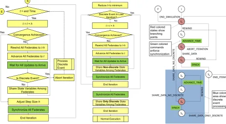
The underlying execution of simulation using SAHISim frame-work is governed by a master-slave algorithm. The master algorithm works like an orchestrator. It directs the slaves to perform some action by sending them commands. The slave algorithm is a state machine, whose states are changed based on the commands received from the master. The ac-tual numerical integration is performed at salve only, but master has to check for convergence. To check convergence, master needs to know the values of state variables at each iteration. Based on the values of state variables, master also changes the step size. Handling of discrete event is also dependent on the master. The slave which experiences a discrete event informs the master about the event, and then master orchestrates the method to handle it.

3.1 The master algorithm

The algorithm shown in figure 1a describes the flow of mas-ter. The master algorithm has only one instance for one simulation federation. There is no limitation on the number of slaves.

(3)

t < end Time

Convergence Achieved?

Rewind All Federates to t-h

No S

E

Yes No

t = t + h

Advance All Federates to t

Wait for All Updates to Arrive

Is Discrete Event? Yes

Share State Variables Among Federates

No

Adjust Step Size h

Yes

Synchronize All Federates

End Iteration

Abort Iteration Process Discrete Event

(a) Main flow of the master algorithm, highlighted in green are steps which en-force all the slaves to get synchronized.

Discrete Event In Last Iteration?

Convergence Achieved?

No No

Yes

t = t + h

Share Non-discrete State Variables Among Federates Yes

Share Only Discrete State Variables Among Federates Reduce h to minimum

Normal Execution End Iteration End Iteration Rewind All Federates to t-h

Advance All Federates to t

Wait for All Updates to Arrive

(b) Discrete event processing. Here h represents the step size, andt represents the time.

I END_SIMULATION

S1

F

S2

REWIND

S3

ADVANCE_TIME

S4

ABORT_ITERATION SHARE_DATA

SH

AR

E_

D

A

TA_NO_DISCR

ETE

REWIND

S5

SYNCH

RE

WIND

S7

ADVANCE_TIME

S9

SHARE_DATA_NO_DISCRETE

SYNCH

SHARE_DATA_ONLY_DISCRETE END_ITERATION

S8

S6

Blue colored area shows discrete event processing Red colored

states show branching points

Green colored commands enforce synchronization

(c) State machine of the slave.

So the algorithm works fine for both hybrid and continuous systems.

3.2 Slave State Machine

The slave works like a state machine. Figure 1c shows that how different commands take slave from one state to an-other. State based execution is essential for a slave to avoid ambiguities. State based execution ensures that a slave will always keep following the correct path. Highlighted in red are the states which have a branching factor greater than 1. From these states a slave may go in wrong direction of execution if there was no method of synchronization.

3.3 Working of Algorithm

The mathematical motivation for the presented algorithm comes from the Waveform Relaxation (WR) algorithm [10]. The WR algorithm is only focused on the continuous simula-tions and does not mention handling of discrete events. The presented work augments the WR algorithm by introducing the logic of handling discrete events. The WR algorithm is based on the idea of Banach spaces, or fixed point iteration [5]. The idea is, if there is a system of Ordinary Differential Equations (ODEs), then if the state based representations of ODEs are separated in a way that performing a WR iter-ation is contractive in nature, then the system of equiter-ations is guaranteed to converge at each time step [10]. From one time step to another WR iteration is performed repeatedly, and at each time step the system converges at a single point, called the fixed point. In order to have a successful separa-tion of ODEs few guideline are mensepara-tioned in the original work [10]. The WR iteration is a very simple phenomenon itself. Figure 2 shows the execution cycle of a WR itera-tion. All the ODE based subsystems are evaluated at time

tn+1. The output of each subsystem is propagated to other

dependent subsystems. The output values of one subsystem become the inputs for others. The time is rewound to tn

and now the state variables of each subsystem are evaluated again attn+1. Continuing in this way, after few iterations

the fixed point is reached, then the same procedure is used fortn+2, tn+3 , so on and so forth. Here tn is termed as a

“communication point”.

Subsystem1

Subsystem2

Internal integration

Tn Tn+1

1.2 1.1

Figure 2: Waveform Re-laxation iteration. In-tegration of one subsys-tem from time Tn to

Tn+1 is completely

inde-pendent. The numeri-cal solver of a subsystem, its internal step size or any other related informa-tion is completely isolated from outer working of the algorithm.

3.4 Explanation of Commands

The slave algorithm only follows the commands, so it is very important to understand their meaning. The actions taken to follow the commands are straight forward. The “REWIND” command takes the FMU back in time. This means that the time and state variables of the FMU are set to the values converged at the end of previous com-munication step. The “ADVANCE TIME” is the command where actual integration of the subsystem (here FMU) is done. The command takes a parameter, which is the “time” to which an FMU should integrate. This is the time tn

(4)

occur for convergence. The “ABORT ITERATION” com-mand is a level stronger than “REWIND” comcom-mand. The “ABORT ITERATION” command not only goes back in terms of time and state variables, but it also reverts to in-puts valid at the end of previous successful communication step.

The “SYNCH” command is just used for the synchronization purpose. On receiving “SYNCH” command a slave sends its time to the master. Immediately after sending “SYNCH” command the master goes into an infinite loop until it re-ceives updates from all the FMUs. It is a subject of detailed discussion how positioning this command correctly ensures correct order of execution. The proof is omitted for the sake of brevity.

The “SHARE DATA” command asks all FMUs to share state variables. The sharing happens with the help of object man-agement services of HLA. As a rule of thumb one state vari-able must be published by only one federate, but it can be subscribed by many.

The working of commands “SHARE DATA NO DISCRETE” and “SHARE DATA ONLY DISCRETE” is just the same as “SHARE DATA”, but there are semantic differences. Both of these commands are only used when processing a dis-crete event. The “SHARE DATA NO DISCRETE” initiates a change in the slave state machine. On receiving this com-mand it is known that there is a discrete event processing going on. It asks salves to share all states except the discrete ones. The “SHARE DATA ONLY DISCRETE’ command is executed only once in an iteration. In result the internal behavioral change necessary to occur due to a discrete event is accomplished at once.

The command “END ITERATION” is issued when the con-vergence is achieved for one communication step. On receiv-ing this command an FMU closes the internal integration step and prepares for the next communication step.

3.5 Processing Discrete Event

First of all, this should be kept in mind that before pro-cessing the discrete event the iteration where the discrete event was detected has already been aborted. Abortion of the iteration means that all the FMUs go back to the state (including input variables) where they were at the end of the last communication step. The easiest way to process the discrete event is to reduce the step size to minimum and keep on progressing the simulation. Decreasing the step size to minimum ascertains that the precise time of event cannot be missed by far, which reduces the chances of error prop-agation. The simulation with minimum step size continues until the discrete event has occurred again. After the it-eration in which discrete event occurs, the master switches back to the normal mode of execution.

3.6 HLA Timing Services

Time Advance Request (TAR) and Time Advance Request Available (TARA) services are used in collaboration at both master and slave level. The step size is calculated by the master at the end of each communication point. Before con-vergence TARA service is used repeatedly by the master and the slaves, to get the updates. Once the convergence is

achieved and “END ITERATION” command is issued, the TAR service is invoked by the master and slaves to close the episode. In this way any discrete event simulator using the same services will not have any problem in co-simulation.

For clarity it is important to mention that when a feder-ate issues TARA request with time t0 then it announces

that it may send more updates at the same timet0.

Sim-ilarly, it is ready to accept more updates from other feder-ates att0. Once the master decides that it is done with the

iteration and there are no more updates needed, it issues “END ITERATION” command with TAR at timet0,

sub-sequently all slaves also issue TAR. After issuing TAR any federate can send an update only at a time t0+for any

>0.

3.7 Communication Step Size Control

Step size control offers many advantages in any numerical integration algorithm. Implemented correctly, it can signifi-cantly enhance the performance of the algorithm. Here too, the communication step size control offers many advantages. Most importantly, in a distributed simulation more com-munication steps mean more comcom-munication, which means lesser performance. So increasing the communication step size to the maximum where the solution remains valid is very beneficial.

Looking at the figure 2, it is easy to understand that separat-ing the ODEs means that some or all of the sate variables in subsystems are going to grow independent of partial deriva-tives of each other. Mathematically speaking, suppose there is a system given in equation 1

˙

y=f(y, p) (1)

The state vector y contains n state variables y = y1, y2, y3, . . . , yn. To perform the numerical

integra-tion of the system, if an implicit method is used, then the Jacobian of the system will be n×n matrix, containing partial derivatives of all the state variables with respect to each of them. Partitioning the system in two (equation 2) means that the Jacobian of each subsystem is also re-duced to some degree. If ˆy = y1, y2, y3, . . . , yi and ˜y =

yi+1, yi+2, yi+3, . . . , yn, then this means that state variables

in ˆy are being evaluated without their partial derivatives with respect to yi+1, yi+2, yi+3, . . . , yn. Similar is the case

of ˜y. This causes divergence in the solution. If the diver-gence remains in the realm where the system remains defined then it is possible to recover the error through fixed point iteration. If not, then this means that the gap between two communication steps is too large.

˙ˆ

y= ˆf(ˆy,pˆ) ˙˜

y= ˜f(˜y,p˜) (2)

Following the idea of divergence, apart from error tolerance, there is an additional parameter introduced, which is called as “divergence tolerance”told. This is tolerance for the error

caused by divergence. If the state variable vector, as a result of initial guess at the start of WR iteration, isyi, and at the

end of WR iteration after convergence isyf, then the error

edcaused by divergence is given in equation 3.

(5)

8,98 9 9,02 9,04 9,06 9,08 9,1 9,12

1,31 1,315 1,32 1,325 1,33 1,335 1,34 1,345 1,35 1,355 1,36

Y

Time

Figure 3: Variation of communication step size during pro-cessing of discrete event.

At the end of each WR iteration the communication step size is either increased or decreased by some percent, based on the fact that ed + τ0kyf − yikmax < told or

ed+τ0kyf−yikmax> told. Hereτ0 is a small positive value

used for normalization. As mentioned in section 3.5, during processing of discrete event, the communication step size is intermediately reduced to minimum. After the discrete event, communication step size takes some time to recover its value. At that moment the mechanics of communica-tion step size control become evident. Figure 3 shows the phenomenon by zooming into that situation.

4. TEST CASE

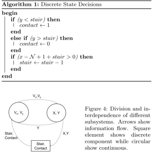
To check the correctness of algorithm a test system is used for simulation. It is first simulated using the OpenModel-ica1. The results are compared with the SAHISim algorithm presented earlier. The system is very popular hybrid system i.e. a ball being dropped from a height on stairs, namely a “bouncing ball on stairs”. The system is given by the system

of equations 4. The discrete part is given by algorithm 1

˙ x=vx

˙ y=vy

˙

vx=−c0vx

˙

vy=−g−c1vy−contact((y−stair)c2+c3vy)

(4)

Heregis the gravitational constant, while c0,c1,c2 andc3

are few constants facilitating the phenomena of friction, air resistance, damping and mass of the ball. The variables stairandcontactrepresent discrete variables. The variable contact shows that the ball is in contact with the floor or not. Whencontact= 1 the system shifts its behavior imme-diately at that point. This is what is called as “behavioral state change”. The variablestairshows that on which step of the stair ball is currently bouncing. Initially, its value is

N used in algorithm 1.

Figure 4 shows how different FMUs are associated to each other, via their state variables. All the subsystems are in form of FMUs, which shows the ability of SAHISim frame-work to generically host any simulation comprising of com-ponents conforming to FMI. Figure 5 shows the simula-tion results of all continuous state variables, as simulated

1

https://www.openmodelica.org/

Algorithm 1:Discrete State Decisions

begin

if (y < stair)then contact←1 end

else if(y > stair)then contact←0

end

if (x− N + 1 +stair >0)then stair←stair−1

end end

Vx, Vy X, Y

Stair, Contact Vx,Vy

Y

X,Y Stair,

Contact

Figure 4: Division and in-terdependence of different subsystems. Arrows show information flow. Square element shows discrete component while circular show continuous.

by OpenModelica. The results of SAHISim simulation are shown in figures 5. It is clear that the over all behaviors of both systems are similar, with little differences.

For the presented run, the value of “divergence tolerance” wastold= 1×10−3. Although, the value is relatively large,

using a smaller value makes results more accurate, but that causes more communication steps and hence performance deteriorates.

5. CONCLUSION

The paper presents Standardized Architecture for Hybrid Interoperability of Simulations (SAHISim). In depth dis-cussion on the working of synchronization algorithm and data sharing using HLA services is presented. The use of SAHISim framework is very easy, it abstracts away tedious configuration details of HLA and makes it very easy for the user to orchestrate a federated simulation. A generic thin layer is implemented to enable the use of FMUs as feder-ates of the simulation federation. Enabling FMI makes the solution very flexible because there are more than forty sim-ulation packages2 _{either supporting or planning to support}

FMI. Currently only FMI 1.0 compliant components are sup-ported by SAHISim. The main reason is that FMI 2.0 is not yet supported by open source simulation packages.

The algorithm used by SAHISim is discussed in detail. The use of presented algorithm is not tied to the use of SAHISim. It can be used in many different ways, independent of SAHISim framework. A test example comparing the results with a monolithic simulation package (OpenModelica) shows the correctness of the results. The results are promising and in-spire further development. There are few problems still to be tackled. Currently, individual subsystems are integrated using self-developed solvers. In order to use industry level solvers it is important to make few changes in them. The

2

(6)

0 1 2 3 4 5 6 7 8 9 10 11 12

0 5 10 15 20 25 30 35 40 45 50 55

x y

Time

0 1 2 3 4 5 6 7 8 9 10 11 12

0 5 10 15 20 25 30 35 40 45 50 55

x y

Time

4 5 6 7 8 9 10 11

0 1 2 3 4 5 6

X Y

4 5 6 7 8 9 10 11

0 1 2 3 4 5 6

X Y

Figure 5: On left the results from SAHISim are shown, on right are the results obtained from OpenModelica.

most important change is to be able to rewind the solver to the previously calculated state. If professional solvers can incorporate this change, then it will enable their use in SAHISim framework, making it even more robust.

6. REFERENCES

[1] M. Awais, P. Palensky, A. Elsheikh, E. Widl, and M. Stifter. The high level architecture RTI as a master to the functional mock-up interface components. In

International Workshop on Cyber-Physical System (CPS) and its Computing and Networking Design (ICNC 2013), pages 315–320, January 2013. [2] T. Blochwitz, M. Otter, M. Arnold, C. Bausch,

C. Clauß, et al. The functional mockup interface for tool independent exchange of simulation models. In

Modelica’2011 Conference, pages 20–22, March 2011. [3] F. E. Cellier and E. Kofman.Continuous system

simulation. Springer US, 2006.

[4] M. D’Abreu and G. Wainer. Models for continuous and hybrid system simulation. InSimulation Conference, 2003. Proceedings of the 2003 Winter, volume 1, pages 641–649 Vol.1, Dec 2003.

[5] V. Istrc et al.Fixed point theory: an introduction, volume 7 ofMathematics and Its Applications. Springer, 1981.

[6] R. K¨ubler and W. Schiehlen. Two methods of simulator coupling.Mathematical and Computer Modelling of Dynamical Systems, 6(2):93–113, 2000. [7] F. Kuhl, R. Weatherly, and J. Dahmann.Creating

computer simulation systems: an introduction to the high level architecture. Prentice Hall PTR, 1999. [8] G. Lasnier, J. Cardoso, P. Siron, C. Pagetti, and

P. Derler. Distributed simulation of heterogeneous and real-time systems. InProceedings of the 2013

IEEE/ACM 17th International Symposium on Distributed Simulation and Real Time Applications, pages 55–62. IEEE Computer Society, 2013.

[9] H. Y. Lee, W.-T. Kim, I.-G. Chun, W. Kang, and S.-M. Park. A formal representation of discrete event models in ptolemy ii. InAdvanced Communication Technology (ICACT), 2010 The 12th International Conference on, volume 1, pages 864–869, Feb 2010. [10] E. Lelarasmee, A. E. Ruehli, and A. L.

Sangiovanni-Vincentelli. The waveform relaxation method for time-domain analysis of large scale integrated circuits.IEEE Transactions on Computer-Aided Design of Integrated Circuits and Systems, 1(3):131–145, 1982.

[11] K. Mets, J. Ojea, and C. Develder. Combining power and communication network simulation for

cost-effective smart grid analysis.Communications Surveys & Tutorials,, Issue: 99:xx, 2014.

[12] W. M¨uller and E. Widl. Linking FMI-based components with discrete event systems. In2013 IEEE International Systems Conference Proceedings, page 5 pages. IEEE Conference Publications, 2013. [13] H. Neema, J. Gohl, Z. Lattmann, J. Sztipanovits,

G. Karsai, S. Neema, T. Bapty, J. Batteh,

H. Tummescheit, and C. Sureshkumar. Model-based integration platform for fmi co-simulation and heterogeneous simulations of cyber-physical systems. In10th International Modelica Conference, pages 10–12, 2014.