Determining Slope Stability by Rigid Finite Element Method and Limit Analysis Methods

(1)

Determining Slope Stability by Rigid Finite

Element Method and Limit Analysis Methods

AmirMohammad Merati

1*

_{, Hasan Ghasemzadeh}

2

_{and Seyyed MohammadFarid}

Astaneh

3

1- MSc in Soil Mechanics & foundation

2- Associate prof. at K.N.Toosi University of Technology 3- Assistant prof. at Islamic Azad University, Central Tehran Branch

Corresponding author

:

AmirMohammad Merati

ABSTRACT: The analysis of soil slopes stability is an issue being analyzed using various methods such as limit equilibrium and its relevant software. In this paper, limit equilibrium method based on plasticity theory has been used. In this paper, Based on upper and lower bound limit theorem and using principle of virtual work for calculations, the authors will introduce an overturning failure criterion to govern both the kinematically and statically admissible ﬁelds in the limit analysis and overall factor of safety of slopes stability is introduced at the end of this research. This research utilizes rigid finite element method considering the rotating-sliding mechanism. The results comparisons of the current research with previous ones show considerable results.

Keywords: Slope stability, Limit analysis, Plasticity, Rigid finite element method, Linear programming. INTRODUCTION

The Finite Element Method (FEM) based on limit analysis is a conventional method in analyzing the limit state issues for various researchers. An obvious drawback with the traditional FEM-based limit analysis approaches being applied to rock slopes is their inability to characterize the behavior of discontinuous rock masses. In this regard, a good alternative would be the rigid FEM. REFM is inspired by a technique called Rigid Body Spring Model (RFSM) introduced in 1977. (1)

With a lower degree of freedom for the elements considered in the RFEM than that in the traditional FEM, the computational efﬁciency may be much improved. Importantly, the physical discontinuities in discontinuous media can be reasonably treated as interfaces between the adjacent rigid elements in RFEM. (2)

In RFEM, The pre-process of data and the process of analysis is same as conventional FEM but the difference is that the main 2 items in RFEM are “Elements” and “Interface”, whereas the main items in FEM are “Elements” and “Mesh”. In this method, each element is considered Rigid. the study area has been meshed in a way that connects each element via interface. Displacements in each point of the rigid element are related to rotational and translational movements of the center of element.

In RFEM, the displacements occurred in the center of elements are our main variables, whereas the main variables in conventional FEM are displacements in domain nodes.

Despite the Gauss Stress Tensor method in traditional FEM, the stress-strain analysis of the forces at the element’s interface is calculated with a different method in a way that while using Mohr-Coulomb failure condition, the normal and shear forces over each interface are directly affecting failure. In fact, it is assumed that the interfaces between rigid elements may be our failures surfaces which result in the calculations being so sensitive to dimension and mesh design of the domain. (3)

Assumption for Numerical Discretization Based on Rigid Finite Elements

The following assumptions are generally taken in a RFEM:

(2)

580

- The deformation energy of a system is stored in the interfaces only, and a discontinuous velocity ﬁeld is

allowed at the interface.

- The interfaces are assumed to be isotropic, and their deformation is perfectly plastic, obeying the Mohr Coulomb yield condition and the associated ﬂow rule. With these

Assumptions, the “compatibility” and “equilibrium equations” between rigid elements can be found as follows: (2)

Compatibility Equation of Discontinuous Kinematical Admissible Velocity Field

In previous RFEM-based limit studies, the constraints of compatibility were considered in a way that rotation had been ignored in the center of the elements. In a research done by Liu & Zhao, (2013) (2), the constraints of compatibility has been revised in a way that rotational velocity is used in the compatibility equation based on mathematical solution of toppling proposed by Goodman and Bray (1981). (4)

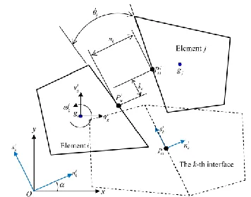
The discontinuous kinematically admissible velocity between two adjacent rigid elements in a typical upper bound analysis can now develop into two failure modes, namely, the simple sliding failure, which is controlled by the Mohr-Coulomb criterion, and the rotational failure, which is controlled by the new overturning criterion. A possible discontinuous kinematical admissible velocity ﬁeld at the interface is shown in Fig. 1 where Pm denotes the center of

the k-th interface between two typical rigid elements i and j. The discontinuous velocity can be conveniently measured by a strain rate vector as follows:

(1)

wherenk _,sk _and



k _{= relative tangential, normal, and angular displacement rates, at the center of the joint,} respectively. (2)

Figure 1. Kinematically admissible discontinuous velocity field of interface between two rigid elements

The discontinuous strain rate vectors at all interfaces of a discretized RFEM domain can be assembled into the following vector:

(2) where nd = number of all interfaces.

In local coordinates si

k -o- nik , the velocity at the center Pim of the kth interface caused by the centroid velocity of

ith element can be written as:

(3)

Where in the vector below:

(4)

ui = centroid velocity of the ith element; ui_{g and}_vi_{g = translational velocities in the x-and y-directions of the global} coordinates x-o-y; ωi_{g = rotational velocity of the}_i_{th element.}_N

i/k = RFEM shape function of the ith element

corresponding to the kth interface; and Li/k = matrix of direction cosines of the local sik-o- nik axes for the kth interface

with respect to the global coordinate system x-o-y. Speciﬁcally, Ni/k & Li/k are formulated as follows:

[ ]T

k nk sk k

  

1

[

, .... ,

_d

]

T T T T

n







/ / / i

i k L N ui k i k





[ i i i]

g g g

i

(3)

581

(5)

(6)

Likewise, similar deﬁnitions can be made for element j, and the difference of velocity between element i and j can then be found as:

The global velocity vector can be written as follows:

(8)

Its relation with the velocity of each specific element is written as follows:

(9)

The following selection matrices CiandCj for elements i and j are introduced:

(10)

Eq. (7) can then be reformulated as:

(11) Where

(12)

As a result, the global discontinuous velocity vector can be formulated as:

(13)

where

(14)

BT_{= strain rate matrix. The above formula represents the compatible condition between two adjacent rigid elements.}

This compatibility equation can be used to construct a numerical formulation for the consequent upper bound limit analysis.

Equilibrium Equations for Rigid Element

To apply the lower bound limit theorem, one needs to derive the equilibrium equation of rigid elements as well. Assume that the generalized stresses at the interface k of a rigid element involve the shear force Vk, the normal force

/g k/m

/ / /

1 0 y

0 1

0 0 1

i

i k k m i g

y

N x y

               /

cos( , ) cos( , ) 0 cos( , ) cos( , ) 0

0 0 1

i k

n x n y

L s x s y

          

1 1 ₍₃ ₁₎

T T T T

m _m

U u u u



 

 



( ) ( )

i j i j u  C U

3 ( ) 2 3 ( ) 1 3 ( )

( )

(3 3 )

0 0 1 0 0 0 0

0 0 0 1 0 0 0

0 0 0 0 1 0 0

i j i j i j

i j m C                    

k B Uk









/ / j / i

k i k j k i k

B  L N C  N C

B U





1 2

( 3m 3n )

d

T T T

T

n

B B B B



 

 

 



/

(

/ j / i

)

k

L

i k

N

j k

u

N u

i k

(4)

582

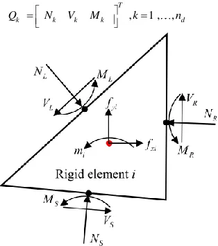
Nk, and the moment Mk , all applied at the center of the interface as shown in Fig. 2. They can be denoted in a vector

form as: (12)

(15)

Figure 2. Forces acting on one rigid finite element

The global stress vector can be written collectively as follows (formula 16):

(16)

According to the principle of virtual work, in a equilibrium system the external force along with the virtual displacement equals to internal energy waste. In RFEM, the energy for changing the form of system is stored between interfaces of the elements. There would be no stress occurred in rigid element and consequently there would be no energy waste inside the element. Therefore, the equation of principle of virtual work would be:

(17)

Substitution of Eq. (13) into Eq. (17) leads to:

(18)

Considering U 0 in general cases gives the following global equilibrium equation:

(19)

Where:

(20)

(21)

(21) Represents global external force vector to the i-th component. This equilibrium is the same as the one proposed by Ferris and Tin-Loi (2001). (3)

, 1 , ,

T

k k k k d

Q _N V M _ k n

 

 

1 2 d

T T T

T

n Q _Q Q Q _

 



0

T _Q _UT _F







   

0

T T T

U B Q U F

 

  

0 T

B Q F

  

1 2 , ,

T T T

T

m

F _ f f f _

 



T

m x i y i i

f _ f f m _

 

(5)

583

Yield Criteria and Flow Rules for Sliding and Rotation Mechanisms

The kinematical admissible discontinuous velocity derived in the Equilibrium Equations for Rigid Element section can be separated into two failure modes, namely, relative sliding and rotation of an element with respect to its adjacent element.

Accordingly, two different yield conditions are employed to govern the failures at the interface: a Mohr-Coulomb criterion for the sliding failure and an overturning failure criterion for the rotation failure.

Sliding Mechanism between Two Rigid Elements

Fig. (1), illustrates a translational sliding of element j over element i. Mobilization of this translational mechanism may be described by the Mohr-Coulomb criterion, i.e.

(21)

Note that compression is taken to be positive here. Based on the generalized stress deﬁned in Eq. (11), the above Mohr-Coulomb failure criterion may be recast to the following form:

(22)

where Δx = total length of interface. Note that the use of the absolute value of Vk indicates that the shear direction is

unrestricted.

Rotational Failure Mechanism between Two Rigid Elements

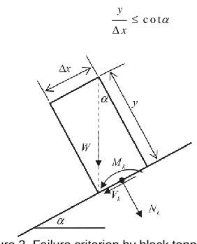
Element rotation has been ignored by previous RFEM-based limit analyses by other researchers and the main purpose was to maintain the condition of no gap or overlap between neighboring elements. Although it appears to be reasonable for the translation-dominant type of slope failure, the assumption proves to be inadequate to describe cases (such as upwelling underground water or increase in the height of soil slopes) where the rotation may be a contributing factor. The criterion is generalized based on the toppling failure criterion originally proposed by Goodman and Bray (1981). Consider a block on an inclined surface subjected to self-weight only (Fig. 3). Fig. 3 shows a state in which a rotation or toppling of the block is pending. The critical condition can be expressed as:

(23)

Figure 3. Failure criterion by block toppling

By multiplying both sides of the inequality in Eq. (24) with the weight W of the block, the following expression of the failure criterion is obtained:

(24)

t a n n

c

    

t a n 0

k k

V  N   c x

c o t

y

x  



0 , ,

2 2

k

k k k k

x W Sin y

(6)

584

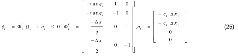
To facilitate the subsequent numerical implementation, the sliding failure criterion and the overturning failure criterion for the k-th interface can be collectively expressed in the following matrix form:

(25)

Where



k and

c

k = friction angle and cohesion at the k-th interface, respectively. The failure criteria at all interfaces can then be assembled in the following matrix formulation:

(26)

Where nd = number of interfaces in the discretized domain.

Associated Flow Rule

In conjunction with the previously given failure criteria, additional constraints on the kinematically admissible velocity field are needed by considering the associated flow rule. For interface sliding, the associated flow rule

assumes that the tangential velocity change,



, is accompanied by the separation velocity,

 

tan

(Fig. 4). As for the interface overturning, the associated ﬂow rule requires that the normal velocity change



corresponds to an

opening angle change of

2 /





x

(Fig. 4).

Figure 4. Sliding & Rotational Interface Failure modes between two rigid elements

In relation to the velocity vector in Eq. (1), these kinematic slip and rotation conditions can be expressed as Eg. (27):

t a n 1 0

0 1

0 , ,

0 2 0 0 1 2 k

k _k _k

T T k k

k k k k k k

c x

x _c _x

Q a a

x       _ _                                       _ _       d d d 1 2

( 1 4n )

1

2

( 4n 3n )

1 2

0

, . , . , . ,

0 0

0 0 0

0 0

0 0 0

,. ,. ,. ,

d

T

T T T

T n T T T T n

T T T

T

n Q a

a a a a

(7)

585

(27)

Assembling all the associated ﬂow equations for the interface gives:

(28)

In Eq. (28),



k _{vector is written as:}

(29)

Where



k _{= vector of nonnegative plastic multipliers. By substituting Eq. (28) into}



BU _{, the compatibility} condition can be reformulated as follows:

(30)

With previously given compatibility equation and equilibrium equation, the upper and lower bound limit analysis can be treated as a uniﬁed mathematical programming problem, which will be conducted in the Linear Programming for RFEM-Based Limit Analysis section. (2)

Linear Programming for RFEM-Based Limit Analysis

As shown previously, the kinematically admissible velocity field has been separated into sliding and rotational modes, and the relative rotation between two rigid elements is governed by the toppling failure criterion in Eq. (24). Following the assumption of the associated flow rule, the relative rotation is further introduced into the governing equations of the kinematically and statically admissible fields in the limit analysis. In addition, the compatibility, equilibrium, and failure equations formulated previously are all in linear form. Taking this feature, the authors can then formulate the upper and lower bound theorems into a dual of two linear programming problems.(5)

Primal Problem of Linear Programming for Kinematic Approach

The upper bound approach of limit theory states that any limit load multiplier λ for a kinematically admissible velocity restricted by the compatibility equation and associated ﬂow rule, i.e., Eq. (30), cannot be smaller than the plastic collapse multiplier λc, i.e., λ≤λc. An upper bound limit analysis aims to ﬁnd the minimum of the load multiplier

λmin to approximate λc. Using the associated ﬂow rule in Eq. (28) in the virtual principle in Eq. (17) gives the following

equation for the load multiplier:

(31)

Further substitution of the failure criteria in Eq. (27) into the previously revised virtual principle, leads to Eq. (34):

By

considering the complementary condition  T 0, the load multiplier can be formulated as follows:

(33)

As a result, the upper bound approach can be formulated as the following linear programming problem Eq. (34):

Notethat boundary conditions in the upper bound approach constitute mainly prescribed velocities, for example, 0

U _{. Although they do not contribute to the real velocity ﬁeld, the generalized primal variables in Eq. (34) will not}

include the quantities on the prescribed boundaries.

/

i k k Qi

      

k k k

    

1 , 2 , 3 , 4

T

k _k _k _k _k

     

 



B U  

0 T T_Q _{U F}T

   

, 1

T T

a W hen U F

 

(32)

(34)





0

T _a _{U F}T

   

 

,

1

min .

0

T T_a _{s t} U F

B U

 

 

   

 

(8)

586

Dual Problem for Static Approach

In the lower bound approach of limit theory, any load multiplier λ corresponding to a statically admissible stress ﬁeld constrained by the equilibrium equation and the failure criteria cannot be greater than the plastic collapse multiplier λc, i.e., λ≥λc. The linear programming problem of a lower bound approach is to ﬁnd the maximum of the load multiplier λmax. Alternatively, according to the dual theory of linear programming, the lower bound approach can be also formulated as the following dual of the primal

problem of the corresponding upper bound approach:

(35)

According to the duality theory of linear programming, the upper (primal) and the lower (dual) bound solutions can be found by solving the following optimal (Karush- Kuhn-Tucker (KKT)) conditions utilized in MOSEK (7) package:

(36)

The matrix contains , Q ,U ,



parameters which represent limit load multiplier, stress between elements, velocity of element and plastic multipliers respectively. To solve the matrix above, the boundary conditions and bound solutions must be satisfied by defining appropriate upper and lower limits for the unknowns in the matrix prior to solving the problem.

Satifying the boundary conditions

In solving the problem, we satisfy the boundary conditions by assuming the upper and lower boundaries of velocity parameters of stability elements as zero. Therefore, the programming and enhancement techniques are being implemented and optimum limit load multiplier  and other velocity parameters are calculated.

Evaluating the stability of soil slope

In previous sections, the formulation applied during the various phases of the research is comprehensively described. In this section, the problem and the edited algorithm is being evaluated using the programming algorithm used by Liu & Zhao, (2013) (2).

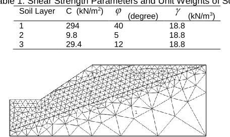
The problem is a soil slope with three different soil layers. The shear strength parameters and unit weight of each layer are also summarized in Table 1. The domain is discretized by an unstructured triangle mesh as shown in Fig. 5. (6)

Table 1. Shear Strength Parameters and Unit Weights of Soils

Soil Layer C (kN/m2₎



(degree)



(kN/m3₎

1 294 40 18.8 2 9.8 5 18.8 3 29.4 12 18.8

Figure 5. Typical rigid ﬁnite-element mesh for the inhomogeneous slope using COSMOL software

 

0

max .

0 T

T

B Q F

s t

Q a

 



  

 

   

0 0 0 0 1

0

0 0 0 0

0

0 0 0 0

0

0 0 0

T

F

B Q

w h e r e

F B U

a



   

 

       

 _

       



         _

           

          

        _ 

 _     _   _ 

(9)

587

The method of reducing strength has been employed to ﬁnd the factor of safety for this problem, by following the common deﬁnition of the factor of safety:

(37)

Where cand



= effective cohesion and internal frictional angle, respectively; and cm _and



m _{= reduced} (mobilized) cohesion and frictional angle, respectively.

The factor of safety Fs is computed in conjunction with optimization of the limit load multiplier λ according to Eq.

(36). Speciﬁcally, an initial value Fs (usually a small one) is chosen ﬁrst to calculate the reduced cohesion and

frictional angle cm _and



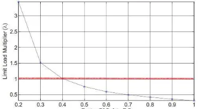
m _{according to Eq. (37). These two strength parameters are substituted into Eq. (26) to obtain} an optimal limit load multiplier λ using the proposed method and MOSEK software. The process is repeated by gradually increasing the value of the factor of safety from its initial value. Consequently, a series of limit load multipliers in conjunction with the corresponding factor of safety can be obtained, which can be plotted in a ﬁgure like Fig. 6. The ultimate factor of safety for the problem corresponds to the value at the intersection of the curve with m the horizontal line λ =1.

Figure 9. Determination of the factor of safety by optimizing limit loading multiplier

As is summarized in Table 2, in particular, the factor of safety in consideration for both sliding and rotation failure modes is found between the upper bound and lower bound obtained in this research and is compared with the results obtained by Spencer’s method along with the results obtained by (Liu & Zhao, 2013) (2).

Table 2. Comparison of Factor of Safety by Various Methods

s F

Methods Authors

0.41 Spencer’s method

Present method

0.38 Janbu method

Present method

0.47 Limit Analysis (LimitState:GEO) Present method

0.405 RFEM-based limit analysis

Present method

0.421 RFEM-based limit analysis

Liu & Zhao, 2013

As the table shows, the obtained factor of safety from RFEM-based limit analysis methods is in the range of other methods. The resulted algorithm (with 4% variation) has an appropriate conformity with Liu & Zhao (2013) results.

Fig. (7) shows Kinematically admissible velocity ﬁelds. the arrows show the direction of velocity vectors in the model.

Figure 7. Kinematically admissible velocity ﬁelds obtained Limit Analysis t a n

t a n s

m m

c F

c

 

 

 

(10)

588

Fig. (8) shows the sliding line obtained from SLOPE/Win comparison with LimitState:GEO. The dashed line is the result of SLOPE/W software and the solid line for LimitState:GEO.

Figure 8. Comparison of Sliding line results of SLOPE/W & LimitState:GEO for the inhomogeneous slope problem

The failure line obtained by LimitState:GEO software (solid line) shows that the soil slope at the upper part of Soil #2 (middle layer) has more penetration and consequently, is close to the result of SLOPE/W software. But in other parts, these 2 results are close to each other. Meanwhile, the failure lines of Janbu, Spencer and other methods are all close to the dashed line in Fig. (8).

Implementing sensitivity analysis on parameters

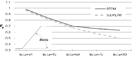
For all the Analysis performed in this section, the variation of Factor of safety against the changes of geometrical parameters such as angle of slope and height of the block for the Soil #3 (Table.1) are being assessed. Also, the variation of Factor of safety against mechanical parameters changes of the soil such as internal friction angle and soil cohesion (when the internal friction angle is constant) is being evaluated. For comparison, Janbu method has been used in order to analyze the results by SLOPE/W software.

Figure 9. Changes of Factor of Safety versus slope angle changes

The results show that the Factor of Safety difference (variance) in 2 above method is 2% from Angle 34° to 60°. The variance increases as the slope angle goes beyond 60°.

Fig. (10), shows the changes in soil cohesion and its effect on Factor of safety. The results show that the difference of Fs amounts in the two compared methods widens as the soil cohesion increases.

Figure 10. Changes of Factor of Safety versus soil cohesion (with constant internal friction angle)

Conclusion and results of the introduced method

(11)

589

in large scale and numerous elements. One of the issues in solving this problem was the non-convergence of Factor of safety results. Better defining the Matrix of direction cosines and better meshing was very effective in solving the problem correctly. Future study will focus on the enhancing Rotational failure criterion and its improvement for being used in rock slopes.

REFERENCES

Cheng YM and Lau CK. 2008. “Slope Stability Analysis and Stabilization”. USA, Routledge.

Fentago L and Jidong Z. 2013. “Limit Analysis of Slope Stability By Rigid Finite Element Method And Linear Programming Considering Rotational Failure”. Int. J. Geomechanics, ASCE.

Ferris MC and Tin-Loi F. 2001. “Limit Analysis of Frictional Block Assemblies as a Mathematical Program with Complementarity Constraints”, Int. J. Mechanical Sciences.

Goodman RE and Bray JW . 1981. “The theory of base friction models”. Int. J. Rock Mech. Min. Sci. & Geomec.

Kim J, Salgado R and Lee J. 2002. “Stability Analysis of Complex Soil Slopes using Limit Analysis “. Journal Of Geotechnical And

Geoenvironmental Engineering, ASCE.