Solving Queueing Network Models in Cloud Provisioning
Contexts
Marta Beltran and Francisco Carriedo
Department of Computing, ETSII
Universidad Rey Juan Carlos
28933, Madrid (Spain)
[email protected] and [email protected]
ABSTRACT
In recent years the research community and most of cloud users are trying to propose flexible and general mechanisms to determine how much virtual resources need to be allo-cated to each tier of the applications executed on cloud in-frastructures. The objective of this virtual provisioning is twofold: minimizing resources consumption and meeting the service level agreement (SLA). Most of the current cloud provisioning and scaling solutions are based on analytical models of applications, trying to automate the provision-ing decisions makprovision-ing ”what-if” response time predictions. Queueing network (QN) models have demonstrated to be a good choice in this kind of contexts. In this work we compare, performing an exhaustive set of experiments on a real cloud architecture with a new provisioning mechanism, exact solutions with approximate solutions estimated from bounding techniques in order to obtain conclusions about the most efficient way of solving these models when making cloud provisioning decisions.
Categories and Subject Descriptors
Mathematics of Computing [Probability and Statistics]: Queueing theory
General Terms
Experimentation, Performance
Keywords
Balanced Job Bounds, Cloud Provisioning, Mean Value Anal-ysis, Queueing networks
1.
INTRODUCTION
Cloud architectures provide the illusion of infinite com-puting resources and their elasticity frees developers, de-signers and in general, end users, from the confinement of traditional in-house systems. However it also makes these users responsible for requesting their providers the necessary amount of resources (depending on the demand at any given time) to obtain the required performance at minimum cost. This is why different automatic solutions are being proposed to help end users in making fast and efficient provisioning decisions.
These automatic solutions use to rely on application mod-els that estimate the average response time or the average throughput of the application in order to make provisioning decisions, minimizing costs and correcting in the run time the possible deviations from the SLA. In this paper we dis-cuss and compare the two main different approaches used to estimate the average response time of cloud applications in order to make provisioning decisions (independently on who is making these decisions: providers, brokers or end users) when these applications behaviour is modeled with a queue-ing network: exact and approximate solution techniques.
The main contributions of this work are summarized as follows (a) We have analyzed the previous work in pre-dicting the average response time of applications executed on cloud environments to draw conclusions about the most widespread QN models and solving techniques (b) Taking as a basis all these conclusions, two techniques have been considered for comparison, one exact technique (Mean Value Analysis or MVA) and one approximate technique (Balanced Job Bounds or BJB) (c) We have designed and implemented a new flexible and general provisioning solution to automat-ically scale the virtual resources needed to execute a n-tier application executing on a cloud environment (d) We have compared the two considered techniques with an exhaus-tive set of experiments performed with a 1-tier scientific and a multi-tier interactive benchmark executed on a pri-vate cloud.
The remainder of this paper is organized as follows. Sec-tion 2 discusses the most important related works. SecSec-tion 3 gives a detailed description of the considered problem and assumptions. Section 4 describes the proposed provision-ing mechanism and summarizes the most important results obtained in all the performed experiments. And finally, Sec-tion 5 presents the most important conclusions of this work and some suggestions for future research.
3HUPLVVLRQWRPDNHGLJLWDORUKDUGFRSLHVRIDOORUSDUWRIWKLVZRUNIRU SHUVRQDORUFODVVURRPXVHLVJUDQWHGZLWKRXWIHHSURYLGHGWKDWFRSLHV DUHQRWPDGHRUGLVWULEXWHGIRUSURILWRUFRPPHUFLDODGYDQWDJHDQGWKDW FRSLHVEHDUWKLVQRWLFHDQGWKHIXOOFLWDWLRQRQWKHILUVWSDJH7RFRS\ RWKHUZLVHWRUHSXEOLVKWRSRVWRQVHUYHUVRUWRUHGLVWULEXWHWROLVWV UHTXLUHVSULRUVSHFLILFSHUPLVVLRQDQGRUDIHH
9$/8(722/6'HFHPEHU%UDWLVODYD6ORYDNLD &RS\ULJKWk,&67
'2,LFVWYDOXHWRROV
2.
RELATED WORK
2.1
On cloud provisioning
Most of the current provisioning and scaling solutions are based on analytical models of the applications executed on the cloud infrastructure, automating the decisions and bas-ing them on response time predictions, releasbas-ing the agents responsible for provisioning (provider, broker or end user, it depends on the context) of making these decisions based on their own predictions or on complex static rules. Specif-ically, many authors have decided to model general n-tier cloud applications as queueing networks in order to achieve an appropriate balance between accuracy and cost; separa-ble queueing networks are the most widely used.
These authors have enumerated and discussed the rela-tionship between the inputs (basically user description, server description and service demand) and the outputs (basically average response time, system throughput and average queue lengths) of separable queueing network models. Many works (for example [2], [3], [11] or [13]) rely on exact solution tech-niques, such as the Mean Value Analysis, or on accurate solution techniques such as iterative bounds, to predict the average response time or the average throughput of different application configurations. And with this exact, or at least accurate solutions, provisioning decisions are made for the different tiers.
But one of the main advantages of the QN models is that it has been demonstrated that it is possible to determine up-per and lower bounds on the aforementioned up-performance measures with a very low cost. In fact, they are so simple to calculate that they can be estimated even by hand. The exact or iterative bounding techniques provide accuracy but require considerably more resources, specially when the re-sults are needed in real time and the system architectures are large and complex. Such benefits have made last works ([5], [6], [9] or [12], for example) to favour computational effi-ciency over solution accuracy using another types of bound-ing and heuristic techniques.
To the best of our knowledge this evolution from exact to approximate solutions has not been justified with an ex-perimental evaluation. The effects that the loss of accuracy in the model solution may have on provisioning decisions quality have not been quantified yet. In this work we want to find to what extent the QN models solution can be ap-proximated to favour the desired computational efficiency without leading to over-provisioning or under-provisioning scenarios.
2.2
On solving QN models
Mean Value Analysis (MVA) [7] is an efficient algorithm designed to analyze product form queueing networks and to obtain mean values for queue lengths and response times, as well as throughputs. However, the computational com-plexity of this exact solution technique and of the accurate iterative bounding techniques derived from it made neces-sary more simple and fast bounding techniques.
There are three kinds of simple bounds for the typical per-formance figures: asymptotic, balanced jobs and geometric bounds. These bounding techniques provide non-iterative lower and upper bounds for the model outputs with a com-putational cost independent of the population size L (which is the most important source of complexity in the exact
solu-tion computasolu-tion). That is the reason why these techniques are often called single-step techniques.
The asymptotic bounds consider the extreme scenarios of light and heavy loads (the most optimistic and pessimistic situations respectively) while the balanced job or balanced system bounds (BJB) assume balanced systems meaning this balance that the service demand at every server in one specific tier is the same [14]. With a few additional cost, balanced job bounds are more accurate than the asymp-totic. Finally geometric bounds [4], derived by describing the queue-lengths with a geometric sequence of terms re-lated to the resource utilization, obtain similar results than balanced job bounds in terms of accuracy. This technique implies similar computation costs than the Balanced Job Bounds but it does not demand the system balance require-ment, which can be an important advantage in certain ap-plication architectures.
Analyzing the previous work in the area of cloud provi-sioning, two different kinds of techniques are being widely used to solve the queueing models used to predict the av-erage response time with different configurations of the ap-plication tiers: the Mean Value Analysis to obtain exact solutions and balanced job bounds to obtain approximate solutions (because many of the mentioned provisioning so-lutions such as [2], [6] or [9] assume that all the virtual ma-chines composing an application tier are homogeneous and perfectly or near perfectly balanced). Therefore, this work tries to compare the results obtained with these two kinds of techniques, MVA and BJB.
3.
CONSIDERED PROBLEM
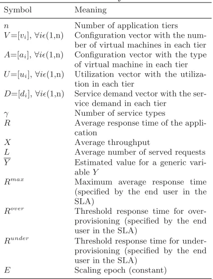
The notation used in the rest of this paper is summarized in table 1. This work considers the following assumptions regarding cloud providers and end users:
• End users submit requests to an application cloud provider owning a n-tier application which can be batch or in-teractive.
• The application cloud provider owns the physical in-frastructure or depends on a IaaS provider, it is indif-ferent for our analysis.
• End users and the application cloud provider agree on a probabilistic application-SLA based on the max-imum average response time allowed for the applica-tion.
• The application cloud provider can reject an end user’s request if the response time for this request is predicted to fail in meeting the SLA.
• End users want to meet their SLA minimizing the number of provisioned virtual machines. The opti-mization problem to be solved with the application provisioning can be expressed as:
Minimize
n
i=1
vi (1)
with the SLA constraint R < Rmax (2)
Table 1: Summary of notations
Symbol Meaning
n Number of application tiers V=[vi],∀i(1,n) Configuration vector with the
num-ber of virtual machines in each tier A=[ai],∀i(1,n) Configuration vector with the type
of virtual machine in each tier U=[ui],∀i(1,n) Utilization vector with the
utiliza-tion in each tier
D=[di],∀i(1,n) Service demand vector with the
ser-vice demand in each tier γ Number of service types
R Average response time of the appli-cation
X Average throughput
L Average number of served requests Y Estimated value for a generic
vari-ableY
Rmax Maximum average response time (specified by the end user in the SLA)
Rover Threshold response time for
over-provisioning (specified by the end user in the SLA)
Runder Threshold response time for
under-provisioning (specified by the end user in the SLA)
E Scaling epoch (constant)
Note that we have considered a SLA based on a con-straint to the average response time of the application. The user will obtain an acceptable service in her per-ception if this average response time is always kept under the value specified byRmax.
The following models can help in understanding the rest of this work, we have found that these models are repre-sentative of the most common scenarios and therefore, the conclusions obtained in the further experimental analysis can be generalized.
Application and service model.
The application provider owns a n-tier application, each tier providing a specific functionality to its preceding tier in the form of a processing pipeline. If the application contains database tiers, we assume a shared-everything architecture which can be clustered and replicated on demand. The work-load of the multi-tier application is typically session-based, where an end user session consists of a succession of service requests. At a time, different concurrent service requests from different end users interact with the multi-tier appli-cation. In this work we focus on batch and interactive ap-plications, therefore on closed models in which end users re-circulate.
We consider an application withγservice types, this means that an end user request not always implies executing the same workload on each tier, the path from tier 1 to tier n can be crossed in several ways and there is nota priori
knowledge about the proportion in which each of these ser-vice types are requested. Serser-vice requests can join and leave
the system at any time and each request at tierican trigger zero or multiple requests to tieri+ 1.
Regarding the infrastructure, we assume a fairly normal scenario: the infrastructure provider offers different types of virtual machines in the form of predefined virtual appliances or machine images. There areviidentical virtual machines
in the tier i, but one tier may be composed of virtual ma-chines of a different type than other.
According to these models, each virtual machine in each tier can be modeled as a -/G/1/PS queue. This model is rep-resentative of the considered scenario as it has been in pre-vious works (for example [6], [9], [10] or [13]). Since we want to model arbitrary multi-tier applications with an arbitrary number of tiers, we cannot make assumptions about service requests arrival rate. Note that the service times of the pro-visioned virtual machines follow a general distribution and the only requirement on this service time distribution is that it must have rational Laplace transform. This includes all distributions which can be expressed as a network of expo-nential stages, therefore it is not a strict limitation. And finally, service requests are forwarded to the running queue of virtual machines in the different application tiers, which process these requests following processor sharing strategies (PS).
Provisioning model.
We assume that virtual machines can be requested and terminated by end users at any time, and billing is based on the amount of time that each virtual machine has been used. For simplicity, the provisioning mechanism is assumed to be on the provider’s resources, allowing an end user to contract the automatic provisioning service to the provider. This mechanism allows one to apply horizontal scaling for each application tier. This implies adding or releasing virtual machines in one tier without modifying the type of machine provisioned for this tier. This kind of scaling changes only the number of machines in tieri, i.e. vi.
4.
EXPERIMENTAL ANALYSIS
In order to compare the two selected techniques, MVA (exact solution) and BJB (approximate solution), on cloud provisioning contexts, a private cloud has been deployed and a new general provisioning mechanism based on horizontal scaling has been designed and implemented. Specifically, we are interested in assessing the behaviour of the two QN models solution techniques with n-tier applications, with one type of service or multi-class (γtypes of services), and con-sisting of batch or interactive workloads.
4.1
Provisioning solution
The solution designed to perform the experimental evalu-ation is composed of three different modules: a Controller, an Informer and a Scaler, this last module responsible for the response time prediction solving the QN model with MVA or BJB. A load Balancer is needed in each tier too, but it is not part of the provisioning solution.
The Controller module has been designed to make admis-sion control deciadmis-sions following the ideas presented in [8]. The admission control considers the Acceptable Risk Level (ARL) to make decisions, defined as the probability of hav-ing insufficient capacity to satisfy a client’s SLA.
Once a service request is admitted by the Controller mod-ule it is sent to the load balancer of tier 1. Although this
module is not strictly part of the provisioning solution, each tier needs a Balancer to optimize the usage of the virtual re-sources provisioned for a user distributing the workload in a balanced and even way after accepting new service requests or after implementing the configuration changes suggested by the Scaler module. The Balancer module must be de-signed and/or configured in each tier to obtain the same utilization degree (or as close as possible) in all the virtual machines composing the tier. This task is not very com-plicated due to the homogeneity of these virtual machines in each tier, although the possible heterogeneity in service requests has to be considered.
The Informer module gathers in runtime, using the provider’s network and communication resources and mechanisms, all the data and information needed to automate the provision-ing decisions, mainly related to physical resources utiliza-tion, virtual machines utilizautiliza-tion, application configuration and behaviour and overheads (specifically, load balancing overheads). To implement this module usual system inter-faces to access to the operating system performance data (such as the /proc filesystem) on each system node and virtual machine can be used. In addition some users and providers may implement their own kernel modifications to increase the measurement speed and to decrease the level of intrusiveness if needed.
The Scaler module periodically evaluates (with the scal-ing epoch E) the application behaviour to decide whether a horizontal scaling has to be performed. As it has been mentioned before, the horizontal scaling (or scaling out) in-creases or dein-creases the capacity of a tier by adding or re-leasing individual virtual machines depending on the appli-cation response time and on the thresholds defined by the end user in the SLA.
The Scaler is responsible for computing at each epoch the number of virtual machines that need to be provisioned at each tier so that the application response time is main-tained below the threshold given byRmax. But it is also
re-sponsible for avoiding unnecessary costs by preventing over-provisioning scenarios and by minimizing the changes in con-figurations. As it can be seen in algorithm 1, the Scaler first checks if the response time of the application is below the threshold given by the user to identify over-provisioning scenarios and therefore, to release virtual machines with the ReleaseVM function. After this, the Scaler checks the op-posite situation: if the response time is above the threshold given by the end user to identify under-provisioning situa-tions (in these scenarios it is very likely that the response time constraint is not fulfilled), new virtual machines are needed in the bottleneck tiers. In these cases the CreateVM function is invoked.
The ReleaseVM function identifies all the tiers which can be candidates to a scaling down process. After that, the new configuration is iteratively computed removing one virtual machine at a time from the most under-utilized tier in each iteration. Then the RPrediction function (explained later in this paper) is used to estimate the application response time after each change and to decide whether or not the scaling down of the selected tier can be performed.
The CreateVM function is an iterative function too. In this case, at each iteration the bottleneck tier with the high-est utilization value must be identified. A single new virtual machine is added to this tier, and the average response time of the application is estimated with the RPrediction
func-Algorithm 1Pseudocode for the Scaler module
Require: E(constant)
Require: Rover, Runder and Rmax (specified by the end
user)
Require: R,X,UandV (from the Informer module)
Ensure: V
1: while(1)do
2: Vold=V;
3: if R < Roverthen
4: V=ReleaseVM(R,X,U,Vold);
5: end if
6: if R > Runderthen
7: V=CreateVM(R,X,U,Vold); 8: end if
9: if V =Voldthen
10: Perform scaling; 11: end if
12: sleep(E); 13: end while
Algorithm 2 Pseudocode for the RPrediction function based on the BJB technique
Require: L,Dq∀q(1, γ) andV
Ensure: RandU
1: qbest= [q|min(ni=1dqi)]∀q(1, γ); 2: qworst= [q|max(ni=1dqi)]∀q(1, γ); 3: dbest
total=
n
i=1dqbesti ;
4: dworsttotal=ni=1dqworsti ; 5: vtotal=n
i=1vi;
6: mdbest
mean=dbesttotal/vtotal;
7: mdworstmean=dworsttotal/vtotal;
8: mdbest
max=max(dqbesti /vi);
9: mdworst
max =max(dqworsti /vi);
10: R+=dworsttotal+(L−1)mdworstmax ; 11: R−=max(Lmdbest
max,dbesttotal+ (L−1)mdbestmean);
12: R= R++R−
2 ;
13: X+= min
1
mdbestmax,
L dbesttotal+(L−1)mdbestmean
; 14: X−= L
dworsttotal + (L−1)md worst max ;
15: X= X++X−
2
16: fori= 1→ndo
17: ui=Xdi;
18: end for
tion. These stages are iterated until the response time is below the under-provisioning threshold,Runder.
RPrediction function.
Two RPrediction functions have been developed in this work, the first one based on the MVA technique (exact solu-tion) and the second, based on the BJB technique (approx-imate solution).
The RPrediction function based on the Mean Value Anal-ysis technique has been implemented with a direct trans-lation of the algorithm provided in [7]. The response time prediction with this version of the RPrediction function has a computational complexity O(γnL).
The algorithm 2 shows the RPrediction function based on the Balanced Job Bounds technique, considering the multi-class case when there are different types of services. The
application response time and the throughput are estimated as the average value of the upper and lower bounds provided by the BSB algorithm described in [14]. In this case, the computational complexity of the response time prediction is O(γn), independent of the populationL.
Note that, since there are multiple service types, multi-ple sets of input parameters (one set per type) should be required. But most current measurement tools and APIs do not provide sufficient information to determine the input pa-rameters appropriate to each service class and, furthermore, we are assuming noa priori knowledge about the propor-tion of the different kinds of service requests. To overcome these limitations, the trivial solutions of balanced networks have been used [14], solving the balanced network using the best and the worst values considering all the service types possible in the system.
This RPrediction function is going to be used to obtain response time estimations for both batch and interactive ap-plications. For batch workloads, the bounds on average re-sponse time are straight lines and also the optimistic bounds on average response time for interactive workloads. How-ever, the pessimistic bounds on response time for interac-tive workloads are not linear inL, and thus they should be computed separately for each value ofLtaking into account the value ofZ, the think time quantifying the average time that users use terminals (ˆa ˘AIJthinkˆa ˘A˙I) between interac-tions. To avoid this overhead, only optimistic bounds will be considered in this work, leading perhaps to a certain degree of under-provisioning that will have to be correctly man-aged by the designed provisioning mechanism but choosing the simplest solution possible.
4.2
Experimental setup
All the experiments have been performed with commod-ity hardware. Up to 16 machines have been used to build a private cloud infrastructure with Xen/Linux. The 16 servers included in the cloud infrastructure are connected by a Gi-gabit Ethernet network and a different machine is used to emulate the users and to generate all service requests. A spe-cific server has run the provisioning solution (Core i7 3820, 3.60 GHz with 32 GB of RAM) while the load balancer in each tier has been implemented with a distributed approach based on agents running on each virtual machine. Because resource provisioning (allocation of VMs to physical servers) is not the focus of this work, it has been implemented with a straightforward strategy, with all the servers running all the time and creating new VMs always on the physical host with fewer running machines.
For simplicity one VM type has been offered to the end users with 2 virtual CPUs, 2 GB of memory and 80 GB of storage capacity. Three different load scenarios have been considered and evaluated during 30 minutes, the first one with low levels of workload, the second one with moderate levels of workload and the third, with large levels (these lev-els and the correspondent arrival rates have been set attend-ing to the number of requests per minute of real applications and benchmarks not detailed here for space restrictions).
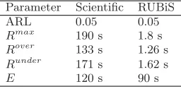
Table 2 summarizes the values of all the parameters used in the presented experiments. Some of these values, as well as information about the resources consumption that the Controller module needs to be configured, have been ob-tained by performing some initial experiments and tests. For example,Roverhas been fixed as a 70% ofRmaxandRunder
Table 2: Parameters used in the experiments
Parameter Scientific RUBiS ARL 0.05 0.05 Rmax 190 s 1.8 s Rover 133 s 1.26 s
Runder 171 s 1.62 s
E 120 s 90 s
as a 90% because after a proper tuning of the provisioning solution, these values have demonstrated to obtain good re-sults (trade-off between performance and overhead) with the considered benchmarks. In the same way, the values for the rest of constants have been determined (ARL andE).
Two applications have been selected for our experiments. The first,scientificfrom now, is a scientific workload consist-ing of submission of requests for execution of computation-ally intensive tasks (image rendering) on the service provider infrastructure. Therefore, it is a batch application (its in-tensity can be specified with the average number of active jobs or users) with one tier and only one kind of service.
The second is RUBiS [1], a three-tier web benchmark that represents an auction site similar to eBay comprising of a web server tier, an application server tier and a database tier (n= 3). This benchmark allows to simulate the activity of the auction site implementing three types of user sessions (selling, browsing and bidding) with 26 interactions that can be accessed from the client’s web browser. Therefore, it is an interactive or terminal application (its intensity can be specified with two parameters, the number of active termi-nals or users and the average length of time that customers use terminals or think between interactions).
4.3
Results and discussion
Tables 3, 4, 5 and 6 summarize the results obtained with our experiments. Each experiment has been conducted five times to report the average for each output metric. Out-put metrics collected for each experiment have been: quests arrival rate, average response time of accepted re-quests, standard deviation of response times among all ac-cepted requests, provisioning overhead, VM minutes, num-ber of performed application scalings, percentage of rejected requests (remember that the Controller module can reject service requests if the probability of having insufficient ca-pacity to satisfy the user’s SLA is above certain threshold) and number of requests served with under-provisioning re-sulting in a response time aboveRmax.
The average overhead introduced by the provisioning so-lution performing the automatic reconfigurations has been quantified measuring the total time consumed by the Scaler module execution and by the tiers reconfiguration (down-scaling or up-(down-scaling, depending on the situation). It has to be noted that the time needed to execute one response pre-diction with the RPrepre-diction function is only a fraction of a second, being quite small the observed difference between the MVA and the BJB versions. The total overhead have been measured instead, because it is the repetitive execution of this prediction inside the Scaler module (when the Relea-seVM and CreateVM functions are invoked) that makes the difference between the two evaluated techniques.
VM minutes is the sum of the wall clock time of each in-stantiated application, from its creation to its destruction.
Table 3: Time and configuration results obtained with the scientific benchmark
Scenario Min-Max requests/min Average R R std. dev. Overhead Low workload MVA 5-50 160 s 4 s 15 s Low workload BJB 5-50 159 s 3 s 12 s Moderate workload MVA 60-150 162 s 4 s 26 s Moderate workload BJB 60-150 163 s 4 s 17 s Large workload MVA 200-500 164 s 5 s 34 s Large workload BJB 200-500 166 s 6 s 22 s
Table 4: Cost and performance results obtained with the scientific benchmark
Scenario VM minutes Scalings % rejections Under-provisioned req. Low workload MVA 127 1 0.01 1
Low workload BJB 130 1 0.01 1 Moderate workload MVA 201 3 0.04 1 Moderate workload BJB 206 2 0.05 2 Large workload MVA 553 4 0.06 3 Large workload BJB 566 4 0.09 3
Table 5: Time and configuration results obtained with the RUBiS benchmark
Scenario Min-Max requests/min Average R R std. dev. Overhead Low workload MVA 50-120 1.52 s 0.08 s 43 s Low workload BJB 50-120 1.55 s 0.10 s 35 s Moderate workload MVA 100-300 1.53 s 0.10 s 54 s Moderate workload BJB 100-300 1.55 s 0.12 s 41 s Large workload MVA 500-1200 1.56 s 0.11 s 85 s Large workload BJB 500-1200 1.57 s 0.15 s 58 s
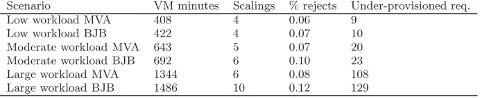
Table 6: Cost and performance results obtained with the RUBiS benchmark
Scenario VM minutes Scalings % rejects Under-provisioned req. Low workload MVA 408 4 0.06 9
Low workload BJB 422 4 0.07 10 Moderate workload MVA 643 5 0.07 20 Moderate workload BJB 692 6 0.10 23 Large workload MVA 1344 6 0.08 108 Large workload BJB 1486 10 0.12 129
This metric has been used before [3] as a metric for VM utilization and cost, because it allows to provide a measure-ment for cost that is independent from billing models applied by different cloud providers and makes the results easier to interpret and to compare.
First of all, the behaviour of the provisioning mechanism designed to perform the experiments can be verified. The proposed automatic solution is able to dynamically increase the number of virtual machines allocated to each applica-tion tier during workload spikes and to reduce it in off-peak moments in the three evaluated scenarios with both, MVA and BJB based response time prediction and for the two very different selected benchmarks. The number of virtual machines active in each tier has suffered important varia-tions maintaining an optimum average response time with an acceptable standard deviation, insignificant rejection and under-provisioning rates and always meting the SLA. These points validate the use of the -/G/1/PS queue model in the context of the considered problem and demonstrate its scal-ability. By scalability we mean the capacity of the solution to reasonably maintain its performance (average response
time observed by the user, overhead, etc.) when the number of received requests per minute increases.
The results obtained with the scientific application are very similar with the two versions of the RPrediction func-tion. The BJB technique obtains only marginally worse re-sults in terms of cost and performance than the MVA tech-nique because it is a one-tier batch application with only one kind of service, and therefore the approximate solu-tion obtained from the estimated bounds for R are accu-rate enough to make good provisioning decisions. Besides, the MVA technique introduces more overhead than the BJB technique, specially in the large workload scenario (remem-ber that the computational complexity of this technique de-pends on theLvalue), and all this means that the RPredic-tion funcRPredic-tion based on the BJB technique would be always the best option to solve the QN application model.
In contrast, the results obtained with the RUBis bench-mark show important differences between the two evaluated techniques. Note that this scenario is much more challeng-ing than the first: a multi-tier interactive application with different types of services. In fact, the proposed provisioning solution has been able to keep almost the same average
sponse time in all the experiments, but always a little worse when using the BJB technique. Another interesting trend that our experiments show is that this difference is also ob-served when comparing VM minutes, the number of scal-ing, the percentage of rejections and the number of under-provisioned requests. Summarizing, in these experiments the decisions made with the MVA technique lead always to better provisioning scenarios in terms of cost and perfor-mance. For example, if such an important difference can be observed in the VM minutes during a 30 minutes execution, the difference in costs that in a real scenario would involve the use of the BJB technique instead of the MVA technique could be critical.
With the BJB technique our solution keeps the response time observed by the user always near toRunder, being then
most likely the up-scalings than the down-scalings. This is because the bound used to predict the multi-tier application response time is always the optimistic one, and this leads to large virtual machines utilization values (ui values above 80% have been measured in all the performed experiments) but suffering greater risk of observing under-provisioning sit-uations. This is the reason why in all the experiments the scalings (specifically, up-scalings) have happened more fre-quently. And as it was to be expected, as the workload of the experiment scenario increases, the number of the needed scalings increases too.
The inconvenient in the case of the MVA-based solution is that it introduces more overhead than the BJB technique, even performing less tier reconfigurations, due to the larger computational complexity of this exact technique and there-fore to the larger time consumed in executing the RPredic-tion funcRPredic-tion. Again this has been specially important in the large workload scenario (large values ofL). With the BJB version, on the other hand, the average overhead has been kept always under the minute although this overhead has slightly increased in the most loaded scenarios.
5.
CONCLUSIONS AND FUTURE WORK
Although the utilization of single-step bounding techniques to solve QN application models in provisioning environments for n-tier cloud applications has several benefits, there are still challenges that need to be faced. Our experiments with two different kinds of applications performed on a Xen/Linux-based private cloud demonstrate the suitability of the BJB technique to solve QN models of cloud applications in pro-visioning scenarios where these applications are batch and a nearly perfect system balance can be ensured. But in the case of more complex scenarios (specifically, multi-tier in-teractive applications with different types of services) the approximations made ˆa ˘A ´Nˆa ˘A ´Nwith this type of technique lead to provisioning decisions not accurate enough for many users and contexts. As the computational cost of the MVA technique can become excessive in these same scenarios, it will be necessary to evaluate other approximate/bounding solutions for such situations.
Currently we are working in considering the heterogeneous case (different types of virtual machines in the same tier), in extending our experiments to larger and more complex ar-chitectures (using the simulation framework CloudSim) and in evaluating the geometric bounds technique, likely more suitable for complex scenarios and when the system balance assumption cannot be made.
6.
ACKNOWLEDGMENTS
This research has been partially supported by the Gov-ernment of Spain (Grant Ref. TIN2011-28151).
7.
REFERENCES
[1] RUBiS: Rice University Bidding System. http://rubis.ow2.org/.
[2] J. Bi, Z. Zhu, R. Tian, and Q. Wang. Dynamic provisioning modeling for virtualized multi-tier applications in cloud data center. InProceedings of the IEEE 3rd International Conference on Cloud
Computing, pages 370–377, 2010.
[3] R. N. Calheiros, R. Ranjan, and R. Buyya. Virtual machine provisioning based on analytical performance and QoS in cloud computing environments. In
Proceedings of the 2011 International Conference on Parallel Processing, pages 295–304, 2011.
[4] G. Casale, R. Muntz, and G. Serazzi. Geometric bounds: A noniterative analysis technique for closed queueing networks.IEEE Transactions on Computers, 57(6):780–794, 2008.
[5] E. Casalicchio, D. A. Menasc´e, and A. Aldhalaan. Autonomic resource provisioning in cloud systems with availability goals. InProceedings of the 2013 ACM Cloud and Autonomic Computing Conference, pages 1:1–1:10, 2013.
[6] M. Marzolla, S. Ferretti, and G. D’Angelo. Dynamic resource provisioning for cloud-based gaming infrastructures.Computers in Entertainment, 10(3):4:1–4:20, 2012.
[7] M. Reiser and S. S. Lavenberg. Mean-value analysis of closed multichain queuing networks.Journal of the ACM, 27(2):313–322, 1980.
[8] B. Rochwerger, D. Breitgand, E. Levy, A. Galis, K. Nagin, I. M. Llorente, R. Montero, Y. Wolfsthal, E. Elmroth, J. C´aceres, M. Ben-Yehuda,
W. Emmerich, and F. Gal´an. The reservoir model and architecture for open federated cloud computing.IBM Journal of Research and Development, 53(4):535–545, 2009.
[9] U. Sharma, P. Shenoy, and D. F. Towsley. Provisioning multi-tier cloud applications using statistical bounds on sojourn time. InProceedings of the 9th International Conference on Autonomic Computing, pages 43–52, 2012.
[10] L. Siew Huei and S. Ya-Yunn. CloudGuide: Helping users estimate cloud deployment cost and performance for legacyweb applications. InProceedings of the IEEE 4th International Conference on Cloud Computing Technology and Science, pages 90–98, 2012.
[11] B. Urgaonkar, P. Shenoy, A. Chandra, P. Goyal, and T. Wood. Agile dynamic provisioning of multi-tier internet applications.ACM Transactions on Autonomous and Adaptive Systems, 3(1):1:1–1:39, 2008.
[12] Y. Wei and C.-Z. Xu. Dynamic balanced configuration of multi-resources in virtualized clusters. InIEEE 21st International Symposium on Modeling, Analysis and Simulation of Computer and Telecommunication Systems, pages 60–69, 2013.
[13] P. Xiong, Z. Wang, S. Malkowski, Q. Wang, D. Jayasinghe, and C. Pu. Economical and robust
provisioning of n-tier cloud workloads: A multi-level control approach. InProceedings of the 31st International Conference on Distributed Computing Systems, pages 571–580, 2011.
[14] J. Zahorjan, K. C. Sevcik, D. L. Eager, and B. Galler. Balanced job bound analysis of queueing networks.
Communications ACM, 25(2):134–141, 1982.