The cost function of the data fusion process and its application

https://doi.org/10.5194/amt-12-2967-2019 © Author(s) 2019. This work is distributed under the Creative Commons Attribution 4.0 License.

The cost function of the data fusion process and its application

Simone Ceccherini, Nicola Zoppetti, Bruno Carli, Ugo Cortesi, Samuele Del Bianco, and Cecilia Tirelli Istituto di Fisica Applicata “Nello Carrara” del Consiglio Nazionale delle Ricerche, Via Madonna del Piano 10, 50019 Sesto Fiorentino, Italy

Correspondence:Simone Ceccherini ([email protected]) Received: 23 January 2019 – Discussion started: 22 February 2019

Revised: 30 April 2019 – Accepted: 7 May 2019 – Published: 29 May 2019

Abstract.When the complete data fusion method is used to fuse inconsistent measurements, it is necessary to add to the measurement covariance matrix of each fusing profile a co-variance matrix that takes into account the inconsistencies. A realistic estimate of these inconsistency covariance matrices is required for effectual fused products. We evaluate the pos-sibility of assisting the estimate of the inconsistency covari-ance matrices using the value of the cost function minimized in the complete data fusion. The analytical expressions of expected value and variance of the cost function are derived. Modelling the inconsistency covariance matrix with one pa-rameter, we determine the value of the parameter that makes the reduced cost function equal to its expected value and use the variance to assign an error to this determination. The quality of the inconsistency covariance matrix determined in this way is tested for simulated measurements of ozone profiles obtained in the thermal infrared in the framework of the Sentinel-4 mission of the Copernicus programme. As ex-pected, the method requires sufficient statistics and poor re-sults are obtained when a small number of profiles are being fused together, but very good results are obtained when the fusion involves a large number of profiles.

1 Introduction

Vertical profiles of atmospheric variables are often obtained with the inversion of remote-sensing observations performed by instruments operating on space-borne and airborne plat-forms, as well as from ground-based stations. When the same portion (or nearby portions) of atmosphere is measured more times by the same instrument or by different instruments the measurements can be combined in order to obtain a single vertical profile of improved quality with respect to that of

the profiles retrieved from the single observation. The simul-taneous retrieval from several observations is considered the most comprehensive way to combine different measurements of the same quantity (Aires et al., 2012); however, recently a new method, referred to ascomplete data fusion(CDF) (Cec-cherini et al., 2015), was proposed that, with simpler imple-mentation requirements, provides products of quality equiva-lent to that of the simultaneous retrieval products. The equiv-alence is exact if the linear approximation holds in the range of the retrieved products.

The CDF method was proved (Ceccherini, 2016) to be equivalent to the measurement space solution data fusion method (Ceccherini et al., 2009) and the latter was suc-cessfully applied to the data fusion of MIPAS-ENVISAT and IASI-METOP measurements (Ceccherini et al., 2010a, b) and of MIPAS-STR and MARSCHALS measurements (Cortesi et al., 2016).

Conversely, as highlighted in Ceccherini et al. (2018), the CDF provides poor results when applied to inconsistent mea-surements. Three causes of inconsistency are possible:

i. The profiles to be fused (in the following referred to asfusing profiles) are represented on different vertical grids.

ii. A variability is present in the observed species and the fusing profiles refer to different times and space loca-tions.

iii. The fusing profiles are affected by different forward model errors.

and by the a priori CM. The inconsistency of case (ii) was solved by adding to the measurement CM of each fusing pro-file acoincidenceCM, which describes the variability of the observed species in the field of the observations. Regarding the inconsistency of case (iii), it was suggested to follow an approach similar to cases (i) and (ii) by adding to the mea-surement CM of each fusing profile a CM describing the for-ward model errors due, for example, to approximations in the model and uncertainties in atmospheric and instrumen-tal parameters. The problem that remains open is the realistic estimate of these inconsistency CMs, which are otherwise determined on the basis of some educated guesses.

The value of the cost function, which is minimized in the fusion process, depends on the inconsistency CMs and can be used to establish some constraints on their amplitude. The goal of this paper is to determine the expected value of the cost function and to use this expectation to build a procedure for the improvement of our educated guess of the inconsis-tency CMs.

In order to assess its advantages we apply this procedure to simulated measurements of ozone profiles obtained in the thermal infrared in the framework of the Sentinel-4 mission (ESA, 2017) of the Copernicus programme (https://sentinel. esa.int/web/sentinel/missions, last access: 20 May 2019).

The paper is organized as follows: in Sect. 2, we recall the formulas of the CDF method in order to establish the formal-ism used in the subsequent sections. In Sect. 3, we describe the properties of the cost function and in particular determine the expected value and the variance of the cost function dis-tribution. In Sect. 4, we describe the method that estimates the inconsistency CMs using the expected value of the cost function, apply it to the determination of the coincidence CM and assess the cases in which it provides useful information. Conclusions are drawn in Sect. 5.

2 The CDF method

Let us assume to haveN independent measurements of the vertical profile of an atmospheric target referring to the same space-time location. Performing the retrieval of theN mea-surements with the optimal estimation method (Rodgers, 2000), we obtain N vectors xˆ_i (i=1,2, . . ., N), here as-sumed to be estimates of the same profile made on a common vertical grid. The vectorsxˆi are characterized by the CMsSi and the averaging kernel matrices (AKMs)Ai (Ceccherini et al., 2003; Ceccherini and Ridolfi, 2010; Rodgers, 2000). The CMsSiare each defined ashσiσT_ii, where the vectorσi con-tains the error due to the propagation of the observation noise through the retrieval process (and differs from the total error, equal to the difference between true and retrieved vertical profiles, by the smoothing error due to the use of a constraint in the retrieval), the superscript T indicates the transpose of the vector and the symbol h. . .i indicates the statistical ex-pected value.

The fused profilexfof theseNmeasurements, as provided by the CDF method, is obtained minimizing the following cost function (see Ceccherini et al., 2015):

c (x)=

N

X

i=1

(αi−Aix)TS−i 1(αi−Aix)+(x−xa)T

S−_a1(x−xa) , (1)

wherexaandSaare the a priori profile and its CM that are used to constrain the data fusion, and

αi≡ ˆxi−(I−Ai)xai (2) is a modified fusing profile withxai the a priori profile used in theith retrieval andIthe identity matrix.

It is possible to verify that the modified fusing profile of Eq. (2) is also a measurement of the true profilextobtained using the averaging kernels:

α_i=Aixt+σi. (3) This measurement does not depend on the a priori profile and has the same CM as the fusing profile.

The CDF solutionxfis the profile that corresponds to the minimum ofc(x) and is obtained with the following equa-tion:

xf=

F+S−_a1 −1 XN

i=1

AT_iS−_i 1αi+S−a1xa

!

, (4)

where we have introduced the matrix

F=

N

X

i=1

AT_iS−_i 1Ai, (5)

which is the Fisher information matrix (Ceccherini et al., 2012; Fisher, 1935) of the fused profile, equal to the sum of the Fisher information matrices of the fusing measurements. As indicated by the name, this matrix fully characterizes the information content of each measurement.

The fused profile is characterized by the following CM and AKM:

Sf=

F+S−_a1 −1

FF+S−_a1 −1

, (6)

Af=

F+S−_a1 −1

F. (7)

When the fusing profilesxˆi are represented on different vertical grids, it is necessary to perform a resampling of the AKMs (Calisesi et al., 2005), which defines newA0_imatrices with their second index equal to that of the common fusion grid. Following Ceccherini et al. (2016), we define such a transformation as follows:

whereRirepresent the generalized inverse matrices of the in-terpolation matricesHi, which interpolate the fusing profiles on the fusion grid.

In general, in order to account for interpolation, coinci-dence and forward model errors, the CDF formula can be modified (Ceccherini et al., 2018) by replacingαi with

e

αi=αi−Ai

C(i)−RiC(f )

xa, (9)

whereC(i)_andC(f )_{are the sampling matrices that select the} grids (i) and the grid (f), respectively, from a fine grid that includes all the levels of the fusion grid (f) and of theN grids (i), and replacingSi with

e

Si=Si+Si,int+Si,coin+Si,other, (10) whereSi,int,Si,coinandSi,other are the CMs associated with the interpolation error, with the coincidence error and with the forward model errors.

The CM associated with the interpolation error is given by Si,int=Ai

C(i)−RiC(f )

Sa

C(i)−RiC(f )

T

AT_i, (11) where hereSais the a priori CM represented on the fine grid. The CM associated with the coincidence error is given by Si,coin=AiC(i)ScoinC(i)TATi, (12) whereScoinis the CM describing the variability of the true profiles of the fusing measurements. The CM associated with the forward model errors is given by (Rodgers, 2000) Si,other=GiSi,FMGTi, (13) whereGi is thegain matrix, which includes the derivatives of the retrieved profile with respect to the observations and Si,FMis the CM describing the forward model errors due, for example, to approximations in the model and uncertainties in atmospheric and instrumental parameters.

3 The cost function

In this section, the expected value and the variance of the cost function are derived. In order to keep the formalism as simple as possible we deal with the cost function given in Eq. (1), where the treatment of inconsistency errors is not included. However, since the inconsistency errors only mod-ify the CMs and the vectorsαi and do not affect the fusion formula, the results obtained in this Section are valid in the general case.

Once the fused profile xf is calculated from Eq. (4) we can substitute it in Eq. (1) in order to obtain c (xf)≡cmin, which is the minimum value of the cost function. Because of measurement errors,cmindoes not have a definite value, but assumes values according to a probability distribution. The

properties of this probability distribution (in the following referred to ascost function distribution) are considered and in particular we determine the expected value and the vari-ance of the distribution. In order to calculate these quantities we have to make explicit the errorsσi in the expression of cmin; see next section. We assume that the errorsσi are nor-mally distributed with expected values equal to zero, have CMs equal toSi and are uncorrelated for different measure-ments.

3.1 The dependence of the cost function on the measurement errors

Substituting in Eq. (4) the expression ofαi given by Eq. (3) and using Eq. (7), we obtain the following expression forxf: xf=Afxt+(I−Af)xa+σf, (14) whereσfis the error onxfgiven by

σf=

F+S−_a1 −1_XN

i=1

AT_iS−_i1σi (15)

and characterized by the CMSf= hσfσTfigiven in Eq. (6). Substituting in Eq. (1) the expression of αi given by Eq. (3) andxwith the expression ofxfgiven by Eq. (14), we obtain the expression ofcmin(σ_i)as a function of the mea-surement errors:

cmin(σi)= N

X

i=1

[σi−Aiσf+Ai(I−Af) (xt−xa)]T S−_i 1[σi−Aiσf+Ai(I−Af) (xt−xa)]

+[σf+Af(xt−xa)]TSa−1[σf+Af(xt−xa)], (16) whereσfis a linear function ofσiexpressed by Eq. (15).

Equation (16) contains several matrix products, which pro-duce several terms; we can rearrange these terms in the fol-lowing way:

cmin(σi)=cmin0 +c1min(σi)+c2min(σi) , (17) wherecmin₀ is independent of the errors,cmin₁ (σi)is linear in the errors andcmin₂ (σi)is quadratic in the errors.

In the case of the term independent of the errors, perform-ing algebraic operations and usperform-ing Eqs. (5) and (7), we obtain

c₀min=

N

X

i=1

[Ai(I−Af) (xt−xa)]TS_i−1[Ai(I−Af) (xt−xa)]

+[Af(xt−xa)]TS−a1[Af(xt−xa)]=(xt−xa)T S−_a1Af(xt−xa)=tr

h

(xt−xa) (xt−xa)TS−a1Af

i

In the case of the term linear in the errors, performing al-gebraic operations and using Eqs. (5), (7) and (15), we obtain

cmin₁ (σi)=2 N

X

i=1

[Ai(I−Af) (xt−xa)]TS−_i 1[σi−Aiσf]

+2[Af(xt−xa)]TS−a1σf=2(xt−xa)TS−a1σf. (19) In the case of the term quadratic in the errors, performing algebraic operations and using Eqs. (5) and (15), we obtain

cmin₂ (σi)= N

X

i=1

(σi−Aiσf)TS_i−1(σi−Aiσf)

+σT_fS−_a1σf= N

X

i=1

σT_iS−_i 1σi−σTf

F+S−_a1σf. (20)

From Eqs. (17)–(20) we obtain that the full expression of cmin(σi), arranged as a function of the errors, is

cmin(σi)=tr

h

(xt−xa) (xt−xa)TS−a1Af

i

+2(xt−xa)T

S−_a1σf+ N

X

i=1

σT_iS−_i 1σi−σTf

F+S−_a1σf, (21)

whereσfis a function ofσiaccording to Eq. (15). 3.2 Expected value of the cost function

The expected value of the cost function is equal to the sum-mation of the expected values of its three terms. Sincecmin₀ is independent of the errors, its expected value coincides with its constant value. The expected value ofcmin₁ (σi)is zero be-cause this term is linear inσi, and the expected values ofσi are equal to zero. Therefore, we need to calculate only the expected value ofcmin₂ (σi):

D

cmin₂ (σi)

E =

N

X

i=1

D

σT_iS−_i 1σi

E

−DσT_fF+S−_a1σf

E

=

N

X

i=1

trσiσTi

S−_i1−trσfσTf

F+S−_a1

=

N

X

i=1

tr(Ii)−tr

Sf

F+S−_a1=

N

X

i=1

ni−tr(Af) , (22)

where Eqs. (6) and (7) have been used and ni is the num-ber of eigenvalues different from zero ofS−_i 1rather than the number of its diagonal elements. WhenSiis singular (or near singular) the inversion is performed by means of the gener-alized inverse (Kalman, 1976), and thereforeS−_i 1may have some eigenvalues equal to zero.

Finally, the expected value of the cost function is given by D

cmin(σi)

E =

N

X

i=1

ni−tr(Af)+tr h

(xt−xa) (xt−xa)TS

−1 a Af

i

. (23)

Recalling that the trace of the AKM represents the num-ber of degrees of freedom (DOFs), which is the numnum-ber of independent parameters actually determined by the analysis (Rodgers, 2000), we see that the expected value of the cost function is equal to the following: a first term that counts the number of available measurements minus a second term that is the number of DOFs plus a third term that depends on the difference between the a priori profile and the true profile. 3.3 Variance of the cost function

Using Eq. (21) it is possible to calculate the expression of the variance of the cost function. For those interested, the lengthy calculation is reported in Appendix A. The result is

varhcmin(σi)

i

=2

N

X

i=1

ni−4tr(Af)+2tr

A2_f

+4trh(xt−xa) (xt−xa)TS−a1Af(I−Af)

i

. (24)

Equations (23) and (24) provide new relationships that make it possible to calculate the expected value and the variance of the cost function minimized in the CDF.

A particular case is that in which we take a priori errors going to infinity (unconstrained case). In that caseS−_a1tends to the null matrix andAfcoincides with the identity matrix, therefore, we obtain

D

cmin(σi)

E

S−a1→0 =

N

X

i=1

ni−n, (25)

varhcmin(σi)

i

S−a1→0

=2

N

X

i=1 ni−n

!

, (26)

wherenis the number of levels of the fused profile. As ex-pected, Eqs. (25)–(26) are equal to the expected value and the variance of the chi-square distribution.

More generally, we notice that the third term of Eq. (23) and the fourth term of Eq. (24), which are only present when a constraint is used for the calculation of the fused profile, are a very small correction whenever mild constraints are used. 3.4 Reduced cost function

It is useful to introduce thereduced cost functiondefined as the ratio between the cost function and the expected value of the cost function:

cr(x)= c (x)

cmin_(σ i)

, (27)

with an expected value equal to 1.

Accordingly, the variance of the reduced cost function is equal to

varhcmin_r (σi)

i

=var

cmin(σi)

cmin_(σ i)

4 Application

4.1 Method to estimate the inconsistency CMs

When the correct CMs are used, the reduced cost function is bound to be equal to 1 within the variability determined by its variance. In turn using the expected value of the re-duced cost function as a constraint, we can tune the values of the CMs that characterize the inconsistencies of the fusing profiles, in particular either the CMScoindescribing the vari-ability of the true profiles of the fusing measurements or the CMs Si,FM describing the forward model errors. Of course the reduced cost function is a single constraint, furthermore limited by the uncertainty introduced by its variance, and can only be used to determine one parameter of the inconsistency CMs. However, if the same unknown CM is involved in sev-eral fusion processes, a more elaborate determination of the CM may also be considered. In the following we consider the simple case in which the inconsistency CM is parametrized with a single parameter.

4.1.1 Estimate of thekparameter

If the inconsistency CM is written ask6, wherekis a mul-tiplicative parameter and6is an assumed CM that describes the inconsistency error, the value of thekparameter can be determined imposing that the reduced cost function is equal to 1:

cr[xf(k) , k]=1. (29)

Sincecr[xf(k), k]is a monotonic decreasing function ofk, the value ofksatisfying Eq. (29) can be easily found numer-ically.

4.1.2 Estimate of the error of thekparameter

The variance of the reduced cost function determines an er-ror 1kon the value of the parameterkthat is given by the following expression:

1k= √

var{cr[xf(k) , k]} dcr[xf(k),k]

dk

. (30)

The determination ofkand1kby means of Eqs. (29) and (30) requires the calculation ofhcmin(σi)iand var[cmin(σi)] by means of Eqs. (23) and (24), which depend on the true profile. Since the true profile is unknown, in the following analysis we replace the true profile with the fused profile, which is its best estimate.

4.2 The determination of the coincidence CM in the case of simulated ozone data

4.2.1 Simulated data

The use of CDF will be particularly relevant for the analysis of the future atmospheric Sentinel missions

of the Copernicus programme (https://sentinel.esa.int/web/ sentinel/missions, last access: 20 May 2019). The number of data that will be available from these missions will pose technical challenges to most applications and the CDF can be used to reduce the number of products while maintaining the information content of the full datasets. In general, we have a good understanding of the average geographical variability of the observed products and a reasonable assumption can be made of theScoin that is used for the data fusion, but local fluctuations may also have significant effects. Therefore, the possibility of using a scalark, which takes into account the local fluctuations, may provide an important improvement for these data. For this reason, simulated data of the Sentinel-4 are a good opportunity for the test of the method described in Sect. 4.1.

In the framework of the AURORA project (Cortesi et al., 2018) we simulated Sentinel-4 ozone verti-cal profile measurements as they could be obtained by the infrared sounder operating in the thermal in-frared on board the Meteosat Third Generation satel-lite (http://www.eumetsat.int/website/home/Satellites/ FutureSatellites/MeteosatThirdGeneration/MTGDesign/, last access: 20 May 2019). The 4 and the Sentinel-5P observations will improve our ozone composition knowledge (Quesada-Ruiz et al., 2019) and the AURORA project assesses the advantages offered by CDF in the exploitation of the data. The atmosphere used for the simu-lations is taken from the Modern-Era Retrospective analysis for Research and Applications version 2 (MERRA-2) reanalysis (Gelaro et al., 2017). The MERRA-2 data are provided by the Global Modelling and Assimilation Office (GMAO) at NASA Goddard Space Flight Center. This reanalysis covers the modern era of remotely sensed data, from 1979 through the present. The data of a geostationary image, acquired on 1 April 2012 in about 1 h, were consid-ered, and of the available 423 719 measurements only the 35 594 measurements in clear sky have been simulated. A coincidence cell of 0.5◦ step of latitude and 0.625◦step of longitude was chosen for the data fusion and a total of 1296 cells, where there are at least two measurements that can be fused, are obtained. The time coincidence is in our case very short and is practically negligible.

Figure 1. (a)Values of the parameterkas a function of the number of fusing profiles.(b)Enlargement of panel(a)for small values of k. The1kerrors are reported in the colour scale.

The method described in Sect. 4.1 to determine the coinci-dence CMs for the fusion of these simulated data is used. We model ScoinaskSa; that is we make the hypothesis that the variability of the true profiles is a fraction of that represented by the a priori CM, which describes the climatological vari-ability of the true profiles on geographical regions that are larger than the fusion cells.

In Fig. 1, we report the k values given by Eq. (29) as a function of the number of fusing profiles; the1kerrors are given by the colour scale. Figure 1b provides an enlargement of Fig. 1a for small values ofk. From Fig. 1 we see that large values ofkare obtained when the number of fusing profiles is small and large errors are present. Sincekis a positive pa-rameter, the uncertainty in its determination manifests itself mainly with large positive values and sufficient statistics are needed for a useful determination of k and in our case the number of fusing profiles must be greater than 10.

Increasing the number of fusing profiles the errors de-crease and smaller values of k are obtained, although the 1k uncertainty, together with differences in the geographi-cal variability, is still responsible for some dispersion of the k values. When the number of fusing profiles is sufficient to produce reliable k values, we obtaink values that are a fraction of the unity, confirming that a small geographical variability, a fraction of the climatological variability, occurs within the cell chosen for the data fusion. In order to assess the entity of the obtained values, it is important to notice that kmultiplies the CM and, accordingly, is proportional to the square of the geographical variability.

4.2.2 Results for a single cell with a large number of fusing profiles

As an example, we analyse the behaviour of a cell with a large number of fusing profiles for which thek value is de-termined to be significantly larger than the error 1k. We deal with a cell with 80 fusing profiles, for which, apply-ing the method described in Sect. 4.1, we obtaink=0.068 and1k=0.014. In this case,1kis about one-fifth of thek value.

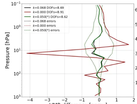
Figure 2. Differences between the fused profiles obtained with k=0.068 (black line),k=0 (red line) and the method used in Cec-cherini et al. (2018) (green line) (∗in this casekis applied to a CM built in a slightly different way; see text) and the mean of the true profiles related to the fusing profiles as a function of altitude (and pressure). The errors (dotted lines) and the numbers of DOFs of the three fused profiles are reported as well.

The use of simulated data makes it possible to compare the results with the true quantities that we want to measure. In Fig. 2, we report the differences between three fused profiles, obtained with k=0.068, with k=0 and with the method used in the previous paper on the importance of coincidence errors (Ceccherini et al., 2018), and the true profile of the fu-sion, calculated as the mean of the true profiles correspond-ing to the fuscorrespond-ing profiles. In the previous paper, an educated guess was made of the coincidence error andScoinequal to a matrix with the square of the 5 % of the a priori profile on the diagonal elements, and a correlation length of 6 km for the off-diagonal elements was used. In the figure, the errors and the numbers of DOFs of the three fused profiles are also reported.

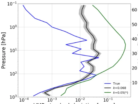
Figure 3.Square root of the diagonal elements ofScoinestimated

by the method described in Sect. 4.1 (black line), with its errors (grey band around the black line), and by the educated guess used in Ceccherini et al. (2018) (green line) (∗in this casekis applied to a CM built in a slightly different way; see text) as a function of altitude (and pressure) compared with the standard deviation of the true profiles corresponding to the fusing profiles (blue line).

In Fig. 3, we report the square root of the diagonal ele-ments ofScoinestimated by the method described in Sect. 4.1 (with its errors) and by the method used in the previous pa-per as a function of altitude (and pressure) and compare them with the standard deviation of the true profiles corresponding to the fusing profiles.

We see that the method described in Sect. 4.1 is able to reproduce the standard deviation of the true profiles well up to about 30 km of altitude. Above 30 km this method over-estimates the spread of the true profiles, likely because we assumeScoinproportional to the a priori CM, which includes the day–night variability of ozone. This variability is instead absent in the fusing profiles because they belong to a sin-gle geostationary image that is acquired in 1 h. The educated guess ofScoinsignificantly overestimates the standard devia-tion of the true profiles below 8 km and above 15 km of alti-tude.

Within the limits posed by the fact that a single parameter is used for the estimate of a CM, the coincidence error deter-mined with the constraint of the cost function is a very good representation of the real geographical variability, much bet-ter than that obtained with the educated guess (please note the logarithmic scale in Fig. 3), although the effect of this differ-ence on the fusion process is very small, given the negligible consequences of overestimates of the coincidence error. 4.2.3 Analysis of all fusion cells

In order to evaluate the performances of the method de-scribed in Sect. 4.1 we introduce a quantifierβ equal to the root of the square sum of the relative differences between the

fused profile and its true profile:

β= v u u t

n

X

i=1

_x

fi−xti xti

2

, (31)

wherexfi is the ith component of the fused profile, xti is theith component of the true profile of the fusion andnis the number of levels of the fused profile. We calculated this quantifier for all the fusion cells.

In Fig. 4, we show the scatter plots ofβ and of the num-ber of DOFs (panel a and panel b, respectively) of the fused profiles obtained with thekvalues determined by the method described in Sect. 4.1 as a function of the same quantities obtained withkequal to zero. The number of fusing profiles is reported in the colour scale. In the case ofβ, small values are preferred; in the case of number of DOFs, large values are preferred.

From Fig. 4 we see that for large values of the number of fusing profiles in general the method described in Sect. 4.1 determines a significant reduction ofβ with respect to the case ofk equal to zero, while the effect on the number of DOFs is negligible. In some cases for small values of the number of fusing profiles, we see that the use of the large value ofk, erroneously determined by the method for the in-sufficient statistics, causes a significant reduction of the num-ber of DOFs and sometimes also an increase inβ. A worse value ofβ is also obtained in a few cases for cells that do not have a very small number of fusing profiles; however the loss observed in these cases is much smaller than the gain obtained in the much more numerous cells for which a re-duction ofβ is observed. The distribution of the colours in Fig. 4b clearly shows that the number of DOFs increases when the number of fusing profiles increases, confirming the improvement of information obtained with the fusion of many profiles.

A complete evaluation of the performances of the method has to take into account both the ability to reproduce the true profile (represented byβ) and the number of DOFs. For this reason, we define a new quantifierγ, equal to the ratio be-tweenβand the number of DOFs, which takes into account both aspects:

γ= β

DOFs. (32)

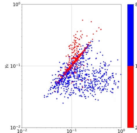
The quality of the fused profile improves when the value ofγ is reduced. In Fig. 5, we show the scatter plot ofγ of the fused profiles obtained with thekvalues determined by the method described in Sect. 4.1 as a function ofγ of the fused profiles obtained withkequal to zero. If the number of fusing profiles is smaller than 10 the points are reported in red, otherwise they are in blue.

Figure 4. (a)Scatter plot ofβkas a function ofβ0. The quantifier

βkcorresponds to thekvalue determined by the method described

in Sect. 4.1 and is reported on theyaxis, whileβ₀corresponds tok equal to zero and is reported on thexaxis.(b)Scatter plot of DOFsk

as a function of DOFs0. DOFskis the number of DOFs of the fused

profile obtained whenkis determined by the method described in Sect. 4.1 and is reported on theyaxis, while DOFs0is the number

of DOFs of the fused profile obtained whenkis equal to zero and is reported on thexaxis. The number of fusing profiles is reported in the colour scale.

of the fused profiles. Occasionally a worsening is observed, but improvements, in number and in entity, are overwhelm-ingly larger than worsenings. When the number of fusing profiles is smaller than 10 the k values determined by the method are affected by large errors (see Fig. 1) and values that are much larger than a reasonable expectation may be obtained. Therefore, it is not a surprise that in these cases the dominant effect is a degradation of the quality of the fused profiles with respect to the case ofkequal to zero. For this reason, the method described in Sect. 4.1 can only be used when eitherkis determined with a small error or, similarly, the number of fusing profiles is sufficiently large. In the other cases, an educated guess should be used, possibly supported by the indications provided by the results obtained in the cells with a large number of measurements.

5 Conclusions

The measurements that we wish to fuse often have some inconsistencies due to representations on different vertical grids, imperfect time and space coincidence, and different forward model errors. In order to apply the CDF method to inconsistent measurements it is necessary to add to the mea-surement CM of each fusing profile a CM that qualifies these inconsistencies as errors and prevents their use as erroneous features of the profile. Therefore, a realistic estimate of the inconsistency CM is required for effectual fused products. In this paper, we propose using the statistical properties of the cost function distribution to improve the estimate of the in-consistency CM.

The expected value and the variance of the cost function distribution of the data fusion have been analytically deter-mined for the first time. This allowed us to calculate the

re-Figure 5.Scatter plot ofγk as a function ofγ0. The quantifierγk

corresponds to thekvalue determined by the method described in Sect. 4.1 and is reported on theyaxis, whileγ0corresponds tok

equal to zero and is reported on thexaxis. If the number of fusing profiles is smaller than 10 the points are reported in red, otherwise they are in blue.

duced cost function, which is bound to be equal to 1 within the variability determined by its variance. Modelling the in-consistency CM with one parameter, we used the expected value of the reduced cost function as a constraint to tune the value of this parameter and the variance of the reduced cost function to assign an error to this value.

We applied this method to simulated measurements of ozone profiles obtained in the thermal infrared in the frame-work of the Sentinel-4 mission of the Copernicus pro-gramme. The results show that when the number of fusing profiles is small the values of the parameter are affected by large errors; in particular they are almost completely unde-termined if the number of fusing profiles is smaller than 10. For such small values of the number of fusing profiles, the method is not able to provide reliable values of the parame-ter and it is betparame-ter to use an educated guess for the estimate of the inconsistency CM. Conversely, when the number of fus-ing profiles is large enough the values of the parameter pro-vided by the method are affected by small errors and the esti-mated coincidence CMs generally improve the performances of the CDF method, providing a significant reduction of the differences between retrieved profile and true profile, with a negligible reduction of the number of DOFs.

Appendix A

In this appendix we make the calculation of the variance of the cost function given in Eq. (24).

The variance is equal to

varhcmin(σi)

i =

h

cmin(σi)−

D

cmin(σi)

Ei2

. (A1)

Substituting in Eq. (A1) the expression ofcmin(σi)given by Eq. (17), we obtain

varhcmin(σi)

i

=Dhcmin₀ +cmin₁ (σi)+cmin2 (σi)

−Dcmin₀ E−Dcmin₁ (σi)

E

−Dcmin₂ (σi)

Ei2

= _h

cmin₁ (σi)+c2min(σi)−

D

cmin₂ (σi)

Ei2

=

h

cmin₁ (σi)

i2 +

h

cmin₂ (σi)

i2

−Dcmin₂ (σi)

E2

, (A2)

where we used hcmin₀ i =c₀min, hcmin₁ (σ_i)i =0 and hc₁min(σ_i)c₂min(σ_i)i =0 because the product cmin₁ (σi)c₂min(σi) is cubic in the errors and, therefore, its expected value is zero as a consequence of the symmetry of the normal distribution.

Using Eq. (19), for the first term of Eq. (A2) we obtain

h

c₁min(σi)

i2

=4DσT_fS−_a1(xt−xa) (xt−xa)TS−a1σf

E

=4trhSfS−a1(xt−xa) (xt−xa)TS−a1

i

=4trh(xt−xa) (xt−xa)TS−a1Af(I−Af)

i

, (A3)

where we have used the relation SfS−a1=Af(I−Af) that comes from Eqs. (6) and (7).

Using Eq. (20), for the second term of Eq. (A2) we obtain

_h

c₂min(σi)

i2 =

*"_N X

i=1

σT_iS−_i 1σi

#2+

+

h

σT_f F+S−_a1σf

i2

−2

*"_N X

i=1

σT_iS−_i 1σiσTf

F+S−_a1σf

#2+

. (A4)

Some further elaboration is needed to evaluate these three terms:

*" _N X

i=1

σT_iS−_i1σi

#2+ =

N

X

i=1

D

σT_iS−_i 1σiσTiS −1 i σi

E

+

N

X

i,k=1, i6=k

D

σT_iS−_i 1σi

E D

σT_kS−_k1σk

E

=2

N

X

i=1

trS−_i 1SiS−_i 1Si

+

N

X

i=1

h

trS−_i 1Si

i2 +

N

X

i,k=1,i6=k

trSiS−i 1

trSkS−k1

=2

N

X

i=1 ni+

N

X

i,k=1 nink=

N

X

i=1 ni 2+

N

X

k=1 nk

!

, (A5)

_h

σT_fF+S−_a1σf

i2

=2trhF+S−_a1Sf

F+S−_a1Sf

i

+ntrhF+S−_a1Sf

io2

=2trA2_f+[tr(Af)]2 (A6) and

−2

*" _N X

i=1

σT_iS−_i 1σiσTf

F+S−_a1σf

#2+

= −2

N

X

i=1

σT_iS−_i 1σiσTiS −1 i Ai

F+S−_a1 −1

AT_iS−_i 1σi

−2

N

X

i,k=1, i6=k

D

σT_iS−_i 1σi

E

σT_kS−_k1AkF+S−_a1 −1

AT_kS−_k1σk

= −2

N

X

i=1 2tr

S−_i 1Ai

F+S−_a1 −1

AT_i

−2

N

X

i=1

trS−_i 1Si

tr

S−_i 1Ai

F+S−_a1 −1

AT_i

−2

N

X

i,k=1, i6=k

trS−_i 1Si

tr

S−_k1Ak

F+S−_a1 −1

AT_k

= −2tr(Af) 2+ N

X

i=1 ni

!

, (A7)

where we have used the formula for the expected value of the quartic form given in Petersen and Pedersen (2012), Eqs. (5)– (7) and Eq. (15).

The third term of Eq. (A2) is given by Eq. (22).

From Eq. (A2), using Eq. (22) and Eqs. (A3)–(A7), we obtain the expression of the variance of the cost function:

varhcmin(σi)

i

=2

N

X

i=1

ni−4tr(Af)+2tr

A2_f

+4trh(xt−xa) (xt−xa)TS−a1Af(I−Af)

i

Author contributions. SC calculated the expected value and the variance of the cost function and wrote the draft version of the pa-per. NZ wrote the Python code of the complete data fusion and ap-plied the procedure to determine the coincidence covariance matrix to the ozone simulated measurements. BC suggested the idea to use the cost function to determine the inconsistency covariance matrices and contributed to the interpretation of the results. SDB performed the simulation of the ozone measurements. UC and CT are, respec-tively, the principal investigator and the project manager of the AU-RORA project and coordinated the activity of the project. All the authors revised the paper.

Competing interests. The authors declare that they have no conflict of interest.

Acknowledgements. The results presented in this paper arise from research activities conducted in the framework of the AURORA project (http://www.aurora-copernicus.eu/, last access: 21 May 2019) supported by the Horizon 2020 research and inno-vation programme of the European Union (call: H2020-EO-2015; topic: EO-2-2015) under grant agreement no. 687428.

Financial support. This research has been supported by the Euro-pean Commission, H2020 (AURORA, grant no. 687428).

Review statement. This paper was edited by Andre Butz and re-viewed by two anonymous referees.

References

Aires, F., Aznay, O., Prigent, C., Paul, M., and Bernardo, F.: Syner-gistic multi-wavelength remote sensing versus a posteriori com-bination of retrieved products: Application for the retrieval of atmospheric profiles using MetOp-A, J. Geophys. Res., 117, D18304, https://doi.org/10.1029/2011JD017188, 2012. Calisesi, Y., Soebijanta, V. T., and Oss, R. V.:

Regrid-ding of remote sounRegrid-dings: formulation and application to ozone profile comparison, J. Geophys. Res., 110, D23306, https://doi.org/10.1029/2005JD006122, 2005.

Ceccherini, S.: Equivalence of measurement space solution data fu-sion and complete fufu-sion, J. Quant. Spectrosc. Ra., 182, 71–74, 2016.

Ceccherini, S. and Ridolfi, M.: Technical Note: Variance-covariance matrix and averaging kernels for the Levenberg-Marquardt so-lution of the retrieval of atmospheric vertical profiles, Atmos. Chem. Phys., 10, 3131–3139, https://doi.org/10.5194/acp-10-3131-2010, 2010.

Ceccherini, S., Carli, B., Pascale, E., Prosperi, M., Raspollini, P., and Dinelli, B. M.: Comparison of measurements made with two different instruments of the same atmospheric vertical profile, Appl. Opt., 42, 6465–6473, 2003.

Ceccherini, S., Raspollini, P., and Carli, B.: Optimal use of the infor-mation provided by indirect measurements of atmospheric verti-cal profiles, Opt. Express., 17, 4944–4958, 2009.

Ceccherini, S., Carli, B., Cortesi, U., Del Bianco, S., and Raspollini, P.: Retrieval of the vertical column of an atmospheric constituent from data fusion of remote sensing measurements, J. Quant. Spectrosc. Ra., 111, 507–514, 2010a.

Ceccherini, S., Cortesi, U., Del Bianco, S., Raspollini, P., and Carli, B.: IASI-METOP and MIPAS-ENVISAT data fusion, At-mos. Chem. Phys., 10, 4689–4698, https://doi.org/10.5194/acp-10-4689-2010, 2010b.

Ceccherini, S., Carli, B., and Raspollini, P.: Quality quantifier of indirect measurements, Opt. Express, 20, 5151–5167, 2012. Ceccherini, S., Carli, B., and Raspollini, P.: Equivalence of data

fu-sion and simultaneous retrieval, Opt. Express, 23, 8476–8488, 2015.

Ceccherini, S., Carli, B., and Raspollini, P.: Vertical grid of retrieved atmospheric profiles, J. Quant. Spectrosc. Ra., 174, 7–13, 2016. Ceccherini, S., Carli, B., Tirelli, C., Zoppetti, N., Del Bianco,

S., Cortesi, U., Kujanpää, J., and Dragani, R.: Importance of interpolation and coincidence errors in data fusion, Atmos. Meas. Tech., 11, 1009–1017, https://doi.org/10.5194/amt-11-1009-2018, 2018.

Cortesi, U., Del Bianco, S., Ceccherini, S., Gai, M., Dinelli, B. M., Castelli, E., Oelhaf, H., Woiwode, W., Höpfner, M., and Gerber, D.: Synergy between middle infrared and millimeter-wave limb sounding of atmospheric temperature and minor constituents, At-mos. Meas. Tech., 9, 2267–2289, https://doi.org/10.5194/amt-9-2267-2016, 2016.

Cortesi, U., Ceccherini, S., Del Bianco, S., Gai, M., Tirelli, C., Zoppetti, N., Barbara, F., Bonazountas, M., Argyridis, A., Bós, A., Loenen, E., Arola, A., Kujanpää, J., Lipponen, A., Nyamsi, W. W., van der A, R., van Peet, J., Tuinder, O., Farruggia, V., Masini, A., Simeone, E., Dragani, R., Keppens, A., Lambert, J.-C., van Roozendael, M., Lerot, J.-C., Yu, H., and Verberne, K.: Advanced Ultraviolet Radiation and Ozone Retrieval for Appli-cations (AURORA): A Project Overview, Atmosphere, 9, 454, https://doi.org/10.3390/atmos9110454, 2018.

ESA: Sentinel-4: ESA’s Geostationary Atmospheric Mission for Copernicus Operational Services, SP1334, April 2017, avail-able at: http://esamultimedia.esa.int/multimedia/publications/ SP-1334/SP-1334.pdf (last access: 21 May 2019), 2017. Fisher, R. A.: The logic of inductive inference, J. Roy. Stat. Soc.,

98, 39–54, 1935.

Gelaro, R., McCarty, W., Max, J., Suárez, M. J., Todling, R., Molod, A., Takacs, L., Randles, C. A., Darmenov, A., Bosilovich, M. G., Reichle, R., Wargan, K., Coy, L., Cullather, R., Draper, C., Akella, S., Buchard, V., Conaty, A., da Silva, A. M., Gu, W., Kim, G. K., Koster, R., Lucchesi, R., Merkova, D., Nielsen, J. E., Par-tyka, G., Pawson, S., Putman, W., Rienecker, M., Schubert, S. D., Sienkiewicz, M., and Zhao, B.: The Modern-Era Retrospective Analysis for Research and Applications, Version 2 (MERRA-2), J. Climate, 30, 5419–5454, https://doi.org/10.1175/JCLI-D-16-0758.1, 2017.

Kroon, M., de Haan, J. F., Veefkind, J. P., Froidevaux, L., Wang, R., Kivi, R., and Hakkarainen, J. J.: Validation of operational ozone profiles from the Ozone Monitoring Instrument, J. Geophys. Res., 116, D18305, https://doi.org/10.1029/2010JD015100, 2011.

Liu, X., Bhartia, P. K., Chance, K., Spurr, R. J. D., and Kurosu, T. P.: Ozone profile retrievals from the Ozone Mon-itoring Instrument, Atmos. Chem. Phys., 10, 2521–2537, https://doi.org/10.5194/acp-10-2521-2010, 2010.

McPeters, R. D. and Labow, G. J.: Climatology 2011: An MLS and sonde derived ozone climatology for satel-lite retrieval algorithms, J. Geophys. Res., 117, D10303, https://doi.org/10.1029/2011JD017006, 2012.

Miles, G. M., Siddans, R., Kerridge, B. J., Latter, B. G., and Richards, N. A. D.: Tropospheric ozone and ozone profiles re-trieved from GOME-2 and their validation, Atmos. Meas. Tech., 8, 385–398, https://doi.org/10.5194/amt-8-385-2015, 2015.

Petersen, K. B. and Pedersen, M. S.: The matrix cook-book, available at: https://www.math.uwaterloo.ca/~hwolkowi/ matrixcookbook.pdf (last access: 21 May 2019), 2012.

Quesada-Ruiz, S., Attié, J.-L., Lahoz, W. A., Abida, R., Ricaud, P., El Amraoui, L., Zbinden, R., Piacentini, A., Joly, M., Eskes, H., Segers, A., Curier, L., de Haan, J., Kujanpää, J., Oude-Nijhuis, A., Tamminen, J., Timmermans, R., and Veefkind, P.: Benefit of ozone observations from Sentinel-5P and future Sentinel-4 mis-sions on tropospheric composition, Atmos. Meas. Tech. Discuss., https://doi.org/10.5194/amt-2018-456, in review, 2019. Rodgers, C. D.: Inverse Methods for Atmospheric Sounding: