https://doi.org/10.5194/os-15-967-2019
© Author(s) 2019. This work is distributed under the Creative Commons Attribution 4.0 License.
Skill assessment of global, regional, and coastal circulation
forecast models: evaluating the benefits of dynamical
downscaling in IBI (Iberia–Biscay–Ireland) surface waters
Pablo Lorente1,2, Marcos García-Sotillo2, Arancha Amo-Baladrón1,2, Roland Aznar1,2, Bruno Levier3, José C. Sánchez-Garrido4, Simone Sammartino4, Álvaro de Pascual-Collar1,2, Guillaume Reffray3, Cristina Toledano1,2, and Enrique Álvarez-Fanjul2
1Nologin Consulting S.L., Zaragoza, 50018, Spain 2Puertos del Estado, Madrid, 28042, Spain 3Mercator Ocean, Toulouse, 31520, France
4Physical Oceanography Group of University of Málaga, Málaga, 29071, Spain
Correspondence:Pablo Lorente ([email protected])
Received: 31 December 2018 – Discussion started: 17 January 2019 Revised: 19 June 2019 – Accepted: 25 June 2019 – Published: 22 July 2019
Abstract. In this work, a multi-parameter inter-comparison of diverse ocean forecast models was conducted at the sea surface ranging from global to local scales in a two-phase stepwise strategy. Firstly, a comparison of CMEMS GLOBAL and the nested CMEMS IBI regional system was performed against satellite-derived and in situ observations. Results highlighted the overall benefits of both the GLOBAL direct data assimilation in open water and the increased hori-zontal resolution of IBI in coastal areas. Besides, IBI (Iberia– Biscay–Ireland) proved to capture shelf dynamics by bet-ter representing the horizontal extent and strength of a river freshwater plume, according to the results derived from the validation against in situ observations from a buoy moored in NW Spain. Secondly, a multi-model inter-comparison exer-cise for 2017 was performed in the Strait of Gibraltar among GLOBAL, IBI, and SAMPA (Sánchez-Garrido et al., 2013) high-resolution coastal forecast systems (partially nested to IBI) in order to elucidate the accuracy of each system to char-acterize the Atlantic Jet (AJ) inflow dynamics. A quantita-tive validation against hourly currents from high-frequency radar (HFR) highlighted both the steady improvement in AJ representation in terms of speed and direction when zoom-ing from global to coastal scales through a multi-nestzoom-ing model approach and also the relevance of a variety of fac-tors at local scale such as a refined horizontal resolution, a tailored bathymetry, and a higher spatio-temporal resolu-tion of the atmospheric forcing. The ability of each model
to reproduce a 2 d quasi-permanent full reversal of the AJ surface inflow was examined in terms of wind-induced cir-culation patterns. SAMPA appeared to better reproduce the reversal events detected with HFR estimations, demonstrat-ing the added value of imposdemonstrat-ing accurate meteorologically driven barotropic velocities in the open boundaries (imported from the NIVMAR (Álvarez-Fanjul et al., 2001) storm surge model) to take into account the remote effect of the atmo-spheric forcing over the entire Mediterranean basin, which was only partially included in IBI and GLOBAL systems. Fi-nally, SAMPA coastal model outputs were also qualitatively analysed in the western Alboran Sea to put in a broader per-spective the context of the onset, development, and end of such flow reversal episodes.
1 Introduction
in order to reliably portray and predict the ocean state and its variability at diverse spatio-temporal scales.
Global circulation models have been steadily evolving in terms of complexity, horizontal resolution refinement, and process parameterization (Holt et al., 2017). Notwithstand-ing, such development involves compromises of scale and is subject to practical limits on the feasible spatial resolu-tion (Greenberg et al., 2007). Although large-scale physical processes are properly resolved by the current state-of-the-art global model resolution (e.g. nominal 1/12◦), coastal and shelf phenomena are still poorly replicated or even misrepre-sented as the grid mesh is too coarse. This is especially true for complex-geometry regions such as sea straits, archipela-gos, or semi-enclosed seas where the coastline, seamounts, and bottom topography are not well resolved. In this context, tides, vertical coordinates, mixing schemes, river inflows, and atmospheric forcings have been traditionally identified as five areas of further research in global ocean modelling (Holt et al., 2017).
Since the continental shelf is affected not only by natu-ral agents (land–sea breezes, riverine discharges, bottom to-pography, coastline shape, etc.) but also by human-induced factors, an increased understanding of coastal circulation is essential for decision- and policy-making in the socioeco-nomically vital and often environmentally stressed coastal regions. Therefore, small-scale ocean features must be ex-plicitly computed and accurately reproduced by means of re-gional models with finer horizontal grid spacing but for a particular delimited area. The success of this approach re-quires the seamless progress in several aspects, as previ-ously identified by Wilkin et al. (2017) and Kourafalou et al. (2015): (i) a deep comprehension of the primary mech-anisms driving coastal circulation, (ii) downscaling meth-ods to adequately represent air–sea and land–sea interactions, and (iii) robust methods to embed high-resolution models in coarser-scale systems. Therefore, this approach implies the transfer of large-scale information from the global model to the interior of the nested regional domain by means of diverse methodologies. One of them is the so-called “spectral nudg-ing” technique, adopted to ensure that the prevailing global conditions are not degraded in the open ocean, while allow-ing submesoscale processes to be resolved exclusively by the nested model in the continental shelf and coastal areas (Her-bert et al., 2014). An alternative approach to computational time-demanding multiple nesting procedures consists of us-ing unique unstructured grid models as they have proved to properly describe ocean processes at different spatial scales (Ferrarin et al., 2013, 2019; Federico et al., 2017; Cucco et al., 2012). They benefit from imposing higher resolution in shallow water areas to better resolve irregular coastlines, in-tricate bathymetries, and hence small-scale dynamics while applying a coarser grid resolution in open water to reproduce large-scale phenomena. Besides, unstructured grid models are particularly effective to achieve the seamless transition
between adjoining basins interconnected by narrow straits (Ferrarin et al., 2018; Stanev et al., 2017; Zhang et al., 2016). Additionally, the regional modelling strategy can include some fine-tuning of physical parameters, individually tai-lored to each chosen area, instead of the universally valid parameterizations associated with global OOFSs. The ben-efits of regional modelling over the driving global OOFS are generally assumed but to date only few studies have explored and quantified the potential added value of such approaches (Katavouta and Thomson, 2016; Rockel, 2015; Greenberg et al., 2007). The “parent–son” model inter-comparison is mandatory during both implementation and operational stages since it aids to (i) verify the most ade-quate nesting strategy, (ii) check the consistency of the nested model solution, and (iii) identify any potential problem that might be inherited from the coarser system.
In the framework of the Copernicus Marine Environment Monitoring Service (CMEMS), a global ocean model to-gether with a wealth of nested regional OOFSs are currently running in different areas of the European seas and providing paramount oceanographic forecast products (Le Traon et al., 2018). Since the validation of OOFSs against independent measurements constitutes a core activity in oceanographic operational centres, the skill of Iberia–Biscay–Ireland (IBI) regional OOFS is routinely assessed by means of the NAR-VAL (North Atlantic Regional NAR-VALidation) system (Sotillo et al., 2015), a web-based toolbox that provides a series of skill metrics automatically computed and delivered in the QUality Information Document – QUID – (Sotillo et al., 2018). In this context, the first goal of this paper is to con-duct a multi-parameter model inter-comparison between IBI regional OOFS and the coarser parent system, the CMEMS GLOBAL (Lellouche et al., 2018), with the aim of assessing their performance at the upper ocean layer. Their predictive skills to properly represent the sea surface temperature (SST) over IBI coverage domain and diverse subregions were eval-uated by means of comparisons against remote-sensed and in situ observations. On the other hand, their prognostic capa-bilities to accurately reproduce the coastal surface circulation were assessed through the analysis of a single impulsive-type river outflow episode that took place in March 2018 in the Galician coast (NW Spain), a region of freshwater influence – ROFI – (Simpson, 1997).
sys-tems (Lin et al., 2008; Pérez et al., 2013). By contrast, less attention has been devoted to hydrodynamic harbour condi-tions since its reduced dimensions and intricate layout con-fer harbour restrictions which are not present in the open sea. Besides, derivative products based on current forecasts, such as float trajectories, residence time maps, flushing pat-terns, and risk assessment of water quality degradation, can constitute additional assets for efficient harbour management (Álvarez-Fanjul et al., 2018; Sammartino et al., 2018). In or-der to overcome the existing gap between the scales effec-tively solved by the regional OOFSs and the coastal scales required to meet strong societal needs in support of blue and green growth, a number of downstream services are currently adopting different downscaling approaches. Dy-namical downscaling takes regional boundary conditions to drive a high-resolution limited-area model in which coastal processes are calculated on a finer grid by resolving well-known hydrodynamic equations. However, uncertainties in the downscaling process must be evaluated since coastal model performance can be directly impacted by the prop-agation of any potential issue in the large-scale dynamics, inherited from the coarser system (Hernández et al., 2018).
As a representative example of downstream service de-veloped by Puertos del Estado (PdE) in a hot spot area like the Strait of Gibraltar (GIBST), the operational PdE-SAMPA high-resolution coastal system (Sánchez-Garrido et al., 2013) is partially embedded in IBI and nowadays em-ployed by the Port Authority of Algeciras Bay as predic-tive tool to support maritime policy and assist with high-risk decision-making related to marine safety, port operation optimization, and mitigation of both natural disasters and anthropogenic hazards. Previous research has unequivocally proved the ability of PdE-SAMPA to accurately capture ba-sic circulation features of the GIBST area and Algeciras Bay (Sanchez-Garrido et al., 2014; Sammartino et al., 2014; Soto-Navarro et al., 2016). A preliminary model skill assessment was conducted within the framework of the MEDESS-4MS project (Sotillo et al., 2016a). However, the added value of this coastal OOFS with respect to the regional IBI system was only quantified from a Lagrangian perspective by us-ing a wealth of drifters. The second goal of this contribu-tion is thus to build upon previous model inter-comparison exercises, placing special emphasis on the characterization of the Atlantic Jet (AJ) inflow into the Mediterranean Sea in terms of speed and direction. This geostrophically ad-justed jet fluctuates on a wide range of temporal scales and drives the main circulation in the Alboran Sea, feeding and surrounding the Western Alboran Gyre – WAG – (Macias et al., 2016). An inter-comparison exercise was conducted for 2017 among a global configuration (CMEMS GLOBAL), a regional application (CMEMS IBI) and a higher resolu-tion coastal system (PdE-SAMPA) in order to characterize the AJ dynamics and their ability to adequately capture an extreme event: the quasi-permanent (up to∼48 h long) full reversal of the AJ surface flow under intense and prolonged
easterlies. To this end, a high-frequency radar (HFR) has been used as benchmark since it regularly provides quality-controlled hourly maps of the surface currents of the strait (Lorente et al., 2014). A detailed characterization of this un-usual phenomenon is relevant from diverse aspects, encom-passing search and rescue operations (to adequately expand westwards the search area), the management of accidental marine pollution episodes (to establish alternative contin-gency plans), or safe ship routing (to maximize fuel effi-ciency).
In summary, this paper serves one primary purpose: per-forming a multi-parameter model skill assessment in IBI sur-face waters, ranging from global to local scales in a two-phase stepwise strategy. This includes (i) a comparison be-tween GLOBAL and IBI regional systems in the entire over-lapping coverage domain, focusing special attention on re-gionalization and (ii) an event-oriented multi-model inter-comparison for 2017 with a focus on the complete inversion of the surface flow in the GIBST. This process-based vali-dation approach, albeit commonly used in meteorology and weather forecasting, is rather novel in operational oceanogra-phy and mostly devoted to extreme sea level and wave height episodes.
This paper is organized as follows: Sect. 2 provides fur-ther details about the study areas, Sect. 3 describes the di-verse models configuration, Sect. 4 outlines the observational data sources and methodology used in this study, and Sects. 5 and 6 present a detailed discussion of the results. Finally, main conclusions are summarized in Sect. 7.
2 Study areas
2.1 IBI area (and subregions)
Shelf and coastal areas of the region are also affected by strong storm surges (Pérez et al., 2012). Along the western Iberian and African coasts, strong summer upwelling of bot-tom cold and enriched waters takes place under predominant northerly wind conditions that trigger the Ekman-driven off-shore deflection of the surface flux.
IBI is also a rather broad and heterogeneous area. In or-der to gain insight into the model skill assessment (as later explained in Sect. 5), the IBI service (IBISR) regional do-main has been split into nine different subregions (Fig. 1a): the Irish Sea (IRISH), the English Channel (ECHAN), the Gulf of Biscay (GOBIS), the North Iberian Shelf (NIBSH), the West Iberian Shelf (WIBSH), the Western Mediterranean Sea (WSMED), the Gulf of Cádiz (CADIZ), the Strait of Gibraltar (GIBST), and the Canary Islands (ICANA).
2.2 Strait of Gibraltar
The Strait of Gibraltar (GIBST), the only connection be-tween the semi-enclosed Mediterranean basin and the open Atlantic Ocean (Fig. 1b), is characterized by a two-layer baroclinic exchange which is hydraulically controlled at Ca-marinal Sill (Sánchez-Garrido et al., 2011). Whilst saltier Mediterranean water flows out at depth, an eastward surface jet of relatively fresh Atlantic water (AJ) flows into the Alb-oran Sea by surrounding the quasi-permanent Western An-ticyclonic Gyre (WAG) and the more elusive Eastern Anti-cyclonic Gyre (EAG) in a wavelike path. As the WAG owes its existence to the input of new Atlantic waters provided by the AJ, both structures are widely considered to be coupled and usually referred to as the AJ–WAG system. A significant variety of analytical, field, and modelling studies have pre-viously attempted to disentangle the AJ–WAG system and properly explain the underlying physical processes (Sánchez-Garrido et al., 2013; Macías et al., 2007a; Viúdez, 1997).
The position, intensity, and direction of the AJ fluctuate on a broad range of temporal scales, driving the upper-layer circulation of the Alboran Sea with subsequent physical and biological implications (Solé et al., 2016; Sánchez-Garrido et al., 2015; Ruiz et al., 2013). For instance, the presence of a strong AJ close to the northern shore of the Alboran Sea reinforces the coastal upwelling and therefore increases both the near-shore chlorophyll concentration and the spawning of fish in this region (Ruiz et al., 2013; Macías et al., 2008). By contrast, meteorologically induced inflow interruptions can trigger weakening and even the decoupling of the AJ– WAG system (Sánchez-Garrido et al., 2013), the subsequent eastward migration of the WAG, and the genesis of a new gyre that coexists with the other two, giving rise to a three-anticyclonic-gyre situation (Viúdez et al., 1998).
Within this context, the AJ pattern has been described to oscillate between two main circulation modes at seasonal scale (Vargas-Yáñez et al., 2002): (i) a stronger AJ flows northeastwards during the first half of the year and (ii) a weaker AJ flows more southwardly towards the end of the
year. Sea level pressure (SLP) variations over the western Mediterranean basin and local zonal wind (U) fluctuations in the Alboran Sea are usually considered the main factors controlling and modulating the AJ variability (Macías et al., 2007b; García-Lafuente et al., 2002a, b). In particular, the second parameter has been largely invoked as the primary driving agent to explain both the intensification of the surface inflow during prevalent westerlies and also extreme AJ col-lapse events recorded when intense easterlies are predomi-nant (Macías et al., 2016). The zonal wind intensity has been reported to follow an annual cycle with more westerly (east-erly) winds during winter (summer) months (Dorman et al., 1995). The seasonal variability and occasional interruptions of the Atlantic inflow due to meteorological forcing have been earlier investigated with in situ data from fixed moor-ings (García-Lafuente et al., 2002a). More recently, a consid-erable number of satellite-tracked drifters were released on both sides of GIBST within the framework of the MEDESS-4MS project, hence providing a complete Lagrangian view of the Atlantic water inflow into the Alboran Sea (Sotillo et al., 2016-b).
3 Model descriptions
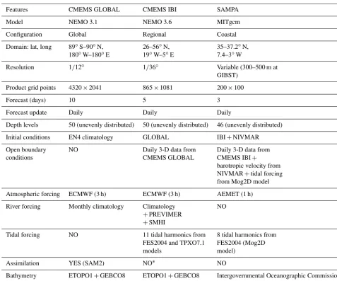
Whereas basic features of the three OOFSs employed in this work are gathered in Table 1, further details are provided in the following devoted subsections.
3.1 CMEMS GLOBAL system
The operational mercator global ocean analysis and forecast system provides 10 d of 3-D global ocean forecasts updated daily. This product includes daily mean files of temperature, salinity, currents, sea level, mixed layer depth, and ice pa-rameters from the surface to seafloor over the global ocean. It also includes hourly mean surface fields for sea level height, temperature, and currents. The global ocean output files are displayed with a 1/12◦horizontal resolution with regular lat-itude and longlat-itude equirectangular projection. Some 50 ver-tical levels span from 0 to 5500 m.
Figure 1. (a) Iberia–Biscay–Ireland service (IBISR) domain, which comprises nine subregions denoted by red squares. Filled red dots represent buoy locations.(b)Study area: coverage domain of SAMPA coastal ocean model, where the surface Atlantic Jet (AJ) flows through the Strait of Gibraltar into the Alboran Sea, feeding the Western Alboran Gyre (WAG); isobath depths are labelled every 200 m. Red dots indicate a topographic feature: Camarinal Sill (CS).(c)HFR hourly data availability for 2017: solid black squares represent radar sites, blue and red dots indicate Tarifa tide gauge and B7 buoy location, respectively. The black line denotes the selected transect and the white square represents its midpoint.
further details, the reader is referred to the GLOBAL Product User Manual – PUM – (Law Chune et al., 2019).
The system is based on the Nucleus for European Mod-elling of the Ocean (NEMO) v3.1 ocean model (Madec, 2008). The physical configuration is based on the tripolar ORCA (Madec and Imbard, 1996) grid type with a hor-izontal resolution of 9 km at the Equator, 7 km at Cape Hatteras (mid-latitudes), and 2 km towards the Ross and Weddell seas. The 50-level vertical discretization retained for this system has 1 m resolution at the surface decreas-ing to 450 m at the bottom, and 22 levels within the upper 100 m. The bathymetry used in the system is a combina-tion of interpolated ETOPO1 (Earth TOPOgraphy 1 arcmin) and GEBCO8 (GEneral Bathymetric Chart of the Oceans, version 8) databases. The system was initialized on 11 Oc-tober 2006 based on the temperature and salinity profiles from the EN4 monthly gridded climatology. The atmospheric fields forcing the ocean model are taken from the ECMWF (European Centre for Medium-Range Weather Forecasts) In-tegrated Forecast System. A 3 h sampling is used to repro-duce the diurnal cycle. The system does not include tides nor pressure forcing. The monthly runoff climatology is built with data on coastal runoffs and 100 major rivers from the Dai et al. (2009) database (Lellouche et al., 2018). Altime-ter data, in situ temperature and salinity vertical profiles, and satellite sea surface temperature data are jointly assimilated to estimate the initial conditions for numerical ocean fore-casting. Moreover, satellite sea ice concentration data are now assimilated in the system in a variate or
mono-data mode. More information can be found in Lellouche et al. (2018).
3.2 CMEMS IBI regional system
The IBI OOFS provides a real-time short-term 5 d hydrody-namic 3-D forecast (and 1 d of hindcast as best estimate) of a range of physical parameters (currents, temperature, salin-ity, and sea level) since 2011 (Sotillo et al., 2015). IBI is based on an eddy-resolving NEMO model application (v3.6) that includes high-frequency processes required to character-ize regional-scale marine processes. The model application is run at 1/36◦ horizontal resolution and final products are routinely delivered in a service domain extending between 26–56◦N and 19◦W–5◦E. The NEMO model (Madec, 2008) solves the three-dimensional finite-difference primitive equa-tions in spherical coordinates discretized on an Arakawa-C grid and 50 geopotential vertical levels (z coordinate), as-suming hydrostatic equilibrium and Boussinesq approxima-tion. Partial bottom cell representation of the bathymetry (a composite of ETOPO2 and GEBCO8) allows an accurate representation of the steep slopes characteristic of the area. The model grid is a subset of the Global 1/12◦ORCA tripo-lar grid used by the parent system (the CMEMS GLOBAL system) that provides initial and lateral boundary conditions (west – the Atlantic Ocean, east – the Western Mediterranean Sea), but refined at 1/36◦horizontal resolution.
rel-Table 1.Basic features of the ocean forecast systems employed in the present study.∗The operational version of IBI used with spectral nudging. Assimilation scheme SAM2 was later introduced in version 4 (April 2018).
Features CMEMS GLOBAL CMEMS IBI SAMPA
Model NEMO 3.1 NEMO 3.6 MITgcm
Configuration Global Regional Coastal
Domain: lat, long 89◦S–90◦N, 26–56◦N, 35–37.2◦N,
180◦W–180◦E 19◦W–5◦E 7.4–3◦W
Resolution 1/12◦ 1/36◦ Variable (300–500 m at
GIBST)
Product grid points 4320×2041 865×1081 200×100
Forecast (days) 10 5 3
Forecast update Daily Daily Daily
Depth levels 50 (unevenly distributed) 50 (unevenly distributed) 46 (unevenly distributed)
Initial conditions EN4 climatology GLOBAL IBI+NIVMAR
Open boundary NO Daily 3-D data from Daily 3-D data from
conditions CMEMS GLOBAL CMEMS IBI+
barotropic velocity from NIVMAR+tidal forcing from Mog2D model
Atmospheric forcing ECMWF (3 h) ECMWF (3 h) AEMET (1 h)
River forcing Monthly climatology Climatology NO
+PREVIMER
+SMHI
Tidal forcing NO 11 tidal harmonics from 8 tidal harmonics from
FES2004 and TPXO7.1 FES2004 (Mog2D
models model)
Assimilation YES (SAM2) NO∗ NO
Bathymetry ETOPO1+GEBCO8 ETOPO1+GEBCO8 Intergovernmental Oceanographic Commission
+high-resolution charts
ative humidity, precipitation, shortwave and longwave ra-diative fluxes) provided by ECMWF. CORE empirical bulk formulae (Large and Yeager, 2004) are used to compute la-tent sensible heat fluxes, evaporation, and surface stress. Lat-eral open boundary data are interpolated from the daily out-puts of the GLOBAL system. These are complemented by 11 tidal harmonics built from FES2004 (Lyard et al., 2006) and TPXO7.1 (Egbert and Erofeeva, 2002) tidal model solu-tions. Atmospheric pressure component, missing in the large-scale parent system sea level outputs, is included assuming pure isostatic response at open boundaries (inverse barometer approximation). Fresh water river discharge inputs are imple-mented as lateral open boundary condition for 33 rivers. Flow rate data imposed are based on a combination of daily ob-servations from PREVIMER, simulated data from E-HYPE hydrological model, and monthly climatological data from Global Runoff Data Centre (GDRC) and French “Banque
Hydro” datasets. Further details can be found in Sotillo et al. (2015).
Originally, the operational IBI system was based on a peri-odic reinitialization from the GLOBAL parent solution. Af-terwards, IBI has steadily evolved: by April 2016, an upgrade of the downscaling methodology was implemented, substi-tuting the periodic reinitialization by a spectral nudging tech-nique in order to avoid temporal discontinuity inherent to the periodic reinitialization and to minimize dependency from the GLOBAL parent solution on the shelf.
for a chosen state variable X (typically currents, tempera-ture, and salinity). Such an increment consists of a space and time low-pass filter of the differencesXp–Xcin order to keep the characteristic scales so the parent GLOBAL system can properly resolve (from large scale to mesoscale). After each forecast cycle of the child IBI system, a new cycle (called analysis) is relaunched where Xc is nudged toXp at each time step by the weekly mean of the daily increments previ-ously computed in the parent system grid during the forecast cycle. The 1-week time smoothing window was imposed as this is the typical timescale associated with mesoscale struc-tures.
Furthermore, the nudging is spatially limited in those areas where the parent system can not improve the regional model (e.g. where there is no data assimilation of altimetry or where the physics is missing, for instance on the shelf) or where the spatial filtering processes are potentially detrimental (close to the bottom or the open boundaries). This spatial weight function is a 3-D mask (for further details, see Herbert et al., 2014) that differentiates the zones where IBI system is nudged and thus reconciled with the parent system (typically in the open sea) from those where IBI remains free (continen-tal shelf, coas(continen-tal areas, and regions close to the open bound-aries) to fully compute higher-frequency processes such as thermal tidal fronts, river discharges, etc.
Finally, a SAM2-based data assimilation scheme (Lel-louche et al., 2013; Brasseur et al., 2005) was recently in-troduced (April 2018) in order to enhance IBI predictive skills but will not be further described here as only outputs from 2017 have been used in the present work.
3.3 PdE SAMPA coastal system
The PdE-SAMPA operational forecast service started in April 2012 (Sammartino et al., 2014; Sánchez-Garrido et al., 2014). It routinely provides a daily short-term forecast (72 h horizon) of currents and other oceanographic vari-ables in the Strait of Gibraltar and its surroundings (Gulf of Cádiz and Alboran Sea). The PdE-SAMPA model applica-tion was developed by the University of Málaga in collab-oration with PdE in order to provide a tailored forecasting service to one of their main stakeholders, the harbour of Al-geciras Bay (Fig. 1b). It is based on the Massachusetts In-stitute of Technology global circulation model – MITgcm – (Marshall et al., 1997). The domain, which extends from the Gulf of Cádiz to the Alboran Sea (Fig. 1b), is discretized with an orthonormal curvilinear grid of variable horizontal resolution, sparser close to the boundaries (∼8–10 km), and higher in the strait (∼300–500 m). In the vertical dimen-sion, SAMPA has 46 unevenly spaced zlevels with maxi-mum resolution of 5 m near the surface, exponentially de-caying towards the seafloor. The shallower level is at 2.5 m depth. The bathymetry is derived from a combination of the GEBCO bathymetry dataset and fine-resolution bathy-metric charts of the Strait of Gibraltar and the continental
shelf of the Gulf of Cádiz and northern coast of the Alb-oran Sea. The bottom topography is represented as partial vertical cells. In the two lateral open boundaries (west – the Atlantic Ocean, east – the Western Mediterranean Sea) the model is partially forced by daily mean temperature, salinity, and velocity fields from CMEMS IBI regional model (Sotillo et al., 2015). Since such frequency is not suitable to resolve barotropic flows through the strait either (García-Lafuente et al., 2002b), tidal and meteorologically driven barotropic ve-locities are prescribed across the open boundaries: the for-mer extracted from the Mog2D model described by Carrere and Lyard (2003) and the latter from the storm surge op-erational system developed by Álvarez-Fanjul et al. (2001), which accounts for the remote effect of the atmospheric forc-ing in the barotropic flow through GIBST. This nestforc-ing strat-egy ensures that the SAMPA model captures a realistic vari-ability in inflow and outflow currents through the strait. At the sea surface, the model is forced by hourly values of wind stress, air humidity and temperature, fresh water, and heat surface fluxes provided by the Spanish Meteorologi-cal Agency through the operational Forecast System based on the HIRLAM model (Cats and Wolters, 1996). Further details on the SAMPA model configuration are provided in Sanchez-Garrido et al. (2013).
4 Validation of OOFSs 4.1 Framework
The validation of OOFSs against independent measurements constitutes a core activity in oceanographic operational cen-tres since it aids (i) to infer the relative strengths and weak-nesses in the modelling of several key physical processes, (ii) to compare different versions of the same OOFS and eval-uate potential improvements and degradations before a new version is transitioned into operational status, (iii) to compare coarse-resolution “father” and nested high-resolution “son” systems to quantify the added value of downscaling.
spatio-temporal uncertainty levels. The evaluation metrics regularly generated by NARVAL are delivered online in the QUID, which is periodically updated and freely available on the CMEMS website (http://marine.copernicus.eu/, last ac-cess: 1 July 2019).
Complementarily, opportunistic inter-comparisons are conducted in the frame of diverse EU-funded projects such as MEDESS-4MS (Sotillo et al., 2016a): 35 satellite-tracked drifters were released on both sides of the Strait of Gibral-tar and the quality-controlled in situ data of sea surface tem-perature and currents were collected to build the MEDESS-GIB database (Sotillo et al., 2016b), hence providing a com-plete Lagrangian view of the surface inflow of Atlantic wa-ters through the GIBST and the Alboran Sea. Such valuable oceanographic information was subsequently used to com-pare IBI and SAMPA forecast products to identify strengths (realistic simulation of the Atlantic Jet and the Algerian Cur-rent) and shortcomings (position and intensity of the Albo-ran gyres, especially the western one) in both model perfor-mances. This exercise reflected the effectiveness of the dy-namical downscaling performed through the SAMPA system with respect to the regional solution (in which SAMPA is partially nested, as it is also embedded in Mog2D and NIV-MAR models), providing an objective measure of the poten-tial added value introduced by SAMPA.
Eventually, ancillary validation approaches have been re-cently adopted focused on the evaluation of ocean model per-formances in specific situations and on their ability to accu-rately reproduce singular oceanographic processes (Hernán-dez et al., 2018). Since the NARVAL tool is devoted to compare model solutions on a monthly, seasonal, or an-nual basis, part of the picture is missing due to traditional time averaging. Hence the quality indicators computed, al-beit valid, mask somehow model capabilities to replicate ocean phenomena of particular interest at shorter timescales. This event-oriented multi-model inter-comparison method-ology allows us to better infer the ability of each system to capture small-scale coastal processes. In this context, the re-current question “Which model is the best one?” should be reformulated by firstly admitting that one system can out-perform the rest of the OOFSs for a particular event but by contrast can be also beaten when attempting to reproduce and characterize some other distinct ocean phenomenon.
Those oceanographic events subject of further insight might encompass: (i) coastal upwelling, dowelling, and re-laxation episodes; (ii) submesoscale eddies (Mourre et al., 2018); (iii) extreme events; and (iv) complete flow rever-sals. Particularly, in the present work, attention has been de-voted to the full and permanent reversal of the surface AJ in the GIBST during, at least, 48 h. This unusual episode has been detected by means of HFR current estimations and further examined with OOFS outcomes. The agree-ment between both in situ and remote-sensing instruagree-ments as well as the ocean forecasting system has been evalu-ated by means of computation of a set of statistical metrics
traditionally employed in this framework: histograms, bias, root-mean-square differences (RMSDs), scalar and complex correlation coefficients, current roses, histograms, quantile– quantile (QQ) plots, and the best linear fit of scatter plots. In the following subsection, all the in situ and remote-sensed observations employed in the present work are described. 4.2 Observational data sources
4.2.1 In situ observations
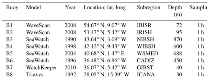
The study domain includes an array of buoys operated by Puertos del Estado and the Irish Marine Institute (Fig. 1a), providing quality-controlled hourly-averaged observations of SST, sea surface salinity (SSS) and currents. To ensure the continuity of the data record, occasional gaps detected in time series (not larger than 6 h) were linearly interpolated. Basic features of each in situ instrument are described in Ta-ble 2.
4.2.2 Satellite-derived observations
The European Ocean Sea Surface Temperature L3 Ob-servations is a CMEMS operational product which pro-vides a daily fusion of SST measurements from mul-tiple satellite sensors over a 0.02◦ resolution grid. The L3 multi-sensor (super-collated) product is built from bias-corrected L3 mono-sensor (collated) products. If the na-tive collated resolution is N and N <0.02◦ the change (degradation) of resolution is done by averaging the best quality data. If N >0.02◦ the collated data are associ-ated to the nearest neighbour without interpolation nor artificial increase in the resolution. A synthesis of the bias-corrected L3 mono-sensor (collated) files remapped at resolution R is done through a selection of data based on the following hierarchy: AVHRR_METOP_B, SE-VIRI, VIIRS_NPP, AVHRRL-19, AVHRRL-18, MODIS_A, MODIS_T, AMSR2. This hierarchy can be changed in time depending on the health of each sensor. Further details can be found in the Product User Manual (PUM), freely avail-able on the CMEMS website (http://cmems-resources.cls.fr/ documents/PUM/CMEMS-SST-PUM-010-009.pdf, last ac-cess: 1 July 2019)
4.2.3 HFR-derived observations
Table 2.Description of the network of directional buoys used in this work. Year label stands for year of deployment. Subregions are defined in Fig. 1a.
Buoy Model Year Location: lat, long Subregion Depth Sampling (m)
B1 WaveScan 2008 54.67◦N, 9.07◦W IBISR 72 1 h
B2 WaveScan 2008 53.47◦N, 5.42◦W IRISH 95 1 h
B3 SeaWatch 1990 43.64◦N, 3.09◦W NIBSH 870 1 h
B4 SeaWatch 1998 42.12◦N, 9.43◦W WIBSH 600 1 h
B5 SeaWatch 2004 40.68◦N, 1.47◦E WSMED 688 1 h
B6 SeaWatch 1996 36.48◦N, 6.96◦W CADIZ 450 1 h
B7 WatchKeeper 2010 36.07◦N, 5.42◦W GIBST 40 1 h
B8 Triaxys 1992 28.05◦N, 15.39◦W ICANA 30 1 h
averaging radius set to 3 km, in order to estimate hourly to-tal current vectors on a Cartesian regular grid of 1 km×1 km horizontal resolution.
A source of error to be considered in the computation of the total vectors is the so-called geometrical dilution of pre-cision (GDOP). The GDOP is defined as a dimensionless co-efficient of uncertainty that characterizes how radar system geometry may impact on the measurement accuracy and po-sition determination errors, owing to the angle at which ra-dial vectors intersect. Maps of east and north GDOP for this HFR system (not shown) follow a pattern where their values increase with the distance from the radar sites and along the baselines (lines connecting two HFR sites), as the combin-ing radial vectors are increascombin-ingly parallel and the orthogo-nal component tends to zero. Further details can be obtained from Lorente et al. (2018).
The accuracy of HFR measurements, which are affected by intrinsic uncertainties (radio frequency interferences, en-vironmental noise, etc.) have been previously assessed by comparing against in situ observations provided by a point-wise current meter (Lorente et al., 2014), yielding correla-tions above 0.7 and RMSD below 13 cm s−1. Such results revealed that this HFR network has been operating within tolerance ranges, properly monitoring the surface circulation in near-real time of this geostrategic region.
Recent work relying on this HFR system has successfully investigated the water exchange between Algeciras Bay and the Strait of Gibraltar (Chioua et al., 2017), the impact of the atmospheric pressure fluctuations on the mesoscale water dy-namics of the Strait of Gibraltar and the Alboran Sea (Dastis et al., 2018), the dominant modes of spatio-temporal vari-ability in the surface circulation (Soto-Navarro et al., 2016), or the characterization of the Atlantic surface inflow into the Mediterranean Sea (Lorente et al., 2018).
In the present work, quality-controlled hourly HFR cur-rent measurements collected during the entire 2017 were used as benchmark to elucidate the skill of a number of OOFSs. The data availability was significantly high: almost 100 % in the selected transect (solid black longitudinal line shown in Fig. 1c), decreasing in the easternmost sectors. The
transect used to examine the AJ surface inflow was readily chosen as the associated total GDOP, reported in Lorente et al. (2018); was reduced (below 1.3); and the spatial and temporal data availability were optimal during 2017. From an oceanographic perspective, the election of such a transect was also convenient to better characterize both the intensity and direction of the AJ, since its midpoint covers the area where the highest peak of current speed is usually detected and also where the inflow orientation is not influenced yet by the water exchange between Algeciras Bay and the Strait of Gibraltar.
5 Comparison between CMEMS model solutions in IBI waters
5.1 Temperature
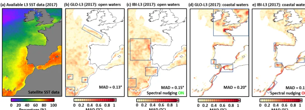
The CMEMS L3 satellite-derived daily data were used to val-idate the SST fields predicted by both GLOBAL and IBI sys-tems. The map of annual availability of this remote-sensing product for 2017 (Fig. 2a) reveals that the highest percent-ages of available observations (above 80 %) were found in the south of Canary Islands, the Gulf of Cádiz, and in the Western Mediterranean Sea. Equally, there was also a signif-icant data provision in the west coast of the Iberian Peninsula and Morocco, although it decreased to 70 % in nearshore ar-eas over the shelf such as the Iberian and African upwelling or the Strait of Gibraltar. By contrast, the lowest data avail-ability (below 40 %) was detected in the northernmost lati-tudes, including the Irish and North seas.
Figure 2. (a)Availability of satellite-derived L3 SST daily data for 2017;(b, c)annual mean absolute difference (MAD) of SST for 2017 in open water where the spectral nudging is applied: GLOBAL versus satellite and IBI versus satellite;(d, e)Analogous to(b, c)but in coastal waters where no spectral nudging is applied. Zones of worse model performance (i.e. higher MAD) are delimited with blue rectangles. Spatially averaged MAD values are provided in the lower-right corner.
(MAD=0.15◦), thereby allowing the regional and global model states to be reconciled with each other. IBI even outperformed GLOBAL locally in specific zones (delimited with blue rectangles in Fig. 2b) such as the western Ca-nary Islands, the periphery of Madeira Island, or a portion of the African coastal upwelling system. Furthermore, a narrow belt of SST anomalies could be observed along the continen-tal shelf break in the case of GLOBAL (Fig. 2b). Since IBI presents a higher grid resolution, it could partially resolve the internal waves breaking, which leads to turbulence and energy for increased vertical mixing with cooler waters be-neath the pycnocline, ultimately contributing to the reduced SST differences observed in IBI estimations over the conti-nental shelf break (Fig. 2c). By contrast, GLOBAL appeared to outperform IBI in the Gulf of Cádiz, the NW Iberian open water and the region between Canary and Madeira islands (Fig. 2c).
Maps of annual MAD in coastal areas (Fig. 2d and e), where no spectral nudging was imposed and the IBI sys-tem ran freely, exhibited some similarities such as the pro-nounced SST differences encountered in the Iberian and African coastal upwelling systems (ICUS and ACUS, re-spectively). According to the skill metrics, spatially aver-aged over the entire coastal waters domain, IBI performance was, on average, more accurate than GLOBAL (0.17◦ ver-sus 0.20◦) thanks to several factors (i.e. the more refined mesh and the tidal solution included in IBI). GLOBAL out-puts exhibited relevant SST differences over the continental shelf, especially in energetic tidally dominated areas such as the English Channel, the Irish Sea, and southern part of the North Sea (Fig. 2d). In these regions, monthly maps of SST bias (not shown) revealed the alternation between winter cold anomalies and summer warm anomalies, in accordance with
earlier results of Graham et al. (2018). Tidally driven ver-tical mixing could account for a portion of the discrepan-cies encountered between the coarser detided GLOBAL and IBI model solutions, where the former seems to predict an over-stratification in shelf seas. IBI also appeared to slightly outperform GLOBAL in some delimited areas of the Por-tuguese coast, the Gulf of Cádiz, and the ACUS (Fig. 2d). Besides, the higher SST anomalies observed for GLOBAL in the Strait of Gibraltar and the western Alboran Sea were likely linked to the inadequate representation of the speed and direction of the Atlantic Jet inflow, something that will be addressed in the following sections. On the contrary, it is also true that GLOBAL was to a little extent more precise in some parts of Western Mediterranean Sea, the ICUS, and ACUS (Fig. 2e).
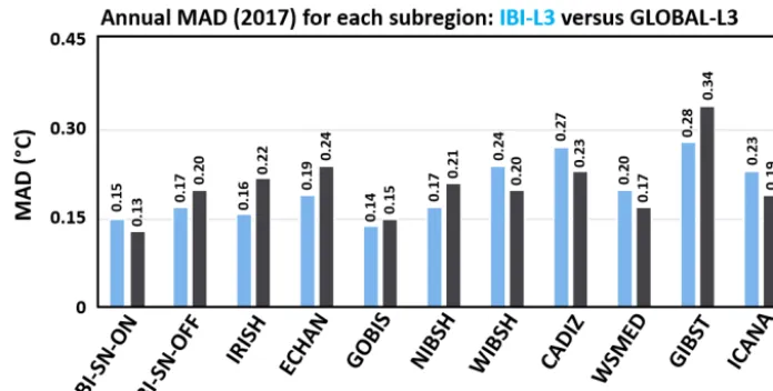
The MAD metrics for each subregion within the IBI re-gional domain (defined in Fig. 1a) are shown in Fig. 3. As above mentioned, IBI generally outperformed GLOBAL system in those subregions where no spectral nudging was applied (English Channel, Irish and North seas, North Iberian Shelf), with the exception of the Western Iberian Shelf (WIBSH). In addition, better metrics were obtained for IBI in the Gulf of Biscay (GOBIS), where the spectral nudg-ing was only applied in the westernmost off-shelf area. On the contrary, GLOBAL seemed to better replicate the SST field in the open sea thanks to the direct data assimilation. IBI metrics, albeit consistent, were slightly worse than those obtained for GLOBAL in this region.
Figure 3. Annual (2017) mean absolute difference (MAD) of SST, spatially averaged for each subregion (defined in Fig. 1a), between IBI (GLOBAL) and satellite L3 observations, represented by blue (black) columns. IBI-SN-ON (IBI-SN-OFF) represents the area where the spectral nudging technique was (was not) applied.
(not-assimilated) satellite-derived observations (CMEMS L3 gappy product) used as benchmark to comprehensively val-idate the models. Furthermore, satellite products are af-fected by intrinsic uncertainties. The quality information documents (QUIDs) focused on the accuracy assessment of OSTIA (McLaren et al., 2016) and L3 (Saux-Pickart et al., 2019) satellite products have reported a RMSD of 0.4◦ (0.2◦) between OSTIA (L3) and drifting buoys observations for 2012 (2018). More specifically, in the case of OSTIA estimations, the RMSD is 0.40◦globally with regional val-ues ranging from 0.28◦ in the South Pacific to higher val-ues in the North Atlantic (0.47◦) or in the Mediterranean Sea (0.89◦). By contrast, the L3 SST product shows reason-ably good difference statistics against drifting buoy measure-ments. This bias in satellite estimations should be taken into account when interpreting the results of the model valida-tions.
On the other hand, the highest SST discrepancies for both models were generally located in very coastal areas (African and Iberian upwelling systems, Strait of Gibraltar, etc.) and over the continental shelf (the Irish Sea and the English Channel) where satellite remote sensing could be compli-cated by weather patterns and dissolved organic compounds of terrestrial origin that may attenuate signals and yield unre-liable results (Thakur et al., 2018). As a consequence, many processed remote sensing products apply a land mask that excludes mixed pixels in nearshore areas, use temporal aver-aging to account for missing observations, or even impose an optimal interpolation process to transform the original satel-lite tracks into a regular grid (i.e. OSTIA product). In this context, the availability of the SST L3 data (Fig. 2a) was lower on the shelf near coastal areas featuring a complex bathymetry (likely due to poor satellite coverage, application
of a land mask, or cloud cover), justifying to some extent the predominance of SST anomalies near the shorelines.
For the sake of completeness, supplementary validation work in the entire 3-D water column with Argo floats is reg-ularly conducted to assess model vertical structure. For the period 2012–2016 and the entire IBI domain, the averaged RMSD for full profiles of temperature and salinity are 0.51◦ and 0.13 PSU, respectively (for further details, we refer the reader to the IBI QUID). Both models perform fairly well in open water, given the fact that GLOBAL assimilates these types of in situ observations and subsequently transfers the information to the nested IBI system thanks to the aforemen-tioned spectral nudging technique. Nevertheless, validation focused on smaller scales and high-frequency processes is still crucial to analyse in detail the performance of both mod-elled products in intricate coastal regions.
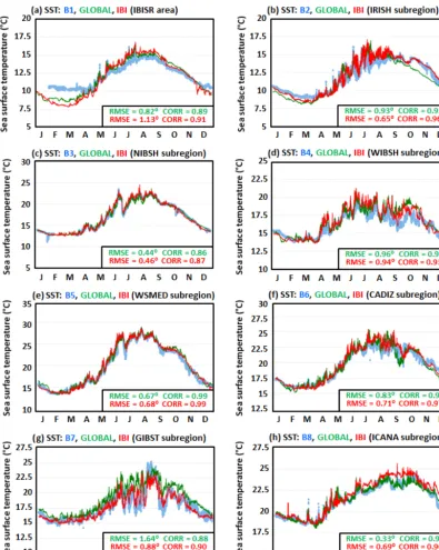
Hourly in situ observations from eight buoys, moored within specific subregions (Fig. 1a), were used as bench-mark to validate both GLOBAL and IBI outputs. The an-nual time series of SST exhibited a significantly high re-semblance, properly reproducing the expected annual-cycle shape (Fig. 4). According to the consistent skill metrics de-rived from the comparison against three deep-water buoys (B3, B4, and B5, in Table 2), both models had a rather simi-lar performance during 2017 with RMSD and correlation co-efficients in the ranges 0.44–0.96◦C and 0.86–0.99, respec-tively (Fig. 4c–e). While the similar behaviour observed off the shelf is partially attributable to the aforementioned spec-tral nudging technique, the model–observation comparison in near-shore areas revealed noticeable discrepancies.
Figure 4.Annual (2017) time series of hourly sea surface temperature (SST) at eight different locations within IBISR area. In situ observa-tions from moored buoys (blue dots), GLOBAL model predicobserva-tions (green line), and IBI model outputs (red line) are depicted. Skill metrics derived from model–observation comparison are gathered in black boxes.
for the Strait of Gibraltar are not in complete accordance with the statistics previously derived from the comparison against L3 satellite-derived data (Fig. 3j), likely due to the fact that remote-sensed SST estimation areas might be af-fected by higher intrinsic uncertainties (i.e. land contamina-tion and cloud cover). Although both comparisons against remote and in situ observations confirmed the model SST overestimation in GIBST, especially during summertime, the
to overestimate SST in this area during the entire year, as reflected by a RMSD of 1.64◦C.
On the other hand, GLOBAL seemed to behave slightly better at B1 location – IBISR area – (Fig. 4a) and sub-stantially more accurately at B8 buoy location – in the Ca-nary Islands, ICANA, – where a permanent SST overestima-tion from June to December was evidenced in IBI predic-tions (Fig. 4h), thereby yielding a RMSD twice higher than that obtained for GLOBAL estimations, in agreement with Figs. 2i–j and 3i. The lower performance of IBI in ICANA subregion was previously reported by Aznar et al. (2016) when inter-comparing IBI forecast and 1/12◦reanalysed so-lutions. At this point it is worth recalling that GLOBAL in-cludes a data assimilation scheme, whereas IBI takes realis-tic ocean conditions from weekly global analyses. This fact shows up the possible benefits of the observational data as-similation in these areas, at least in terms of surface variables. Furthermore, a fraction of observed model–buoy discrepan-cies in SST can be explained in terms of disparate depth scales. Whereas IBI and GLOBAL daily outputs are repre-sentative of the temperature in the upper 1 m of the water column, moored buoys provide temperature estimations at a deeper nominal depth (between 1 and 3.5 m, depending on the brand). Future validation exercises should include the in-terpolation of model outputs to both the exact buoy location and also to the specific depth level in order to more accurately assess the model skilfulness. It is worthwhile mentioning that a variety of previous work has focused on the comparison of in situ and remote-sensed SST data, reporting significant dif-ferences across different geographical regions (Thakur et al., 2018; Stobart et al., 2015; Smit et al., 2013). Such discrepan-cies could also be observed in this work as lower biases were generally derived from the pointwise comparisons, thereby highlighting the intrinsic uncertainties associated with satel-lite data in nearshore areas.
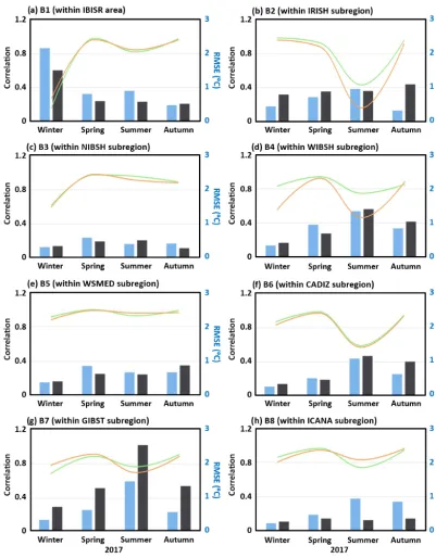
Complementarily, a quarterly analysis was performed to infer any potential degradation in model performances during a specific season of the year (Fig. 5). Overall, both GLOBAL and IBI predictions seemed to be more reliable in winter (ex-cept at B1 location, Fig. 5a) in terms of lower RMSD. They also emerged to be less realistic during summer, as denoted by abrupt decreases in quarterly correlation indexes (from 0.9 down to 0.5) at B2, B4, and B6 locations and the relevant rise of RMSD (up to 2.5◦C) at B7 location (GIBST subre-gion). This SST overestimation could be partially explained in terms of imprecise latent sensible heat fluxes and excess of evaporation, although additional efforts should be devoted to shed light on it. Once again, IBI performance appeared to be more accurate in coastal zones featuring a more com-plex bathymetry (at B2, B4, B6, and B7 locations), whereas GLOBAL fitted better to in situ observations in off-shelf re-gions such as at B1 and B8 locations. In the rest of the cases, both model solutions were rather similar. It is noteworthy that each pointwise buoy is not representative of the entire
subre-gion in which it is deployed, thus explaining to some extent the discrepancies arisen between Sect. 6.1 and 6.2.
5.2 Salinity
As pointed out in the introduction, the enhancement of river-ine forcing is still a priority in ocean modelling as the estuar-ine circulation is mainly driven by horizontal density gradi-ents which are ultimately modulated by freshwater inputs. In this context, previous work has investigated the poten-tial benefits of replacing old climatologies by data from hy-drological model predictions (O’Dea et al., 2017). Here we provide a specific example to illustrate the discrepancies be-tween GLOBAL and IBI performances in the Galician coast (NW Spain), as a consequence of the different horizontal res-olution and distinct runoff forcing implemented in the op-erational chain. While both model performances are rather similar in open water (according to the results derived from the validation against 3-D Argo-float profiles and exposed in the QUID), higher discrepancies are expected to arise in coastal and shelf areas as they are governed by small-scale processes such as land–sea breezes, runoff (and the resulting stratification and buoyancy-driven circulation), and transport materials (nutrients, sediments, pollutants, etc.).
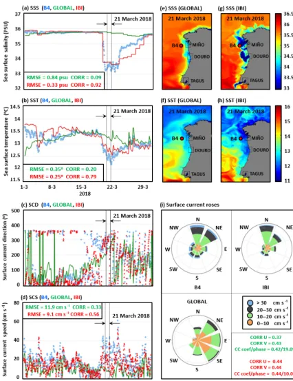
As shown in Fig. 6a, hourly in situ SSS data collected by B4 buoy during March 2018 experienced an abrupt decrease from a standard value around 36 PSU down to almost 33 PSU in just a few hours during 20 March, likely due to a noticeable filament of freshwater discharged by Miño River. IBI outputs at the closest grid point appeared to properly capture both the sharp drop in SSS values and the persistent low salinity val-ues for the next 4 d period. By the end of the month, the mod-elled salinity field seemed to steadily recover to usual levels in the range of 35.5–35.8 PSU, whereas in situ observations revealed a steeper rise to 34.8 PSU by 23 March. Neverthe-less, the skill metrics confirmed the rather accurate IBI per-formance, with a correlation coefficient of 0.92 and a RMSD of 0.33 PSU. By contrast, although GLOBAL outputs could replicate the mean SSS, it did not reproduce satisfactorily the freshwater episode and barely showed any temporal variabil-ity, as reflected by a negligible correlation coefficient (0.09) and a higher RMSD (0.84 PSU).
Figure 5.Annual evolution (2017) of seasonal skill metrics derived from the comparison of GLOBAL and IBI models against in situ SST hourly observations provided by eight buoys. RMSD and correlation coefficient represented by coloured bars and lines, respectively.
and map of HFR-derived surface currents for May 2018 (not shown) did not exhibit the well-documented conditions as-sociated with NW Iberian upwelling episodes, such as the predominant northerly winds and the subsequent offshore de-flection of the surface flux, respectively.
The buoyancy input introduced by large freshwaters fluxes (particularly during the spring freshet), together with
vailing surface flow as modelled currents were mainly ad-vected to the south-southwest (180–270◦). Equally, IBI ap-peared to correctly replicate the acceleration of the upper-layer stream from 10 to 45 cm s−1 due to impulsive-type freshwater river outflow already observed in situ estimations of sea surface currents (Fig. 6d). Notwithstanding, GLOBAL current intensity remained moderate (below 20 cm s−1) dur-ing most of March, includdur-ing the selected episode, as re-flected by the poorer skill metrics obtained. The current speed underestimation observed in this tidal environment is mainly attributable to the fact that GLOBAL system provides a detided solution, so barotropic tidal velocities do not con-tribute to the final prescribed total velocity.
Daily-averaged maps of modelled SSS and SST were com-puted for 21 March (Fig. 6e–h) to infer the differences be-tween GLOBAL and IBI. As it can be seen, the former showed a relatively smoothed and spatially homogeneous de-crease in the salinity and temperature fields along the entire coastline (Fig. 6e and f), while the latter exhibited more intri-cate patterns with many filaments together with a significant drop in SSS and SST (Fig. 6g and h) in the periphery of the three main local river mouths (from north to south: Miño, Douro, and Tagus) as a result of freshwater plumes outflow-ing over saltier Atlantic waters. In the three cases, the SST field could effectively act as a tracer for the salinity stratifi-cation.
There is a significant resemblance between the monthly current roses derived from in situ observations and IBI pre-dictions in terms of speed and mean direction (Fig. 6i), showing the predominance of the so-called Iberian Poleward Current, flowing northwards and circuiting the western and northern Iberian margins under prevailing southerly winds (Torres and Barton, 2006). GLOBAL current outputs differed from observations, exhibiting an overall tendency for east-ward directions. The skill metrics derived from time series comparison at B4 buoy location confirmed that the regional OOFS outperformed the global one during March 2018, hence postulating the benefits of improved horizontal reso-lution to better resolve the plume dynamics and its exten-sion off shelf. In addition, the increased horizontal resolution of IBI allows us to better resolve individual frontal fluctua-tions and horizontal salinity gradients by preserving the sig-nal of river plume closer to the coast and with a more com-plex structure. The impact of model resolution in both the horizontal extent of the plume and the strength and position of the freshwater front has been subject of previous studies (Bricheno et al., 2014). Since both models present 50 depth levels and similar vertical discretization, the horizontal reso-lution and the riverine forcing are assumed to play a primary role when attempting to explain the differences encountered in model performance for this specific test case.
6 Circulation in the Strait of Gibraltar: multi-model comparison from global to coastal scales
Proved the relevance of the intensity and orientation of the AJ in determining the surface circulation of the Alboran Sea, the ability of each OOFS to portray the upper layer circulation in the GIBST area has been evaluated. The annually averaged surface pattern provided by the HFR network revealed north-eastward speeds around 100 cm s−1in the narrowest section of the strait (Fig. 7a). SAMPA coastal model seemed to cap-ture well the time-averaged intensity and orientation of the Atlantic inflow (Fig. 7b), whereas IBI regional model clearly overestimated the mean surface circulation speed (Fig. 7c). Finally, the coarser OOFS (GLOBAL) barely captured the most basic features on the incoming flow and its subsequent propagation towards the northeast (Fig. 7d).
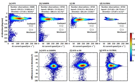
As this qualitative model intercomparison on a yearly ba-sis was insufficient to infer the skilfulness of each system, a quantitative validation at the midpoint of the selected transect (white square in Fig. 1c) was assessed. The scatter plot of HFR-derived hourly current speed versus direction (taking as reference the north and positive angles clockwise) revealed interesting details (Fig. 8a): firstly, the AJ flowed predom-inantly eastwards, forming an angle of 78◦ with respect to the north. The current velocity, on average, was 100 cm s−1 and reached peaks of 250 cm s−1. Speeds below 50 cm s−1 were registered along the entire range of directions. West-wards currents, albeit in the minority, were also observed and tended to predominantly form an angle of 270◦.
The scatter plot of SAMPA estimations presented a signif-icant resemblance in terms of prevailing current velocity and direction (Fig. 8b). Although the time-averaged speed and angle were slightly smaller (90 cm s−1) and greater (88◦), spectively, the main features of the AJ were qualitatively re-produced: maximum velocities (up to 250 cm s−1) were as-sociated with an eastward flow and an AJ orientation in the range of 50–80◦. Besides, surface flow reversals to the west were properly captured.
By contrast, noticeable differences emerged in the scat-ter plot of regional IBI estimations (Fig. 8c): surface current velocities below 30 cm s−1 were barely replicated and the AJ inversion was only observed very occasionally. Despite the fact that IBI appeared to properly portray the mean char-acteristics of the eastwards flow, the model tended to favour flow directions comprised between 60 and 180◦and to over-estimate the current velocity, with averaged and maximum speeds around 117 and 280 cm s−1, respectively.
In the case of the scatter plot derived from GLOBAL es-timations, even more substantial discrepancies were detected as the variability in both the AJ direction and speed were clearly limited to the range 65–80◦ and 50–200 cm s−1, re-spectively (Fig. 8d). No flow reversals were detected and peak velocities of the eastward flow were underestimated.
Figure 7.Annual mean circulation pattern in GIBST for 2017, derived from hourly estimations provided by(a)HFR,(b)SAMPA coastal model,(c)IBI regional model, and(d)GLOBAL model. For the sake of clarity, only one vector for every two was plotted in the HFR map.
Figure 8. (a–d)Annual (2017) scatter plot of hourly AJ current speed versus direction (angle measured clockwise from the north); estimations provided by(a)HFR,(b)SAMPA,(c)IBI, and(d)GLOBAL. Mean and standard deviation values of both AJ speed and direction are gathered in black boxes;(e–g)annual scatter plot of differences (observation minus model) in AJ speed and direction between(e)HFR and SAMPA,
(f)HFR and IBI, and(g)HFR and GLOBAL.
SAMPA, discrepancies were clustered around zero for both parameters, with an asymptotic distribution along the main axes (Fig. 8e). On the contrary, a negative bias to negative differences was observed for both IBI (Fig. 8f) and GLOBAL (Fig. 8g), especially for the latter. In other words, the regional and global OOFSs overestimated both the current speed and the angle of the AJ, reflecting a tendency for more southeast-erly directions (clockwise rotated with respect to the north). Overall, a steady improvement in the AJ characterization is evidenced in model performance when zooming from global to coastal configurations, highlighting the benefits of the
the entire Mediterranean basin, which is only partially in-cluded in IBI and GLOBAL systems, plays a major role not only in the regulation of the seasonal cycle of the AJ but also in the occasional inflow inversions, in accordance with previ-ous work (Macias et al., 2016). Since the atmospheric pres-sure forcing is missing in the GLOBAL sea level outputs, this system only considers the barotropic response to wind forc-ing. In the case of IBI system, both atmospheric forcings are taken into account but the inverted barometer approximation is solely imposed over the Western Mediterranean Sea (not over the entire basin). Therefore, only a portion of the subti-dal variability in the flow through the Strait of Gibraltar can be adequately explained (García-Lafuente et al., 2002b).
Additional statistical indicators were computed: two his-tograms illustrated the number of hourly zonal (U) and meridional (V) velocity data per class interval (Fig. 9a and b). HFR-derived zonal velocity estimations exhibited a Gaussian-like shape clustered around 84 cm s−1and slightly shifted to lower values in the case of SAMPA coastal model (79 cm s−1). Both datasets show similar positive skew and variability, with the standard deviation around 56–57 cm s−1 for 2017 (Fig. 9a). IBI and GLOBAL presented narrowed histograms, with distributions positively shifted and con-strained to zonal velocities above 0 and 40 cm s−1, respec-tively. In the case of meridional currents, each distribution exhibits a nearly symmetrical Gaussian-like shape but shifted towards different values (Fig. 9b). Whilst SAMPA and IBI exhibited a similar distribution (and moderately similar to that revealed for HFR estimations), GLOBAL histogram emerged again dramatically shortened and restricted only to positive values, revealing a recurrent predominance of the AJ to flow northeastwards.
Based on the QQ plot for the zonal velocity compo-nent (Fig. 9c), it can be concluded that SAMPA estimations were consistent despite the slight overestimation observed for the highest velocities (95th–100th percentiles). The gen-eral IBI overestimation along the entire range of percentiles was also clearly evidenced. In accordance with its histogram, GLOBAL system overestimated (underestimated) zonal cur-rents below (above) the 90th percentile. A similar behaviour was also observed for GLOBAL meridional velocities, this time around for the 20th percentile (Fig. 9d). On the con-trary, both SAMPA and IBI appeared to generally underes-timate the meridional surface current speed, even more for higher percentiles.
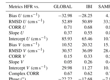
Class-2 skill metrics, gathered in Table 3, were also com-puted in order to provide a quantitative perspective of model performance at the midpoint of the selected transect (white square in Fig. 1c). SAMPA clearly outperformed both sys-tems, as reflected by lower RMSD values for both veloc-ity components together with a complex correlation coef-ficient (CCC) and phase (CCP) of 0.79 and −8◦, respec-tively, which means that SAMPA predictions were highly correlated with HFR current observations although slightly clockwise rotated (i.e. more southeastwards). The agreement
Table 3.Skill metrics derived from the 1-year (2017) validation of sea surface currents estimated by three operational forecasting sys-tems against HFR-derived observations at the midpoint of the se-lected transect in the Strait of Gibraltar (Fig. 1c).
Metrics HFR vs. GLOBAL IBI SAMPA
BiasU(cm s−1) −32.98 −28.25 4.17
RMSDU(cm s−1) 52.89 50.89 33.58
CORRU 0.71 0.68 0.83
SlopeU 0.37 0.55 0.82
InterceptU(cm s−1) 85.93 65.46 10.77
BiasV (cm s−1) 10.52 20.32 15.19
RMSDV (cm s−1) 30.57 36.09 28.48
CORRV 0.15 0.33 0.56
SlopeV 0.05 0.26 0.41
InterceptV (cm s−1) 29.98 11.27 10.17
Complex CORR 0.67 0.62 0.79
Phase (◦) −22.72 −12.68 −7.86
between HFR hourly data and IBI and GLOBAL estima-tions, albeit significant (CCC above 0.6), was lower as the related phase values decreased substantially (especially for GLOBAL: CCP below−20◦), indicating a more zonal sur-face flow.
The three systems predicted more precisely the zonal ve-locity component than the meridional one, with scalar corlations emerging in the ranges 0.68–0.83 and 0.15–0.56, re-spectively. Notwithstanding, RMSD values were more mod-erate for the latter (below 37 cm s−1) than for the former (be-low 53 cm s−1). This could be attributed to the extremely in-tense and predominant west–east zonal exchange of Atlantic-Mediterranean waters through GIBST, with the meridional flow playing a residual role.
The statistical results derived from SAMPA–HFR compar-ison, gathered in Table 3, are in line with those earlier ob-tained in a 20-month validation performed by Soto-Navarro et al. (2016), which reported correlations of 0.70 and 0.27 for the zonal and meridional velocities, respectively. The ob-served model–radar discrepancies might be attributed to the fact that the uppermostzlevel of SAMPA model is 2.5 m, while HFR observations are representative of the first 0.5 m of the water column and thus more sensitive to wind forcing. This might explain some model drawbacks detected in rela-tion to the reduced energy content in surface current speeds, as reflected by the positive bias between HFR estimations and SAMPA outputs (Table 3).
Figure 9.Annual (2017) histogram of hourly(a)zonal current velocities and(b)meridional current velocities, as provided by HFR, SAMPA, IBI, and GLOBAL. Mean and standard deviation values are gathered in black boxes. Quantile–quantile plots of hourly(c)zonal current ve-locities and(d)meridional current velocities, as derived from the observation–model comparison. The 10 %–99 % quantiles were established (red filled dots).
level pressure (SLP: Fig. 10a–d) and zonal wind at 10 m height (U−10: Fig. 10e–h). A significant latitudinal gradi-ent of SLP was observed in three episodes (February, March, and December), with high pressures over the Gulf of Bis-cay and isobars closely spaced in GIBST, giving rise to very strong easterlies (above 10 m s−1), channelled through the strait (Fig. 10e, f, and h). In August, the typical summer
weather type was observed with Azores High pressures gov-erning the Atlantic area and moderate but persistent easterly winds blowing through the entire Western Mediterranean Sea (Fig. 10c and g).
Figure 10.Two-day averaged synoptic maps of(a–d)sea level pressure (SLP) and(e–h)zonal wind at 10 m height (U-10), provided by ECMWF, corresponding to each of the four Atlantic inflow reversal events analysed during 2017.(i–l)Monthly time series of SLP, spatially averaged over the Western Mediterranean Sea (WSMED) subregion, marked with a big red box in the maps of the first row;(m–p)monthly time series of U-10, spatially averaged over the Strait of Gibraltar (GIBST) subregion, marked with a small red box in the maps of the second row;(q–t)monthly Hovmöller diagrams of HFR-derived zonal current velocity at the selected transect. Red (blue) colour represent eastward (westward) flow;(u–x)monthly time series of hourly sea surface height (SSH) provided by Tarifa tide gauge, represented by a blue dot in Fig. 1. Two-day episodes of permanent flow reversal are marked with black boxes in(i–x).
along the selected months (Fig. 10i–p). Very high SLP val-ues and extremely high (negative)U−10 (i.e. intense east-erlies) led to a complete inversion of the surface flow from the prevailing eastward direction to a westward outflow into the Atlantic Ocean, as reflected in the Hovmöller diagrams computed for the HFR-derived zonal currents (Fig. 10q– t). In February, a brief 24 h inversion (related to less
between weaker eastward and westward currents were evi-denced, mainly associated with changes in the prevalent wind regime (Fig. 10s and t). Under persistent easterlies, a weaker coastal counter current was detected flowing westwards and bordering the Spanish shoreline (Fig. 10s). Such coastal flow inversion has been previously reported and subject to further analysis by Reyes (2015). Particularly, the flow reversal de-tected in August was not triggered by high SLP (Fig. 10k) but induced by moderate and persistent easterlies (5 m s−1, Fig. 10o).
Short-lived reversals of the surface inflow have been pre-viously reported to occur almost every tidal cycle in Ca-marinal Sill (western end of GIBST: Fig. 1b) mainly due to the contribution of the semidiurnal tidal component M2 (Reyes, 2015; Sannino et al., 2004; García-Lafuente et al., 1990; La Violette and Lacombe, 1988). Since the mean in-flow of Atlantic water is modulated by barotropic tidal cur-rents, hourly-averaged sea surface height (SSH) observations provided by Tarifa tide gauge (Fig. 1c) were used to elucidate if the four 2 d inflow reversal events in the eastern end of the strait could have been mostly influenced by spring–neap tidal cycle fluctuations (Fig. 10u–x). Although the fortnightly variability was clearly observable in a monthly time series of SSH, no cause–effect relationship could be visually inferred from the inspection of zonal velocities at the selected tran-sect (Fig. 10q–t). Apparently, evidence of preference for a specific tidal cycle was not observed as the four flow reversal episodes took place under strong easterlies but during dif-ferent tidal conditions, ranging from neap tides (Fig. 10u) to spring tides (Fig. 10v and x). As shown in Lorente et al. (2018), tides seemed to play a secondary role by partially speeding up or slowing down the westward currents, depend-ing on the phase of the tide. These results are in accordance with previous modelling studies (Sannino et al., 2004) where the contribution of the semidiurnal tidal component to the transport was proved to be relevant over the Camarinal Sill, (incrementing the mean transport by about 30 % for both the inflow and the outflow), whereas it was almost negligible at the eastern end of the strait.
The observed 2 d averaged HFR-derived circulation pat-terns associated with the four events here studied are de-picted in Fig. 11a, e, i, and m. Some common peculiarities were exposed, such as the overall westward outflow through the narrowest section of GIBST or the subtle anticyclonic inflow into the Algeciras Bay. Three study cases revealed a predominant circulation towards the west together with a marked acceleration of the flow in the periphery of Algeci-ras Bay, reaching speeds above 70 cm s−1(Fig. 11a, e, and i). The fourth case (December 2017) was substantially less en-ergetic and exhibited a rather counter-clockwise recirculation in the entrance to GIBST (Fig. 11m). On the other hand, two episodes illustrated how the circulation in the easternmost region of the study domain followed a clockwise rotation (Fig. 11e and m).
From a qualitative perspective, SAMPA was able to repro-duce fairly well at least two of the four inversion episodes in terms of overall circulation pattern in GIBST and adjacent waters (Fig. 11f, j, and n). In the event of March, SAMPA replicated the intense eastern anticyclonic gyre, with veloci-ties up to 80 cm s−1, along with the inflow into the Algeciras Bay. However, the model could only partially resolve the AJ inversion, exhibiting a counter-clockwise recirculation with the outflow restricted to the northwestern Spanish shoreline (Fig. 11f). In the episode corresponding to 4–5 December (Fig. 11n), the upper-layer dynamic was rather similar to the one previously described for March, albeit less vigorous. The visual resemblance with the HFR map (Fig. 11m) was gener-ally high, according to common features observed: the east-ern anticyclonic gyre, the central belt of currents circulating towards the northwest and eventually the cyclonic recircu-lation structure in the entrance to GIBST. On the contrary, in the event that occurred between 14–15 August (Fig. 11j), a moderate observation–model resemblance was deduced in the northeastern sector of the domain: SAMPA was able to resolve the observed southwestward stream, the inflow into the Algeciras Bay, and the weak intrusion of Mediterranean waters into GIBST bordering the northern shoreline but, by contrast, it was ultimately impelled to join the general AJ in-flow governing the strait and propagating towards the east. Finally, although SAMPA predicted the occurrence of AJ reversal by 20—21 February (Fig. 11b), the simulated cir-culation structure partially differed from that observed with HFR estimations (Fig. 11a). Whereas the former prognosti-cated a meander-like circulation, a predominant cross-shore stream within the channel and a flow inversion uniquely cir-cumscribed to the entrance of GIBST; the latter provided an overall westward outflow from the Mediterranean Sea into the Atlantic Ocean.