https://doi.org/10.5194/esd-9-895-2018
© Author(s) 2018. This work is distributed under the Creative Commons Attribution 4.0 License.
Modelling feedbacks between human and
natural processes in the land system
Derek T. Robinson1, Alan Di Vittorio2, Peter Alexander3,4, Almut Arneth5, C. Michael Barton6, Daniel G. Brown7, Albert Kettner8, Carsten Lemmen9, Brian C. O’Neill10, Marco Janssen11, Thomas A. M. Pugh12,13, Sam S. Rabin5, Mark Rounsevell3,5, James P. Syvitski14, Isaac Ullah15, and
Peter H. Verburg16
1Department of Geography and Environmental Management,
University of Waterloo, Waterloo, Ontario, Canada 2Climate and Environmental Sciences Department, Lawrence
Berkley National Laboratory, Berkeley, California, USA
3School of Geosciences, University of Edinburgh, Drummond Street, Edinburgh, EH8 9XP, UK 4Land Economy and Environment Research, SRUC, West Mains Road, Edinburgh, EH9 3JG, UK
5Karlsruhe Institute of Technology, Institute of Meteorology and Climate Research –
Atmospheric Environmental Research (IMK-IFU), Garmisch-Partenkirchen, Germany 6School of Human Evolution & Social Change and Center for Social
Dynamics and Complexity, Arizona State University, Tempe, Arizona, USA
7School of Environmental and Forest Sciences, University of Washington, Seattle, Washington, USA 8Dartmouth Flood Observatory,12Community Surface Dynamics Modeling System, Institute
of Arctic and Alpine Research, University of Colorado, Boulder, Colorado, USA 9Institute of Coastal Research, Helmholtz-Zentrum Geesthacht, Geesthacht, Germany
10National Center for Atmospheric Research, Boulder, Colorado, USA 11School of Sustainability, Arizona State University, Tempe, Arizona, USA
12School of Geography, Earth and Environmental Sciences, University of Birmingham, Birmingham, UK 13Birmingham Institute of Forest Research, University of Birmingham, Birmingham, UK 14Community Surface Dynamics Modeling System, University of Colorado, Boulder, Colorado, USA
15Department of Anthropology, San Diego State University, San Diego, California, USA 16Environmental Geography Group, Institute for Environmental Studies,
VU University Amsterdam, Amsterdam, the Netherlands
Correspondence:Derek T. Robinson ([email protected])
Received: 28 June 2017 – Discussion started: 12 July 2017 Revised: 10 April 2018 – Accepted: 14 May 2018 – Published: 26 June 2018
896 D. T. Robinson et al.: Modelling feedbacks between human and natural processes in the land system
development and experience associated with the four models of coupled human–natural systems, the following eight lessons were identified that if taken into account by future coupled human–natural-systems model devel-opments may increase their success: (1) leverage the power of sensitivity analysis with models, (2) remember modelling is an iterative process, (3) create a common language, (4) make code open-access, (5) ensure consis-tency, (6) reconcile spatio-temporal mismatch, (7) construct homogeneous units, and (8) incorporating feedback increases non-linearity and variability. Following a discussion of feedbacks, a way forward to expedite model coupling and increase the longevity and interoperability of models is given, which suggests the use of a wrap-per container software, a standardized applications programming interface (API), the incorporation of standard names, the mitigation of sunk costs by creating interfaces to multiple coupling frameworks, and the adoption of reproducible workflow environments to wire the pieces together.
1 Introduction
Models designed to improve our understanding of human– environment interactions simulate interdependent processes that link human activities and natural processes but usually with a focus on the human or natural system. When simulat-ing the land system, such models tend to incorporate either detailed decision-making algorithms with simplified ecosys-tem responses (e.g. land-use models) or simple mechanisms to drive land-cover patterns that affect detailed environmen-tal processes (e.g. ecosystem models). These one-sided ap-proaches are prone to generating biased results, which can be improved by capturing the feedbacks between human and natural processes (Verburg, 2006; Evans et al., 2013; Roun-sevell et al., 2014). Hence, improving our understanding of the interdependent dynamics of natural systems and land change through modelling remains a key opportunity and im-portant challenge for Earth-system research (NRC, 2013).
Land use describes how humans use the land and the ac-tivities that take place at a location (e.g. agricultural or forest production), whereas land-cover change describes the transi-tion of the physical surface cover (e.g. crop or forest cover) at a location. These distinct concepts are inextricably linked, and modellers sometimes conflate them or, when represented separately, fail to link them. Because of the tradition of divi-sion between human and natural sciences (Liu et al., 2007), land-change science and social science have focused on how socio-economic drivers interact with environmental variabil-ity to affect new quantities and patterns of land use (Turner II et al., 2007) while natural science has focused on modelling natural-system responses to prescribed land-cover changes (e.g. Lawrence et al., 2012).
An important limitation of most natural-system models1 is that the impacts of human action are represented through changes in land cover that rarely involve mechanistic de-scriptions of the human decision processes driving them. These models are typically applied at coarse resolutions and ignore the influence of critical land management activities on natural processes and micro-to-regional climate associ-ated with fine-resolution factors such as landscape configura-tion (e.g. Running and Hunt, 1993; Smith et al., 2001, 2014; Robinson et al., 2009), fragmentation and edge effects (e.g. Parton et al., 1987; Lawrence et al., 2011), and horizontal energy transfers (e.g. Coops and Waring, 2001). The conse-quences of excluding these factors on the representation of natural processes can be significant because they aggregate to affect global processes.
Conversely, efforts to model and represent changes in how land is used by humans (i.e. land-use change mod-els, LUCMs) have been developed to understand how hu-man processes impact the environment but in ways that often oversimplify the representation of natural processes (Evans et al., 2013). While such models vary in their level of pro-cess detail, they usually include some representation of the economic and social interactions associated with alternative land-use types. Over the past 5–10 years, the representation of natural systems has been improved in LUCMs by system-atically increasing the complexity of natural processes repre-sented from inventory approaches to rule-based approaches
1Natural-system model is used as an overarching term for Earth
(e.g. Manson, 2005), statistical models (e.g. Deadman et al., 2004), dynamic linking to ecosystem models (e.g. Matthews, 2006; Yadav et al., 2008; Luus et al., 2013), or coupling of integrated assessment models and Earth-system models (e.g. Collins et al., 2015a). Even with the impetus to better under-stand human–environment interactions through model cou-pling, land-use science and the natural sciences have histor-ically been separate fields of scientific inquiry (Liu et al., 2007) that foster domain-specific methods and research ques-tions. Novel integrative modelling methods are being devel-oped to create technical frameworks for, and intersecting ap-plications between, these two communities (e.g. Theurich et al., 2016; Lemmen et al., 2018a; Peckham et al., 2013; Robinson et al., 2013a; Collins et al., 2015a; Barton et al., 2016; Donges et al., 2018) that offer insight and an initial benchmark for identifying methods for improvement.
The promise of greater integration between our represen-tations of human and natural processes lies partly in the spa-tially distributed representations of land use, land cover, veg-etation, climate, and hydrologic features. Models in land-change and natural sciences tend to contain a description of the land surface (often gridded) and, while the repre-sentations of these systems may differ in their level of de-tail, they are often complementary, thus facilitating a more complete representation and understanding of land surface change through integration. The coupling of land-change and natural-system models promises a new approach to charac-terizing and understanding humans as a driving force for Earth-system processes through the linked understanding of land use and land cover as an integrated land system.
The potential gains from greater coupling are threefold. First, the use of many of the Earth’s resources by humans al-ters the state and trajectory of the Earth system (Zalasiewicz et al., 2015; Waters et al., 2016; Bai et al., 2015). Therefore, representing and quantifying the impact of humans on the natural system can determine their magnitude relative to pro-cesses endogenous to the natural system as well as provide insight into how to mitigate those impacts through changes in human behaviour. Second, the natural system (e.g. cli-mate variability and change, extreme weather events, pro-cesses affecting soil fertility) also affects human propro-cesses. Therefore, interactions and feedbacks within the social and in socio-ecological systems must be better quantified (Ver-burg et al., 2016). Achieving substantive gains in our under-standing of coupled human–natural systems requires a crit-ical assessment of the different modelling approaches used to couple representations of human systems with natural sys-tems that range from local ecological and biophysical pro-cesses (e.g. erosion, hydrology, vegetation growth) through to global processes (e.g. climate). Third, coupled models will be most useful if we can use them to test possible interven-tions (e.g. policies or technologies) in the human or natural system and identify feedbacks that amplify or dampen sys-tem responses, thus garnering a better understanding about how human impacts on the environment can be mitigated and
how humans might anticipate and adapt to resulting changes in the natural system.
The coupled modelling approaches discussed here are used in other fields as well, for example in integrated as-sessment modelling (IAM; see Verburg et al., 2016), which combines human and natural systems and often explicitly incorporates feedbacks between the two systems. However, many IAMs use relatively simple representations of individ-ual systems in order to analyze the nature of interactions between them. In contrast, we focus on coupled modelling that combines specialized and more process-rich representa-tions of both and therefore may lead to different conclusions. Furthermore, new technology for model sharing, model cou-pling, and high-performance computing make it possible to connect specialized models, which was not possible when IAMs were first conceptualized 25 years ago. Because of the greater degree of openness enabled by these technologies and their modular nature, coupled models enable a greater degree of transparency in how we represent human–natural-system models. Whether their relative process richness enables a greater degree of model accuracy remains to be tested.
We present multiple approaches to coupling land-change and natural-system models and reflect on how their represen-tations of feedbacks add value to scientific inquiry into the dynamics of coupled human–natural systems. We highlight four example models that explicitly represent feedbacks be-tween land change and natural systems but vary in their scale of application and coupling architecture. We then present the lessons learned from the modelling research teams, discuss the challenges of representing feedbacks, and then outline a way forward to expedite model coupling initiatives and their subsequent scientific advances.
Approaches to model coupling
When two models communicate in a coordinated fashion, they form a coupled model, where the constituents are of-ten termed components (Dunlap et al., 2013). One of the first examples of coupled models was developed in the 1970s to describe the interaction of different physical processes represented by numerical models for weather prediction (e.g. Schneider and Dickinson, 1974). Model coupling has been expanded since then to encompass domain coupling, i.e. the coordinated interaction of models for different Earth-system domains or “spheres” (e.g. biosphere and atmo-sphere). Recent coupling frameworks implement coupling of functional units regardless of the process-versus-domain di-chotomy (e.g. MESSy cycle 2, Jöckel et al., 2005; Kerkweg and Jöckel, 2012).
communica-898 D. T. Robinson et al.: Modelling feedbacks between human and natural processes in the land system
Figure 1. Approaches to model coupling. (a) Loose model in-tegration via file/data exchange between model 1 (M1) and model 2 (M2);(b)models may manipulate parameters, variable val-ues, or the scheduling of processes in another model but they inter-act with independent data (i.e. model inputs and outputs);(c)the behaviour of models is the same as(b)except that they also affect each other by interacting with the same data (i.e. the output of one model may be used as the input for another);(d)a coupler coor-dinates run time and scheduling and may pass some information between models, models may also interact through manipulating data (model input and output files); (e)a coupler coordinates the run time and scheduling of the individual models and passes infor-mation between models that primarily use their own data;(f)the coupler coordinates all interactions between models and data.
tion. The simple characterization along a continuum from loose to tight neglects multidimensional nuances of differ-ent coupling configurations (Fig. 1), degree of coordination, and communication frequency (Fig. 2). However, the terms loose and tight coupling provide a shorthand about the ease and level of code integration, the required understanding of model components, and where the responsibility for code de-velopment resides.
In a strict implementation of loose coupling, communica-tion is mostly based on the exchange of data files (Fig. 1a) and coordination is the automated or manual arrangement of independently operating (and different) components and ex-ternally organized data exchange. No interaction of the devel-opers of the components is required, and coupling can extend across different expert communities and platforms. However, in many cases model modification is necessary to manipu-late the data generated by a model for use by another and to sequence that transaction. As we increase the frequency of communication between two models and the coordination of interaction (Fig. 2), we move towards a tight coupling. In a strict implementation of tight coupling – some call this the monolithic approach – all components and their coordina-tion is programmed within a single model; they share much of their programming code and access shared memory for communication.
Many existing instances of coupled models employ inter-mediate degrees of coupling. Existing technologies (i.e.
cou-Figure 2.Conceptual outline of the frequency of model commu-nication and coordination of interaction between models from no coupling to one-way and two-way feedback. Examples are not ex-haustive but illustrate common approaches used. M1: model 1; M2: model 2; T1: time step 1; Tn: time stepn. Initial conditions, where one model is merely used to set the initial conditions of another; pe-riodic perturbations, whereby one model updates data or variables used by another periodically and unilaterally; prescription, which is common to climate models that use a prescribed trajectory of land-cover data that do not endogenously change; periodic two-way feedback, whereby two different modelled processes may act at dif-ferent temporal resolutions and feedbacks occur upon alignment; and two-way feedback where the modelled processes are dependent on the results and behaviour of each other.
interaction between two or more models in terms of the pass-ing of data, manipulation of parameters, and schedulpass-ing of processes between models and in some cases directing mod-els to data or preprocessing data for use by a model. Typi-cally, couplers are designed for independent research projects using known and available software (e.g. R) and program-ming languages (e.g. Java, C++, Fortran). When a coupler has been designed for general use across multiple projects, the result is a coupling framework that enables the instan-tiation of multiple model coupling projects by others. Like existing modelling frameworks, a coupling framework can speed up the coupling process and facilitate the interaction, adoption, and comparison of different instantiated and cou-pled models.
Couplers or coupling frameworks (Fig. 1d–h) are typi-cally introduced when a modelling project becomes mul-tidisciplinary and requires collaborative modelling of sev-eral scientific disciplines, such that the coupled model is too complex to be comprehended by a single individual or re-search group (Voinov et al., 2010). For example, the Com-munity Surface Dynamics Modeling System (CSDMS; Peck-ham et al., 2013) promotes distributed expertise and inde-pendent models in the domain of Earth-surface dynamics. All components are required to implement basic model in-terfaces (BMIs) as communication ports with any other com-ponents in CSDMS (Syvitski et al., 2014). Similarly, to en-able interaction through a coupling framework (Fig. 1d), it has been suggested that all components implement the Earth System Modeling Framework (ESMF; Theurich et al., 2016), The Modular System for Shelves and Coasts (MOSSCO; Lemmen et al., 2018a) provides an example of this approach and combines the high-performance computing (HPC) capa-bility of ESMF with the distributed expertise of CSDMS to facilitate access to HPC for those working to couple models without expertise with HPC.
The degree of coupling is important as a technical design question, as depicted in Fig. 1, but also as an important onto-logical question affecting how well we can represent feed-backs within and among human and environment systems (Ellis, 2015; Liu et al., 2015; Dorninger et al., 2017). Taken together, the frequency of communication and degree of co-ordination affect the degree to which feedbacks can be repre-sented in coupled systems and, therefore, considered in our prediction of system behaviour or response to interventions (Fig. 2). For this reason, we describe four examples of cou-pled representations of human and natural systems, across a range of processes represented and scales of application, and how their coupling design affects the representation of feed-backs.
The four examples are situated at different points along the three dimensions of configuration, the frequency of commu-nication, and coordination. The first example uses a coupler in its architecture (similar to Fig. 1d and f) and achieves two-way coupling (Fig. 2) to investigate the effects of land man-agement on erosion. Our second example investigates the
ef-fects of land management on carbon storage using a loose coupling approach with two models, whereby one acts as a scheduler for the other (Fig. 1c) and both interact with com-mon data to achieve two-way feedback (Fig. 2). The third ex-ample uses a coupler to bring together multiple models that share data (Fig. 1d) and create two-way feedback (Fig. 2) to investigate changes in land use and food consumption under climate perturbations. Our fourth and final example uses a coupler-based architecture (Fig. 1d) to tightly couple multi-ple models to investigate how changes in land use and the energy system affect terrestrial and atmospheric carbon stor-age and flux. While all four examples achieve two-way back (Fig. 2), most examples originated with one-way feed-back (Fig. 2) or were constructed to enable an investigation of how the incorporation of feedback could alter model out-puts. Collectively, the four examples illustrate how groups of researchers have attempted to overcome the lack of suit-able frameworks for coupling human and natural systems and the lessons learned for future representations of feedbacks among human and natural systems.
2 Examples of approaches to coupling
2.1 Tight coupling – effects of subsistence agriculture and pastoralism on erosion
2.1.1 Model definition and description
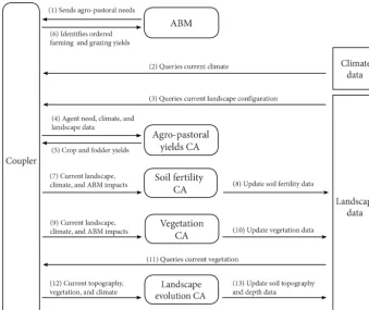
The Mediterranean Landscape Dynamics (MedLanD) project developed a computational laboratory (Bankes et al., 2002) for high-resolution modelling of land-use–landscape interaction dynamics in Mediterranean landscapes called the MedLanD Modeling Laboratory (MML). MML is a virtual lab designed as a configurable and controlled experimental environment to couple representations of human and natural systems (Miller and Page, 2007; van der Leeuw, 2004; Verburg et al., 2016). The MML integrates an agent-based model (ABM) of households practicing subsistence agri-culture and/or pastoralism and cellular automata models of vegetation growth, soil fertility dynamics, and landscape evolution (e.g. erosion/deposition) along with climate scenario data. The components of the MML are connected through a coupler that passes information between them (Fig. 3; Davis and Anderson, 2004, p. 200; Gholami et al., 2014; Sarjoughian et al., 2013, 2015; Sarjoughian, 2006) (see “Approaches to model coupling” section).
900 D. T. Robinson et al.: Modelling feedbacks between human and natural processes in the land system
Figure 3.Structure of feedback between the components of the MedLanD Modeling Laboratory, comprising an agent-based model (ABM), several cellular automata (CA) models, data, and a coupler. Numbers indicate the sequence of steps in a single time step of a coupled model run.
The landscape evolution model (LEM) iteratively evolves digital terrain, soil, and vegetation on landscapes within a watershed by simulating sediment entrainment, transport, and deposition using a 3-D implementation of the Unit Stream Power Erosion/Deposition (USPED) equation and the Stream Power equation (Barton et al., 2016; Mitasova et al., 2013). The LEM also tracks changes in soil depth and fertility due to cultivation and fallowing. A simple vegetation model simulates clearance for cultivation or removal by graz-ing and regrowth tuned to a Mediterranean 50-year succes-sion interval based on empirical studies in the region (Bonet, 2004; Bonet and Pausas, 2007). Climate parameters can be entered iteratively or statically and may derive from any ex-ternal climate or paleoclimate data or simulation output.
2.1.2 Feedback implementation
The coupling architecture of the MML is highly structured, following a tight coupling scheme that is a hybrid of types shown in Fig. 1d and f. In the MML, a coupler manages much of the interaction with data, but it also coordinates the scheduling and exchange of data among the various subcom-ponent models. The coupler was constructed to query data directly and transform it for use by certain submodels but it also directs subcomponent models to run and independently
retrieve data and produce output files. Coordination by the coupler is achieved through the use of a strict file naming system and the use of a common data format (e.g. spatial data must be in the GRASS geographical information sys-tem – GIS – raster file format (Neteler et al., 2012) and other data in delimited text files). Naming conventions of data files indicate data type, temporality, and data permanence (inter-mediary data versus final data). Two versions of the MML have been developed: one where the coupler is an indepen-dent piece of wrapping software coded in Java (in MML v1; Barton et al., 2015a) and one where the coupler is integrated into the main model codebase (in Python) of a reduced ver-sion of MML (in MML-Lite; Barton et al., 2015b). Subcom-ponent models are also either independent software scripts coded in Python (Landscape components) or in Java (ABM) in the MML v1 or are coded in a monolithic Python codebase in the MML-Lite.
au-tomata (CA) submodel (Fig. 3.4). The Agro-Pastoral Yields CA submodel chooses locations for the various subsistence tasks and calculates yields that are returned in the form of a spatial data layer (i.e. a GRASS GIS raster file). Yields are then passed back to the ABM (Fig. 3.6) to determine the ef-fects of subsistence choices for each household. At this time, the human system waits while several natural processes are simulated. The coupler calls the Soil Fertility CA to update soil characteristics degraded by land use (i.e. farming, graz-ing, or firewood gathering) and climate impacts. The coupler then calls the Vegetation CA to determine the amount of veg-etation regrowth following agent land-use impacts (Fig. 3.9). Both the Soil Fertility and Vegetation CAs directly write out-put in the form of GRASS GIS raster files that are queried by the coupler at the beginning of each time step. Lastly, the coupler calls the landscape evolution model, which updates the land surface based on the new configuration of vegetation and climate data for that year.
The new state of the natural system (i.e. altered land sur-face, vegetation, and soils) affects household-agent decisions and natural-system processes (i.e. CA submodels) in subse-quent time steps to achieve two-way feedbacks (as in Fig. 2, upper right). It is worth noting, however, that the MML cur-rently only implements climate as a one-way prescribed cou-pling (Fig. 2).
2.2 Loose coupling – effects of residential land management on carbon storage
2.2.1 Model definition and description
To quantify the effects of residential land management on ecosystem carbon, a framework was developed to couple a human decision-making model with the dynamic global vegetation model BIOME-BGC (Robinson et al., 2013a). Our model of the human system, Dynamic Ecological Exur-ban Development (DEED) model, combines a suite of com-ponents developed to systematically incorporate additional data and complexity in the residential development land-scape (Brown et al., 2004, 2008; Brown and Robinson, 2006; Robinson and Brown, 2009; Robinson et al., 2013a; Sun et al., 2014). Farmer agents own land that is bid on by resi-dential developer agents. The winning resiresi-dential developer agent subdivides the farmland into one of three residential subdivision types, each with different lot density and land-cover impacts (remove all vegetation, leave existing vege-tation, grow new vegetation). Residential household agents then locate and conduct land management activities.
BIOME-BGC was used to represent deciduous broadleaf forest and turfgrass (i.e. maintained lawn) growth. It oper-ates on a daily time step and reports outputs at daily and an-nual periods. Although the model was not developed to in-clude land management, it was selected because (1) existing variables permit the representation of different types of veg-etation found in exurban landscapes (Robinson, 2012) like
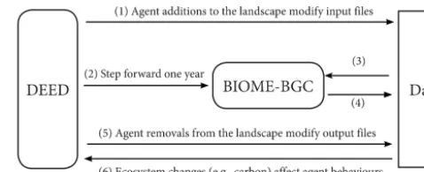
Figure 4.Structure of feedback between DEED and BIOME-BGC. Numbers indicate the sequence of steps in a single time step of a coupled model run. (3) BIOME-BGC retrieves site-characteristic and climate data as well as initial conditions for the next time step comprising biogeochemical pool values among other information. (4) Results of vegetation growth and changes to biogeochemical pools are written back for manipulation by the ABM.
turfgrass (Milesi et al., 2005); (2) the parameters and data used by the model can be altered to represent the impacts of land management that affect vegetation growth; (3) the bio-geochemical cycling in the model represents water, carbon, and nitrogen with extensive literature validating model out-comes, including parameterization for different ecosystems and species (White et al., 2000); and (4) it has been applied both at high spatial resolutions (e.g. 30 m) and at local-to-global spatial extents (e.g. Coops and Waring, 2001), which facilitates both the local site evaluation and the potential to scale out to regional or national levels.
2.2.2 Feedback implementation
A loose coupling approach linking the ABM (DEED) and BIOME-BGC was used that is similar to the structure of Fig. 1c, whereby information is exchanged between data files. However, DEED not only modifies data files used by BIOME-BGC but it also coordinates its run time (Fig. 5). Through this approach, DEED is an independent model and a coupler coordinating interaction with BIOME-BGC.
By chaining the input and output between the two mod-els, two-way feedback is represented (Fig. 2). First, land exchange, land-use change, and land management activi-ties are conducted by agents in DEED. If agents irrigate their property then DEED modifies precipitation values in the climate files used by BIOME-BGC for that year and lo-cation. If agents fertilize, then DEED alters the soil min-eral nitrogen in the BIOME-BGC initial conditions/restart file (Fig. 4.1). Then, DEED steps BIOME-BGC forward by 1 year (Fig. 4.2).
902 D. T. Robinson et al.: Modelling feedbacks between human and natural processes in the land system
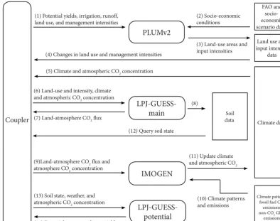
Figure 5.LPJ-GUESS, IMOGEN, and PLUMv2 model coupling structure and feedback between models and data. Numbers indicate se-quence of steps after initialization. (8) LPJ-GUESS-main modifies the soil state locational data.
(e.g. carbon) for a given cell, residential property, or land-scape. Feedback from the ecological system on agent be-haviour was explored through changes in policies that sup-port offset payments for increased carbon storage. An alter-native feedback could include effects on social preferences and norms for landscape design elements (e.g. xeriscaping or adding tree cover) that may drive changes in land manage-ment activities and subsequent ecological outcomes.
2.3 Loose coupling with coupler – changes in food consumption and trade with land-use decisions 2.3.1 Model definition and description
To explore the interactions among land-use decisions, food consumption and trade, land-based emissions, and climate at a global scale, a dynamic global vegetation model (LPJ-GUESS; Smith et al., 2014), a land use and food system model (PLUMv2; Engström et al., 2016), and a climate em-ulator (IMOGEN; Huntingford et al., 2010) were coupled (Fig. 5). Key objectives were (a) to represent the trade-offs and responses between agricultural intensification and expansion and the cross-scale spatial interactions driving system dynamics (Rounsevell et al., 2014), (b) to explore
Economic and behavioural aspects for country-level de-cisions within the food system were modelled in PLUMv2, extending Engström et al. (2016). The PLUMv2 model projects demand for agricultural commodities based on socio-economic scenarios (e.g. shared socio-economic path-ways (SSPs); van Vuuren and Carter, 2014) and attempts to meet these demands through country level cost minimization, including spatially specific land-use selection among other processes such as trade and policy.
2.3.2 Feedback implementation
The coupling of IMOGEN, PLUMv2, and LPJ-GUESS is performed using a coupling script written in CRAN R (R Core Team, 2013), which coordinates data, settings files, and the order of operations for the three models similar to Fig. 1d. The coupling script first performs initialization steps, which produces the required start files and spins up all the models. As part of this process, IMOGEN is spun-up first (Fig. 5). IMOGEN provides spin-up climate for LPJ-GUESS and then PLUMv2. Two instantiations of LPJ-GUESS are used, one for simulated land-use conditions (LPJ-GUESS-main) and one for generating potential crop yields under a range of land uses (LPJ-GUESS-potential).
The coupling script communicates with the IMOGEN and LPJ-GUESS at a 1-year time step, although LPJ-GUESS and IMOGEN operate on sub-daily time steps. IMOGEN is called to provide the climate for the current run year (Fig. 5.9, .11), which LPJ-GUESS-main uses (Fig. 5.5) to simulate the vegetation dynamics with the climate from IMOGEN and the land use from PLUMv2 for the same year (Fig. 5.3, .4, .6)). The terrestrial carbon flux data are aggre-gated to provide global net ecosystem exchange of carbon for the land area with prescribed ocean carbon uptake to IMO-GEN, which estimates the global CO2concentration and cli-mate for the next year.
Every fifth year, the R coupler runs a second instantiation of LPJ-GUESS (LPJ-GUESS-potential), directing it to use the ecosystem soil state of LPJ-GUESS-main (Fig. 5.12, .13). The LPJ-GUESS-potential model is used to produce po-tential net primary production (NPP) for pasture grasslands and potential crop yields for six crop management settings (three levels of fertilization (0, 200, 1000 kg N ha−1) and rain fed or irrigated crops). To account for short-term land-use change legacy effects, LPJ-GUESS-potential uses the previ-ous 10 years of soil conditions and climate from IMOGEN. The last 5 years of the LPJ-GUESS-potential pasture NPP and crop yields are averaged by the R coupler and input to PLUMv2 (Fig. 5.1) to model land use for the next 5-year it-eration. PLUMv2 uses these yield potentials to simulate an-nual land-use management decisions, which are used (as de-scribed above) in the LPJ-GUESS-main model (Fig. 5.4, .6). The land uses are determined using yield potentials for previ-ous time periods in LPJ-GUESS-potential and therefore has been indicated as step 1 in Fig. 5.
2.4 Tight coupling via a coupler – investigating the effects of changes in land use and the energy system on terrestrial and climateCO2 2.4.1 Model definition and description
The integrated Earth System Model (iESM v1.0; Collins et al., 2015a) couples the Global Change Assessment Model (GCAM, v3.0; Wise et al., 2014) with the Community Earth System Model (CESM, v1.1.2; Hurrel et al., 2013) and the Global Land-use Model (GLM, v2; Hurtt et al., 2011) to explore feedbacks between terrestrial ecosystems (includ-ing their interactions with the climate system) and human land use and energy systems. GCAM is an integrated assess-ment model that represents both human and biogeophysical systems (Wise et al., 2014), and in the iESM the climate and carbon components of GCAM are replaced by CESM. The human components simulate global energy and agricul-ture markets to estimate anthropogenic emissions and land change. The energy and land components are distinct but connected via bioenergy, nitrogen fertilizer, and (where ap-plicable) greenhouse gas emissions markets. GLM generates annual, gridded land use from periodic, regional GCAM out-puts following the Land Use Harmonization protocol (LUH; Hurtt et al., 2011), and an additional land-use translator con-verts GLM outputs to CESM land-cover types (Di Vittorio et al., 2014; Lawrence et al., 2012).
CESM is a fully coupled Earth-system model with atmo-sphere, ocean, land, and sea ice components, including land and ocean biogeochemistry that exchanges carbon with the atmosphere (Hurrel et al., 2013). The standard resolution of all CESM components in fully coupled mode is nomi-nally 1◦, but the land cover is determined as fractions of half-degree grid cells and prescribed prior to a simulation (Lawrence et al., 2012). Biogeographical vegetation shifts are not included, although ecosystems do respond and con-tribute to changing environmental conditions. The CESM land model includes detailed hydrology and mechanistic veg-etation growth for 16 plant functional types (PFTs) to simu-late water, carbon, and energy exchange with the atmosphere. The iESM coupling follows the Coupled Model Intercom-parison Project phase 5 (CMIP5; Taylor et al., 2012) LUH protocol (Hurtt et al., 2011), with some modifications and ad-ditions (Bond-Lamberty et al., 2014; Di Vittorio et al., 2014), to connect GCAM and GLM (Hurtt et al., 2011) directly to the CESM framework via a newly developed integrated as-sessment coupler (Collins et al., 2015a).
2.4.2 Feedback implementation
904 D. T. Robinson et al.: Modelling feedbacks between human and natural processes in the land system
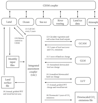
Figure 6.Structure of iESM and feedback between integrated model components. An integrated assessment coupler facilitates all inter-actions between the Global Change Assessment Model (GCAM), the Global Land-Use Model (GLM), and the Community Earth System Model (CESM). The coupler is activated by the CESM land model every 5 years to calculate the average carbon and productivity scalars for the past 5 years and pass them to GCAM, then pass GCAM outputs to the atmosphere component of CESM via a downscaling algorithm and to GLM, and then pass GLM outputs to the land component via a land-use translator (LUT). The non-CO2emissions are provided to CESM as an input data file.
This coupler coordinates communication between the human and environmental systems by first calculating average crop productivity and ecosystem carbon density scalars from the previous 5 years of CESM net primary productivity and het-erotrophic respiration outputs (Bond-Lamberty et al., 2014), except during the initial year when these scalars are set to unity (Fig. 6.2). The coupler then runs GCAM with these scalars to project fossil fuel CO2 emissions and land-use change for the next 5 years (Fig. 6.3), and then passes these outputs through downscaling algorithms to the atmosphere and land components of CESM (Fig. 6.4–.9). The non-CO2 emissions are prescribed by CMIP5 data as initial CESM in-put files. Land-use change is annualized and downscaled by GLM (Hurtt et al., 2011) (Fig. 6.4, .5). A land-use transla-tor converts these changes in cropland, pasture, and wood-harvested area into changes in CESM land-cover change, which is based on plant functional types (Di Vittorio et al.,
2014, Lawrence et al., 2012) (Fig. 6.6, .7). The CO2 emis-sions are downscaled following Lawrence et al. (2011) and passed to the atmosphere component as a data file (Fig. 6.8), and the land-cover change is stored in a land surface file and passed to the land component (Fig. 6.9). The coupler then re-turns control to the land model and CESM runs for another 5 years (Fig. 6.10). This two-way feedback incorporates the effects of climate change, CO2fertilization, and nitrogen de-position on terrestrial ecosystems into GCAM’s projections.
enables feedbacks by running GCAM, GLM, and a new land-use translator inline with CESM.
These capabilities enable new insights into research ques-tions regarding climate mitigation and adaptation strategies. For example, how may agricultural production shift due to climate change, how do different policies influence this shift, and how may this shift affect other aspects of the human– Earth system? Many recent impact studies (e.g. ISIMIP, BRACE, CIRA2.0) use climate model simulations based on emissions and land-use scenarios (Representative Concentra-tion Pathways, RCPs) that themselves do not account for the influence of climate change on future land use. This inconsis-tency could affect conclusions about impacts resulting from particular RCPs.
This approach paradoxically has several strengths that are also weaknesses. The main strength of this approach is that it tightly couples two state-of-the-art global models to imple-ment primary feedbacks between human and environimple-mental systems under global change. Unfortunately, this configura-tion is not amenable to the uncertainty and policy analyses or the climate target experiments usually employed by GCAM because it takes too long to run a simulation. As a global model it provides a self-consistent representation of intercon-nected regional and global processes, both human and envi-ronmental, but is unable to capture a fair amount of regional and local detail that influences planning and implementation of adaptation and mitigation strategies.
3 Discussion
The four presented examples demonstrate how specialized models of human and natural processes have been connected through alternative coupling approaches to address research questions related to the impacts of one system on another and the effects of feedbacks between human and natural sys-tems on a variety of outcomes of interest (e.g. erosion, carbon storage, and emissions). The focus on specialized models of-fers a flexible and open approach to answering new questions about feedbacks in coupled human–natural systems and also facilitates the identification of new types of data required to calibrate and validate the interactions and feedbacks between the two systems. Additionally, coupled modelling presents an opportunity for increased transparency and detail in the rep-resented processes through more explicit identification and documentation of component interactions and processes.
The example models are diverse in the spatial and thematic resolutions of human- and natural-system processes repre-sented. The first two examples (MML and DEED) use agent-based approaches that represent land use and land manage-ment in the human system at the household level. While the ecological impact of land management activities in DEED does not have a direct feedback on residential household decision making, those represented in MML do. Agricul-tural systems, carbon markets, and policies provide
mech-anisms to establish this feedback and endogenize the impact-response cycle between residential land management prac-tices of the human system and the natural system (Sun et al., 2014).
The second two examples are global models with differ-ent levels of coupling and complexity that represdiffer-ent human– natural-system feedbacks at regional and global levels. In both examples, the human system has a direct effect on mod-elled natural-system processes (i.e. vegetation, carbon, cli-mate), and the feedback of environmental changes on human systems is mediated by vegetation responses to changing nat-ural and human conditions.
These examples demonstrate how coupled system imple-mentations extend the applicability of models to a variety of questions regarding the dynamic relationship between human and environmental systems that would otherwise be impos-sible to address quantitatively. Such questions include those related to direct and indirect effects of one system on an-other (e.g. what is the effect of the natural system on the human system?), to the resilience or sensitivity of the cou-pled system or its components to perturbations or scenarios (e.g. do feedbacks dampen or amplify the consequences of a perturbation?), and to identifying thresholds (e.g. what is the critical value of a variable in one system that when crossed instantiates change in the other system?), among many oth-ers.
3.1 Lessons learned
To make progress in modelling coupled human–natural sys-tems, the way in which some set of variables or processes affects or interacts with both systems must be specified. For example, precipitation has a known and direct effect on plant growth (e.g. forest or crop) and erosion (e.g. overland flow). The outcomes of some of these processes (e.g. yield and soil loss) have direct or indirect effects on land management choices by farmers, effects that are empirically observable at least qualitatively and, in some instances, quantitatively measured. However, the direct impacts of other perturba-tions, such as the introduction of new technology or gov-ernance schemes, on human- and natural-system processes are not observable because they have not yet occurred. The presented case studies focus on perturbations or scenarios that are grounded in known and direct causal relationships that are more likely to be found in the natural system than the human system, partly due to the multitude of drivers affecting—and consequent difficulty in predicting—human-decision making. In these example cases, a number of lessons have been learned:
906 D. T. Robinson et al.: Modelling feedbacks between human and natural processes in the land system
range of parameters and use of simulated data or expert-or theexpert-ory-infexpert-ormed methods to evaluate the relative con-tribution of parameter values/ranges, missing data, or processes on model outcomes. For example, to properly understand the net effect of human alteration to vegeta-tion on long-term rates of erosion and deposivegeta-tion in the MML, it became clear that a more complete understand-ing of the sensitivity of the landscape evolution subcom-ponent model to vegetation was needed. This sensitivity analysis showed a very strong exponential relationship between vegetation type and both the overall amount of erosion and deposition over time and the temporal vari-ation in erosion rates over time (Ullah, 2017), The anal-ysis show a particular sensitivity to expanded bare land, grasslands, and shrub land-cover types. Therefore, it is clear that agent activity that leads to an increase these types of land cover should also lead to long-term in-creases in erosion and deposition in the MML. In this way, model sensitivity to parameters, data, or processes can be evaluated to support design and deployment of resources for new data collection.
– Lesson 2: modelling is an iterative process. The pro-cess of analyzing coupled human- and natural-system models often results in the identification of needs to in-vestigate key variables, data, or mechanisms. For exam-ple, through the coupling of DEED and BIOME-BGC (Sect. 2.2), it was realized that data on vegetation and soil carbon for residential land uses are grossly inad-equate for model calibration. This realization fostered new data collection and analysis about the distribution of carbon stored in different residential land uses (Cur-rie et al., 2016). New forms of measurement and eval-uation are often needed to collect novel data and quan-tify variables and feedbacks linking human and natural systems. As these new data are collected and become available, new questions about model processes are in-evitable (Rounsevell et al., 2012).
– Lesson 3: create a common language.Coupling human and natural systems brings social and natural scientists together that often have a different understanding of the meanings of commonly used terms. Both technical and conceptual aspects of the coupling process can be im-proved when a common language is used. For example, traditional coupling between the ocean and the atmo-sphere in Earth-system models typically uses the cli-mate and forecast conventions (Eaton et al., 2011). A controlled vocabulary in these conventions assists the understanding of model processes and facilitates their coupling among models or replacement in new mod-els. With a similar goal but different approach, CSDMS introduced rules for the creation of unequivocal terms through their standard names system that function as a semantic matching mechanism for determining whether two terms refer to the same quantity with associated
predefined units. This concept is currently undergoing transition to a geoscience standard names ontology that reaches out to include social science terms (David et al., 2016), which can benefit communication between com-munities (i.e. natural and social science) that may have different terms and descriptions of similar processes (Di Vittorio et al., 2014). With a common language, data can be more easily and unambiguously communicated between components in a coupled system.
– Lesson 4: make code open-access. Many ecosystem and Earth-system models have mass, energy, or other balance equations that constrain the processes to the laws of thermodynamics and can be used to ensure that they are working correctly. For example, the ecosys-tem model LPJ-GUESS has a routine to ensure bal-ance between influx, efflux, and storage of carbon. Sim-ilar checks and balances are used in human-system models with respect to population change (e.g. births, deaths, immigration, and emigration) or economic trade (e.g. production, consumption, imports, and exports) at macro levels and budget or labour constraints at house-hold or individual levels. However, in many natural-system models these balance equations are not acces-sible for coupling and the representation of human per-turbations and modifications to the factors in balance equations are either not included or done so indirectly and make the coupling less flexible and tractable. Mov-ing forward, critical equations, like mass balance equa-tions, and model variables should be made open through coding to provide multiple points for interfacing with other models (specifically human-systems models).
– Lesson 5: ensure consistency.Modelers seeking to cou-ple natural- and human-systems models that represent similar phenomena, like land cover, can encounter sig-nificant ontological and process consistency challenges. Models with different initial assumptions and different processes can generate different values for the same phenomenon. While model coupling can ultimately pro-vide an impetus for harmonizing and resolving such consistency issues, it requires decisions about which processes to represent and which to leave out to avoid duplication.
harvest was conceptually different across the three mod-els comprising iESM (GCAM, GLM, and CESM), with each model having its own process for determining how harvest is spatially distributed. Wood harvest is a good example of different modelling groups describing the same thing and using the same language but with very different concepts and processes, with unintended con-sequences for CESM’s terrestrial carbon cycle.
– Lesson 6: reconcile spatio-temporal mismatch. Many natural-system models operate at finer temporal and coarser spatial resolutions than human-system models (Evans et al., 2013). Often, these discrepancies cannot simply be dealt with by aggregation of the variables be-cause they represent mismatch in spatial and temporal dynamics that may also happen in reality. Human re-sponses to environmental change may show significant time lags or may be related to cycles of management (e.g. cropping cycles) rather than showing an immedi-ate response. Similarly, while the ecological models are strongly place-based, coupling human and natural sys-tems at the pixel level may not always be appropriate due to complex spatial relations in the human dimen-sions (e.g. distant land owners) or responses across dif-ferent levels of decision making (e.g. policy responses) that are not linked to the exact place of the ecological impact. Reconciling these mismatches involves balanc-ing detail and computational tractability within existbalanc-ing model structures and scheduling the frequency of com-munication between models.
As an example, the DEED ABM (Sect. 2.2) used an annual time step to reflect the timing of land manage-ment decisions, whereas the ecosystem model BIOME-BGC represented vegetation growth and biogeochemi-cal cycles daily. To reconcile these differences, irriga-tion decisions were made annually but implemented 1 day a week during the growing season by modifying the daily precipitation file used by BIOME-BGC. In con-trast, other management activities were implemented once annually before (for fertilization) and after (for removals) the growing season. These limitations could have a significant effect on estimated carbon storage and have fostered additional fieldwork for further validation (e.g. Currie et al., 2016) and additional efforts to tightly couple the two models.
The iESM (Sect. 2.4) also reconciles similar mis-matches through a 5-year time lag and specialized spa-tial and temporal downscaling of economic model out-puts to provide inout-puts to the environmental model. While these approaches allow the separate models to operate synchronously, further development to better match the inherent spatio-temporal configurations be-tween models is required to reduce errors associated with such mismatches.
– Lesson 7: construct homogeneous units.Coupling mod-els increases computational overhead and thus requires increases in computational efficiency, both of which come with trade-offs. One approach to improving ef-ficiency is to classify and generalize components of the model such as agent types in the human system (e.g. Brown and Robinson, 2006), types of vegetation (e.g. plant functional types, Díaz and Cabido, 1997; Smith et al., 1993, 1997), or landscape units. Landscape units are not typically constructed to structure spatial vari-ability in land-use science, but are used regularly in hy-drological modelling; for example, the Soil Water As-sessment Tool (SWAT; Neitsch et al., 2011) uses hy-drological response units (HRUs) that have a soil pro-file, bedrock, and topographic characteristics that are as-sumed to be homogeneous for the entire spatial extent of the unit. Similar concepts have been used to iden-tify management zones or units, and our examples of DEED-BIOME-BGC (Robinson et al., 2013a) and the iESM (Collins et al., 2015a) both employed this ap-proach. However, the variability among management activities and land-cover types can lead to a large com-bination of outcomes, and the delineation of these units directly contributes to uncertainty in model projections (Di Vittorio et al., 2016).
– Lesson 8: incorporating feedback increases non-linearity and variability.Specific results from the four examples are available in a number of publications asso-ciated with each example. Among the four example cou-pling efforts, it has been found that the incorporation of two-way feedbacks (Fig. 2) between models of the hu-man and natural system typically produces non-linear results and a greater range in model outcomes than are observed when the models are isolated or one-way pre-scriptions are used. For both the MML and DEED mod-els, changes in the natural system were relatively linear when one-way human perturbations were prescribed. However, when feedbacks between the systems were in-corporated then non-linear outcomes and frequently a greater variation in model outcomes were observed.
3.2 Feedback effects
ecosys-908 D. T. Robinson et al.: Modelling feedbacks between human and natural processes in the land system
tem productivity could change due to atmospheric influences (e.g. climate change, CO2fertilization) or to terrestrial influ-ences associated with changing ecosystem area (e.g. spatially heterogeneous soil properties, changes in the proportion of different forest types). Regardless of the challenges, an over-all benefit of quantifying feedback effects is that modellers can gain insight into processes that are typically not observed and measured. Given the difficulty in observing these effects and potential inconsistencies, efforts in coupling human- and natural-system models have focused on sensitivity analysis to test their effects (e.g. Harrison et al., 2016).
Ultimately, an important goal in such analyses is to discern which of two distinct sources produce effects from includ-ing feedbacks in coupled models: (1) model implementation (both technical and conceptual) and (2) the actual feedback signal. Model implementation issues often relate to the level of consistency between the original models. For example, the need to translate changes in gridded patterns of ecosystem productivity to changes in regional average carbon density can lead to varying sensitivities across magnitudes of produc-tivity and areal change, requiring the unrealistic sensitivities to be filtered out (Bond-Lamberty et al., 2014).
Model experiments are useful for separating the model im-plementation issues from the actual feedback signal. For ex-ample, iESM was used in a series of land-only simulations to (a) quantify the relationship between ecosystem productiv-ity and carbon densproductiv-ity, (b) implement a statistical method to remove outliers that introduce error due to extreme combina-tions of land cover and productivity change, and (c) develop the appropriate proxy variables for use by GCAM (Bond-Lamberty et al., 2014). To verify that this process effectively removed the model implementation effects, another series of land-only simulations was conducted using the iESM with and without terrestrial feedbacks and with constant atmo-spheric conditions (i.e. year 1850 aerosols and nitrogen de-position, and repeating 15 years of climate forcing). This ex-periment showed that the coupling itself, without an atmo-spherically driven feedback signal, did not generate signifi-cant changes in GCAM outputs. The feedback signal was not zero, however, indicating that a combination of implementa-tion effects and land heterogeneity effects was present. These combined effects were not separable due to lack of data on the required outputs, and in general they were opposite to the total feedback effects in the fully coupled iESM experiment, suggesting that the atmospherically driven feedbacks may be larger than the net feedbacks.
Depending on the mechanisms involved, feedbacks may create strong feed-forward effects that lead to a fast evolu-tion of the dynamics of the system. By contrast, responses may also lead to an attenuation of perturbations and strong stability of the dynamics. Where the exact mechanisms in-volved and the strength of the feedbacks are unknown, model dynamics may start deviating strongly upon small changes in variable settings, in other words, leading to strong model sensitivity to highly uncertain model parameters.
The examples including feedbacks in coupled human– natural-system models illustrate a number of challenges in designing and implementing feedback mechanisms:
– The representation of human responses. The exam-ples in the four cases above mostly relate to a cou-pling based on exchanging land-cover and ecological-process-impact information. The human decision mod-els translate the ecological impacts to alter decision making. For example, land-use decisions in PLUM-LPJGUESS, iESM, and MedLanD respond to changes in potential yields; in the MedLanD application, erosion processes also render land less suitable for use. In real-ity the responses of human decision making are more complex. The relevance of the ecological indicator ex-changed may be context dependent; e.g. potential yields may determine farming decisions in capital intensive farming that is near to the production frontier but may be much less important in low-input subsistence farm-ing that is far from potential productivity. Furthermore, decision making may not be based on the represented process or the indicator exchanged but rather on the human perception of the environmental change, which may be irrational and biased by other interests, such as in the case of the climate debate. While the concept of environmental cognitions is well known, relatively little is known in relation to land-use change decision making (Meyfroidt, 2013a). Human responses to environmental change are, therefore, a critical knowledge gap for im-plementing coupling mechanisms (Meyfroidt, 2013b).
– Structural differences in model concepts. The iESM ex-ample illustrates how structural differences in models can hamper the coupling of models, and how careful consideration is needed of the feedback mechanism and its consequences in relation to the overall model as-sumptions. This is especially relevant for coupling mod-els that assume equilibrium and those that depict in-stantaneous impacts or transient situations. Global eco-nomic models using equilibrium assumptions, which are frequently coupled to land-use and ecosystem mod-els and specialized land-change modmod-els (or land-change modules in IAM models) both address land use but of-ten from different perspectives leading to poof-tential dif-ferences in the meaning and interpretation of input and output variables.
mod-els (especially econometric style modmod-els). Other modmod-els have algorithms that generate stochasticity to represent uncertainty in processes. Many agent-based/individual-based models and some cellular automata fall into this category. For models with included stochasticity, the same random number generator seed can be used; how-ever, to capture the variance and distribution of model outcomes, repeated runs with different seeds are re-quired, which can be conceptually challenging or oper-ationally complicated when coupled with deterministic models.
3.3 A way forward
The ability to dynamically simulate feedbacks between hu-man decision making and natural processes requires some kind of tight coupling – in the sense of frequent, two-way communication and high coordination (Fig. 2) – between models designed to represent these different processes. To date, this has largely been achieved through connecting mod-els into a single modelling environment. This is true to a large extent for all the case studies presented here. Adding new models to such systems often requires significant reprogram-ming and makes the expanded code base increasingly dif-ficult to debug, verify, and validate. Additionally, any other researcher that would like to combine fewer, more, or dif-ferent components will need to reprogram multiple parts of the modelling environment to decouple one model and add another.
To expedite coupling in future modelling of the land sys-tem, we recommend a bottom–up approach to modelling whereby modelers with in-depth domain knowledge create relatively small, more easily verified modules (Bell et al., 2015) or model components for assembly into larger cou-pling frameworks (e.g. OpenMI, ESMF, OMS, and CSDMS). Using this approach, the community may preserve and build upon existing numerical code previously developed by the many subdisciplines involved in modelling human and nat-ural systems. These are not new ideas, but they have not yet been achievable in spite of their recognized desirability. However, a suite of technologies has reached sufficient ma-turity that it may now be a practical way to create a new gen-eration of modelling tools that can exploit these two avenues for modelling coupled human–natural systems.
New coordinating frameworks for next generation cou-pled modelling of human and Earth systems are being de-veloped within a number of relevant organizations: the CS-DMS, the Network for Computational Modeling in Social and Ecological Sciences (CoMSES Net), and the Analysis, Integration, and Modeling of the Earth System (AIMES) Core Project of Future Earth. These frameworks envision a set of community-developed and endorsed standards for open, platform-independent model coupling and integration based around an interrelated set of components that build on lessons 3–6.
– Start with wrapper container software (e.g. Docker) to encapsulate model code and dependencies needed.
– Use a standardized API, like the extension of the Basic Modeling Interface (BMI) developed by the CSDMS, to standardize and describe various functions (e.g. model control, model information, time, variable information, variable getters and setters, and model grids) such that a calling component in the framework is provided with the level of control needed to access other component’s metadata and simulated data (Hutton et al., 2014).
– Incorporate Standard Names to map variables of mul-tiple components to each other. In the CSDMS frame-work the Standard Names functions as a semantic matching mechanism, a lingua franca, for determining whether two variable names refer to the same quantity with associated predefined units.
– Mitigate sunk-cost effects for integration into any one coupling framework by creating separate interfaces to one or more coupling frameworks (Peckham et al., 2013; Lemmen et al., 2018a).
– Adopt reproducible workflow environments to wire models together, supervise their execution and manage the storage of the intermediate and final results needed for subsequent analysis.
910 D. T. Robinson et al.: Modelling feedbacks between human and natural processes in the land system
4 Conclusions
Coupling human-system and natural-system models requires connecting distinct research fields, each with unique knowl-edge, methods, assumptions, definitions, and language. Suc-cess depends on the research team members learning enough about the other field and model to unambiguously commu-nicate with each other, recognize strengths and weaknesses of other methods, translate assumptions and definitions, and critically evaluate other model processes and outputs. Ad-ditionally, some team members need to develop working expertise of both models and fields to facilitate the imple-mentation of an internally-consistent coupled model. Fur-thermore, a software engineer is often needed to address the technical challenges of coupling complex models. Ulti-mately, the social and conceptual challenges combine to re-quire much more time and effort for successful completion than for similar, mono-disciplinary projects. Nonetheless, all authors noted that the greatest benefit of the coupling process was the collaborative learning process that created a group of people with a working knowledge of both human- and natural-system research and expertise in how to integrate the two.
While successful coupling of human- and natural-systems models requires truly interdisciplinary collaboration, we note that the playing field is not level with respect to disciplines. There are more resources and active modelling efforts in the natural sciences than in human-systems science. This is un-fortunate since natural scientists need to closely work with human-systems scientists to understand the kinds of informa-tion needed and the kinds of informainforma-tion that can be provided by models of human systems. Moreover, the most scientifi-cally and socially valuable results of model coupling require that both natural-systems models and human-systems models be modified and enhanced to work together. The collabora-tive model development that this entails involves social inter-actions, two-way communication, and mutual respect for do-main knowledge as well as technical solutions. In this regard, there needs to be scientific, professional, and policy incen-tives for all members of the interdisciplinary teams needed to develop successful integrated modelling.
These efforts highlight the difficulty and challenges asso-ciated with the process of human–environment model cou-pling as well as the opportunities that coucou-pling presents for making substantive and methodological advances in science associated with human systems, natural systems, and their feedbacks on each other.
Data availability. The underlying models and frameworks dis-cussed in the presented research can be found through the URLs and DOIs provided below. The range of documentation and support for each model or framework varies. It should be assumed upon down-loading that no support is available. While the posting of these mod-els promotes transparency, their creation has involved teams of
in-dividuals who hold extensive experience and tacit knowledge work-ing with the models and frameworks. The authors caution against their use and evaluation for scientific results without collaboration or consultation with their developers or members of their research teams.
The MedLanD Modeling laboratory can be referenced as Barton et al. (2018). The DEED conceptual model can be cited as Robinson et al. (2013a) with code retrieved from Robinson et al. (2013b). The PLUMv2 conceptual model can be cited as Alexander et al. (2018) with code retrieved from Alexander and Henry (2018). The LPJ-Guess conceptual model can be cited as Smith et al. (2014) and code requested from the authors. The iESM conceptual model can be cited as Collins et al. (2015b), with Version 1 code retrieved from Collins et al. (2015b). The CSDMS standards (CSDMS Integration Facility, 2018a), framework (CSDMS Integration Facility, 2018b), and software and model repositories (CSDMS community contribu-tion) are made available on github. The MOSSCO model coupling framework can be retrieved from Lemmen et al. (2018b).
Competing interests. The authors declare that they have no con-flict of interest.
Special issue statement. This article is part of the special issue “Social dynamics and planetary boundaries in Earth system mod-elling”. It is not associated with a conference.
AGS-1243095. Peter H. Verburg was supported by the European Union’s Seventh Framework Programme ERC grant agreement no. 311819 – GLOLAND.
Edited by: Jonathan Donges
Reviewed by: three anonymous referees
References
Alexander, P. and Henry, R.: PLUMv2, https://bitbucket.org/ alexanpe/plumv2/src/RCPpaper, last access: 18 June 2018. Alexander, P., Rabin, S., Anthoni, P., Henry, R., Pugh, T. A. M.,
Rounsevell, M. D. A., and Arnet, A.: Adaptation of global land use and management intensity to changes in climate and at-mospheric carbon dioxide, Global Change Biol., 7, 2791–2809, https://doi.org/10.1111/gcb.14110, 2018.
Bai, X., van der Leeuw, S., O’Brien, K., Berkhout, F., Biermann, F., Broadgate, W., Brondizio, E., Cudennec, C., Dearing, J., Du-raiappah, A., Glaser, M., Steffen, W., and Syvitski, J. P.: Plausi-ble and DesiraPlausi-ble Futures in the Anthropocene, Global Environ. Change, 39, 351–362, 2015.
Bankes, S. C., Lempert, R., and Popper, S.: Making Computational Social Science Effective: Epistemology, Methodology, and Tech-nology, Social Sci. Comput. Rev., 20, 377–388, 2002.
Banning, E. B.: Houses, households, and changing society in the Late Neolithic and Chalcolithic of the Southern Levant, Paleori-ent, 36, 46–87, 2010.
Barton, C. M., Ullah, I. I., Mayer, G. R., Bergin, S. M., Sarjoughian, H. S., and Mitasova, H.: MedLanD Modeling Laboratory v.1, CoMSES Computational Model Library, https://www.openabm. org/model/4609/version/1 (last access: 8 May 2015), 2015a. Barton, C. M., Ullah, I., and Heimsath, A.: How to Make a
Bar-ranco: Modeling Erosion and Land Use in Mediterranean Land-scapes, Land, 4, 578–606, https://doi.org/10.3390/land4030578, 2015b.
Barton, C. M., Ullah, I. I. T., Bergin, S. M., Sarjoughian, H. S., Mayer, G. R., Bernabeu-Auban, J. E., Heimsath, A. M., Acevedo, M. F., Riel-Salvatore, J. G., and Arrowsmith, J. R.: Experimental socioecology: Integrative science for An-thropocene landscape dynamics, AnAn-thropocene, 13, 34–45, https://doi.org/10.1016/j.ancene.2015.12.004, 2016.
Barton, C. M., Ullah, I., Mayer, G., Bergin, S., Sarjoughian, H., and Mitasova, H.: MedLanD Modeling Laboratory v.1 (Ver-sion 1.1.0), CoMSES Computational Model Library, https: //www.comses.net/codebases/4609/releases/1.1.0/, last access: 13 June 2018.
Bell, A. R., Robinson, D. T., Malik, A., and Dewal, S.: Modular ABM development for improved dissemina-tion and training, Environ. Model. Softw., 73, 189–200, https://doi.org/10.1016/j.envsoft.2015.07.016, 2015.
Bonan, G. B.: A Land Surface Model (LSM Version 1.0) for Eco-logical, HydroEco-logical, and Atmospheric Studies: Technical De-scription and User’s Guide, NCAR Technical Note NCAR/TN-417+STR, National Center for Atmospheric Research, Boulder, Colorado, https://doi.org/10.5065/D6DF6P5X, 1996.
Bond-Lamberty, B., Calvin, K., Jones, A. D., Mao, J., Patel, P., Shi, X. Y., Thomson, A., Thornton, P., and Zhou, Y.: On linking an Earth system model to the equilibrium carbon representation of
an economically optimizing land use model, Geosci. Model Dev., 7, 2545–2555, https://doi.org/10.5194/gmd-7-2545-2014, 2014. Bonet, A.: Secondary succession of semi-arid Mediterranean
old-fields in south-eastern Spain: insights for conservation and restoration of degraded lands, J. Arid Environ., 56, 213–233, https://doi.org/10.1016/S0140-1963(03)00048-X, 2004. Bonet, A. and Pausas, J. G.: Old Field Dynamics on the Dry Side
of the Mediterranean Basin: Patterns and Processes in Semi-arid Southeast Spain, in: Old Fields: Dynamics and Restoration of Abandoned Farmland, Island Press, Washington, D.C., USA, 247–264, 2007.
Brown, D. G. and Robinson, D. T.: Effects of heterogeneity in res-idential preferences on an agent-based model of urban sprawl, Ecol. Soc., 11, 46, 2006.
Brown, D. G., Page, S. E., Riolo, R., and Rand, W.: Agent-based and analytical modeling to evaluate the effectiveness of greenbelts, Environ. Model. Softw., 19, 1097–1109, 2004.
Brown, D. G., Robinson, D. T., An, L., Nassauer, J. I., Zellner, M., Rand, W., Riolo, R., Page, S. E., Low, B., and Wang, Z.: Exurbia from the bottom-up: Confronting empirical challenges to charac-terizing a complex system, Geoforum, 39, 805–818, 2008. CSDMS Integration Facility: CSDMS BMI Standards, https://
github.com/bmi-forum (last access: 18 June 2018), 2018a. CSDMS Integration Facility: CSDMS main framework repository,
https://github.com/csdms (last access: 18 June 2018), 2018b. CSDMS community contribution: CSDMS software contributions
of the community, https://github.com/csdms-contrib (last access: 18 June 2018), 2018c.
Collins, W. D., Craig, A. P., Truesdale, J. E., Di Vittorio, A. V., Jones, A. D., Bond-Lamberty, B., Calvin, K. V., Edmonds, J. A., Kim, S. H., Thomson, A. M., Patel, P., Zhou, Y., Mao, J., Shi, X., Thornton, P. E., Chini, L. P., and Hurtt, G. C.: The integrated Earth System Model version 1: formulation and functionality, Geosci. Model Dev., 8, 2203–2219, https://doi.org/10.5194/gmd-8-2203-2015, 2015a.
Collins, W. D., Craig, A. P., Truesdale, J. E., Di Vittorio, A. V., Jones, A. D., Bond-Lamberty, B., Calvin, K. V., Edmonds, J. A., Kim, S. H., Thomson, A. M., Patel, P., Zhou, Y., Mao, J., Shi, X., Thornton, P. E., Chini, L. P., and Hurtt, G. C.: The integrated Earth System Model version 1, https://gitub.com/ ACME-Climate/iESM (last access: 13 June 2018), 2015b. Coops, N. C. and Waring, R. H.: The use of multiscale remote
sens-ing imagery to derive regional estimates of forest growth capacity using 3-PGS, Remote Sens. Environ., 75, 324–334, 2001. Currie, W. S., Kiger, S., Nassauer, J. I., Hutchins, M., Marshall,
L. L., Brown, D. G., Riolo, R. L., Robinson, D. T., and Hart, S.: Human-dominated residential land in southeastern Michigan stores carbon similar to secondary forests, Ecol. Appl., 26, 1421– 1436, 2016.
David, C. H., Gil, Y., Duffy, C., Peckham, S. D., and Venayagamoorthy, S. K.: An introduction to the Earth and Space Science, in: special issue: “Geoscience Pa-pers of the Future”, American Geophysical Union, 1–4, https://doi.org/10.1002/2016EA000201, 2016.
Davis, P. K. and Anderson, R. H.: Improving the Composability of DoD Models and Simulations, J. Defense Model. Simul., 1, 5– 17, https://doi.org/10.1177/154851290400100101, 2004. Deadman, P. J., Robinson, D. T., Moran, E., and Brondizio, E.: