Mathematical Modeling of Acoustic Signals Generated During Gas Tungsten Arc Welding Process

Mathematical Modeling of Acoustic Signals Generated

During Gas Tungsten Arc Welding Process

Kaustubh S. Samvatsar

Production Engineering Department, Birla Vishvakarma Mahavidyalaya, Vallabh Vidyanagar, Anand, Gujarat, India

kaustubhsamvatsar@gmail.com

Abstract—Adoption of alternative advanced approaches for monitoring the ongoing welding can impart a transcendental process-control and can worthily substantiate the regulation of produced weld quality. Acoustic emission analysis, being a highly effective technology has paved way by facilitating the investigation of defects while operation is going on. Essential precise quantification has been carried out for inducing interrelationship of the response variables with the input parameters to predict further behavior of weld and rectification of these process parameters so that unintended defects during gas tungsten arc welding (GTAW) can be minimized. To verify the adequacy and agreeability of designed model, a corroborating evaluation has been performed.

Keywords—acoustic emission; GTAW; regression; prediction; characterization.

I. INTRODUCTION

Acoustic emission analysis is a non-conventional method of non destructive testing which is capable of detecting the generation of defect at the time of welding. Elasticity is an important property of solid materials which allows its compression under the effect of external forces and spring back phenomenon under the removal of these forces. A fracture generates if the elastic limit is exceeded either immediately or after certain plastic deformation. A rapid release of elastic energy occurs from the elastically strained material due to the containment or generation of defects such as non-metallic inclusion, weld joint defect, cracks, etc. This is called as an acoustic emission event. The propagation of elastic wave can be detected using sensitive and most appropriate sensors. The frequency of ultra-sound in an acoustic emission event generally ranges between 100 and 300 KHz and its reliable measurement can be done by short sensor distance in proper laboratory environment. For GTAW, acoustic variation can arise from geometrical or gas flow rate change, metallic transfer, etc. [1] Conjunction of mathematical models with designed experiments can be used for prediction of the magnitude of sound pressure recorded by means of proper arrangement. It can assure sufficient reliability. [2]

II. MATERIALS AND METHODS

Figure 1. Acoustic signals recording

Once the acoustic waves have been recorded, die penetrant test can be performed on the welded area. Then, for detection of internal defects, Radiographic testing and/or Ultrasonic testing can be done. Such a correlation has been found successfully. [1] Acoustic emission produced by metal droplet transfer is due to rapid release of elastic energy when any discontinuity is encountered.

Figure 2. Experimental Set-up[1]

A microphone is firmly supported on a stand which is of unidirectional type. It is capable of recording the signals generated during the welding process. This microphone is connected to a computer on which Trial version of Multi Instrument software shows the fluctuation of acoustic waves on its display screen. The DCEN welding process takes place in synergic mode using Argon as inert gas.The experiments have been conducted by GTAW the work-piece of length 150mm. Figure 2 depicts sectional geometry of the work-piece.

Figure 3. Geometry of work-piece

The chemical composition of work-piece and its mechanical properties with their designation code are mentioned in table I and II respectively as follows.

TABLE I. CHEMICAL COMPOSITION OF WORK-PIECE

Jindal Designation/code %C %Mn %P %S %V %Cr %Ni %Mo %Fe N (ppm)

J-304 L 0.03 1.19 0.05 0.03 0.28 17.93 8.56 0.27 Rest 1000

TABLE II. MECHANICAL PROPERTIES OF WORK-PIECE

Jindal Designation/code

Tensile Strength (MPA)min.

%Yield

Strength(MPA)min % Elongation(min.)

Hardness (HRB) max.

J-304L 485 170 40 95

The chemical composition of filler wire and its mechanical properties with their designation code having diameter Ø1.6mm are mentioned in table III and IV respectively as follows.

TABLE III. CHEMICAL COMPOSITION OF FILLER WIRE

Electrode code %C %Mn %Si %Cr %Ni %Mo %Fe ER-316L 0.02 1.50 0.40 19.00 12.00 2.0 Rest

TABLE IV. MECHANICAL PROPERTIES OF FILLER WIRE

Electrode

code Process

Tensile Strength (N/mm2₎

Impact J (RT)

Recommended flux

Melting Point (°C)

Hardness (HRB)

Welding Conditions

ER-316L TIG & Gas 590 60 Stainless Steel 1440ºC 180 DC+, AC

TABLE V. MICROPHONE SPECIFICATIONS

Manufacturer Directivity

Frequency Response

(Hz)

Output Impedance

Sensitivity (dB)

Dimensions (mm)

Mass (g)

Cord Length (m)

SONY Ltd, Japan Unidirectional 60-12000 600 in 1kHz Ω -53.0 Ø51 x 204 140g 3

On a Gas Tungsten Arc Welding machine, various modes for welding are available. Experimentation has been carried out for test bead and visual examination has been performed. It can be observed from figure 3 that the weld test bead produced in synergic mode as compared to other modes and it can be concluded that best quality along with clear acoustic emission can be achieved. A back-plate is welded on the opposite side of the groove to prevent the distortions and bending of the joint.

Figure 4. Various available modes of welding

III. DESIGN OF EXPERIMENTS

The experiments have been designed and performed using appropriate statistical software by selection of mixed level of L8 Taguchi design. The experiments have 4 levels and consideration of 2 factors. The levels are mainly four different currents and factors are two gas flow rates in following combination as shown in table VI. Figure 5 shows welded work-pieces with their respective numbers.

TABLE VI. DESIGN OF EXPERIMENTS

Work-piece No.

Current (A)

Gas Flow Rate (l/min)

1 150 15

2 170 10

3 150 10

4 180 10

5 180 15

6 170 15

7 160 10

8 160 15

IV. REGRESSION

In various processes, responses are affected by combination of input parameters. Their combined effect cannot be easily detected by the traditional trial and error method. The method implies following limitations.

 Difficulty in prediction of accurate input parameters and significance level prediction

 Method is time consuming & costly as it requires large amount of experimentation.

To deal with challenges in a manufacturing industry for a specified process based on input parameters and their respective effect on output, various statistical techniques and analyses have been developed. One of such is Regression analysis. It is one of the methods to predict the effects of input parameters on output for complex systems and processes. Regression allows examination of the relationships between a number of predictor variables and a response variables which further enables values on one variable to be predicted from the values recorded one or more other variables. Regression analysis is used for explaining or mathematically modeling the relationship between a single variable Y, called the response, output or dependent variable, and one or more predictor, input, independent or explanatory variables in the form, Y = f(X1, X2, X3… Xn)

Where n = numbers of input parameters. When n=1 is called simple regression but when n>1, it is called multiple regression or sometimes multivariate regression. The reason for selection of best mathematical model is that, such model gives minimum error in prediction of Y. This is carried out by determining the best value of coefficient of determination (R2) for all the models. R2 measures the proportion of variation in data point which is explained by regression model. For example if R2 = 0.95, the 95% of the variation in the dependent or response variable is explained by the regression model. If a value of R2 = 1.0 indicates that the curve pass through every data point. A value R2 = 0.0 indicates the regression model does not describe data any better than horizontal line passing through the average of the data point. The table VII shows Standard Error, Residual Sum, Residual average, RSS, R2, Ra

2

values for all models for Amax, Amin and Arms respectively. These values

can be easily determined using trial version of Data-fit software developed by Oakdale Engineering, USA. Mathematical modeling is based on multiple nonlinear regression analysis for modeling acoustic signals with appropriate parameters.It can be represented by: A = f (I, G).

Where, A is the value of acoustic pressure, I is input current, G is the gas flow rate and a, b, c… k are the coefficients for respective series. The different regression models are as follows:

 Linear

(1)

 Second order polynomial

(2)

 Higher degree polynomial

 Simple Logarithmic

(4)

 Exponential

(5)

 Mixed

(6)

 Improved Logarithmic

(7)

TABLE VII. ACCURACY OF ALL MATHEMATICAL MODELS

Name Std

Error

Residual Sum

Residual

Avg. RSS R

2 _Ra2

Linear 132.57 1.24E-07 1.55E-08 87875.52 0.2905 0.0067 Second degree polynomial 120.55 90.27 11.28375 29065.64 0.7653 0.1786 Higher degree polynomial 174.79 0.00075938 9.49E-05 30551.49 0.7533 0

Simple Logarithmic 174.9 -5.73 -0.71625 30590.12 0.7530 0 Exponential 19.626 20.3230195 2.540377434 1925.874 0.0923 0

Figure 6. Values of Amax, Amin and Arms for calculation

Considering the values of Amax, Amin and Arms for each pass, mean of the readings have been considered for

calculation so that errors can be reduced. Amax, Amin and Arms are the maximum, minimum and root mean square

values of sound pressure values.

A. Regression for Amax

TABLE VIII. VALUES OF AMAX FOR EACH PASS

Values of Amax for each pass (in mV)

Amax1 Amax2 Amax3 Amax4 Amax5 Average Amax

742.07 668.58 157.84 229.25 765.05 512.56 508.82 377.47 377.32 318.97 293.79 375.27

815.28 649.17 509.55 433.83 728.70 627.31 661.77 579.44 608.92 696.87 519.07 613.21 789.52 815.25 649.20 509.58 433.90 639.49 141.08 714.72 319.46 246.67 326.02 349.59 337.04 325.53 507.77 216.67 335.75 344.55 290.89 282.26 536.10 253.21 498.99 372.29

The regression model generated for values of Amax is:

(8)

TABLE IX. REGRESSION ANALYSIS FOR AMAX

Condition Current (A)

Gas Flow

Rate (l/min) Arms

Calculated

Arms Residual

% Error

Absolute Residual

Min. Residual

Max. Residual

1 150 15 512.56 506.00 6.55 1.28 6.55

-22.01 24.36

2 150 10 375.27 373.70 1.57 0.42 1.57

3 160 15 627.31 649.31 -22.01 -3.51 22.01

4 160 10 613.21 616.55 -3.34 -0.54 3.34

5 170 15 639.49 615.13 24.36 3.81 24.36

6 170 10 349.59 347.62 1.97 0.56 1.97

7 180 15 344.55 353.45 -8.90 -2.58 8.90

(a) (b)

Figure 7. (a) Plot of values of Amax (b) Comparison for values of Amax

As all the values obtained are greater than zero, the plot is in upright manner. Also, negligible difference between generated and calculated values of Amax is found. Thus, the model depicts its accuracy.

B. Regression for Amin

TABLE X. VALUES OF AMIN FOR EACH PASS

Values of Amin for each pass

Amin1 Amin2 Amin3 Amin4 Amin5 Average Amin

-494.42 -668.27 -230.07 -318.63 -495.51 -441.38 -337.04 -355.45 -483.12 -288.88 -213.32 -335.56

-819.28 -514.80 -398.93 -483.76 -988.89 -641.13 -506.81 -430.02 -442.11 -410.83 -421.69 -442.29 -577.91 -819.27 -514.80 -398.93 -483.76 -558.93 -158.33 -557.74 -251.98 -251.71 -249.60 -293.87 -284.21 -275.27 -251.61 -197.51 -320.47 -265.81 -381.44 -255.58 -450.13 -263.40 -280.15 -326.14

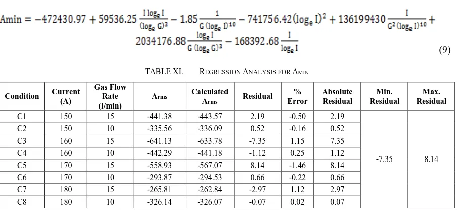
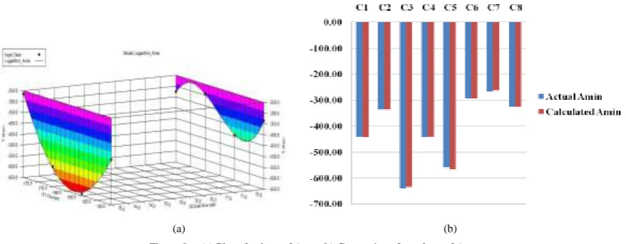
The regression model for Amin is as follows.

(9)

TABLE XI. REGRESSION ANALYSIS FOR AMIN

Condition Current (A)

Gas Flow Rate (l/min)

Arms Calculated

Arms Residual

% Error

Absolute Residual

Min. Residual

Max. Residual

C1 150 15 -441.38 -443.57 2.19 -0.50 2.19

-7.35 8.14

C2 150 10 -335.56 -336.09 0.52 -0.16 0.52

C3 160 15 -641.13 -633.78 -7.35 1.15 7.35

C4 160 10 -442.29 -441.18 -1.12 0.25 1.12

C5 170 15 -558.93 -567.07 8.14 -1.46 8.14

C6 170 10 -293.87 -294.53 0.66 -0.22 0.66

C7 180 15 -265.81 -262.84 -2.97 1.12 2.97

(a) (b)

Figure 8. (a) Plot of values of Amin (b) Comparison for values of Amin

As all the values obtained are less than zero, the plot is in inverted manner. Also, negligible difference between calculated and generated values of Amin is found, which indicates accuracy of the designed model.

C. Regression for Arms

TABLE XII. VALUES OF ARMS FOR EACH PASS

The regression model for Arms is as follows.

(10)

TABLE XIII. REGRESSION ANALYSIS FOR ARMS

Condition Current (A)

Gas Flow

Rate (l/min) Arms

Calculated

Arms Residual % Error

Absolute Residual

Min. Residual

Max. Residual

C1 150 15 30.72 30.57 0.14 0.47 0.14

- 0.49 0.54

C2 150 10 31.12 31.09 0.03 0.11 0.03

C3 160 15 31.12 63.22 -0.49 -0.78 0.49

C4 160 10 58.68 58.75 -0.07 -0.13 0.07

C5 170 15 63.67 63.14 0.54 0.85 0.54

C6 170 10 27.42 27.37 0.04 0.16 0.04

C7 180 15 27.71 27.90 -0.20 -0.71 0.20

C8 180 10 24.91 24.91 0.00 -0.02 0.00

Values of Arms for each pass

Arms1 Arms2 Arms3 Arms4 Arms5 Average Amax

37.13 24.95 22.80 28.24 40.47 30.72

40.80 35.24 21.12 34.42 24.02 31.12

89.35 55.82 54.40 49.21 64.87 62.73

65.29 63.11 55.08 58.27 51.64 58.68

69.70 89.35 55.81 54.40 49.11 63.67

20.20 31.69 26.49 29.91 28.80 27.42

27.95 28.18 28.32 22.24 31.84 27.71

(a) (b)

Figure 9. (a) Plot of values of Arms (b) Comparison for values of Arms

As all the values obtained are less than zero, the plot is in inverted manner. Also, almost all the calculated values match the generated values of Arms is found. Hence, the model indicates precision.

V. CONCLUSION

The mathematical models designed can predict intermediate sound pressure values which can be helpful in weld quality prediction and thereby result in improved weld. Characterization of the process can be developed by increasing numerical and experimental evaluations for GTAW process at different working environment so that accurate standardized system of online weld monitoring can be developed with diminished level of error. The combined effect of welding and locating induced defects can be considered for controlling the quality of weld. Also, once the cause of generation of defects is known, modifications can be made in the process parameters to achieve minimization of defects. Comparisons between numerical predictions and experimentally obtained values can be portrayed by graphical representations and surface plot.

REFERENCES

[1] Kaustubh Samvatsar, Rakesh Barot, Hardik Beravala, Vikas Chhillar, ― Feasibility Study for In-Process Monitoring of Gas Tungsten Arc Welding‖, International Journal of Engineering Research and Development, Vol. 11, Issue 4, pp.27-31, April 2015

[2] Hyeong-Soon Moon, Suck-Joo Na, ―Optimum Design Based on Mathematical Model and Neural Network to Predict Weld Parameters for Fillet Joints‖, Journal of Manufacturing Systems, Vol. 16, Issue 1, pp.13-23, 1997

[3] Na Lv, Yanling Xu, Zhifen Zhang, Jifeng Wang, Bo Chen, Shanben Chen, ―Audio sensing and modeling of arc dynamic characteristic during pulsed Al alloy GTAW process", Sensor Review,Vol. 33, Issue 2, pp.141 – 156, 2013

[4] Jožef Horvat, Jurij Prezelj, Ivan Polajnar, Mirko Čudina, ―Monitoring Gas Metal Arc Welding Process by Using Audible Sound Signal‖, Strojniški vestnik - Journal of Mechanical Engineering, Vol. 57, Issue 3, pp. 267-278, 2011

[5] S.P.Gadewar, Peravli Swaminadhan, M.G.Harkare, S.H.Gawande, ―Experimental investigation of weld characteristics for a single pass TIG welding with SS304‖, International Journal of Engineering Science and Technology, Vol. 2 Issue 8, pp. 3676-366, 2010 [6] R.Sathish, B.Naveen, P.Nijanthan, K.Arun Vasantha Geethan, Vaddi Seshagiri Rao, ―Weldability and Process Parameter Optimization

of Dissimilar Pipe Joints Using GTAW‖, International Journal of Engineering Research and Applications, Vol. 2, Issue 3, pp. 2525-2530, May-Jun 2012

[7] Fujii, H., Sato, T., Lu, S.P., Nogi, K., ―Development of an advanced A-TIG welding method by control of Marangoni convection‖, Material Science Engineering, Vol. 495, pp. 296–303, 2008

[8] Kaustubh Samvatsar, Rakesh Barot, Hardik Beravala, ―Design of Fixture for Evaporator Rotor Assembly‖, International Journal of Innovative Research in Science, Engineering and Technology, Vol. 4, Issue 6, pp. 4045-4052, June 2015, DOI:

10.15680/IJIRSET.2015.0406030.

[9] Jigar R. Patel, Kaustubh S. Samvatsar, Haresh P. Prajapati, Shyam S. Rangrej, ―Optimization of Process Parameters for Reducing Surface Roughness Produced During Single Point Incremental Forming Process‖, International Journal on Recent Technologies in Mechanical and Electrical Engineering, Vol. 2 Issue 9, pp. 019-023, Sept. 2015.

[10] Purvi Chauhan, Shyam Rangrej, Kaustubh Samvatsar, Jigar Patel, ―A Review on Scope, Study & Need of Setup Time Reduction for Conveyor Pulley Manufacturing‖, International Journal of Advance Research in Engineering, Science & Technology, Vol. 2, Issue 3, pp.29-33, March- 2015.

[11] Kaustubh S .Samvatsar, Rakesh S. Barot, Hardik S. Beravala, ―Product Development Procedure for Designing a Fixture‖, Proceedings of 6th National Conference on Emerging Vistas of Technology in 21st Century , April 2015, DOI: 10.13140/RG.2.1.2065.7124. [12] Purvi Chauhan, Shyam Rangrej, Kaustubh Samvatsar, Jigar Patel, ―Feasibility Study for Waste Reduction Using JIT Concept – A Case

of Forging Industry‖, Proceedings of 5th National Conference on ―Recent Advances in Manufacturing‖, May, 2015, DOI: 10.13140/RG.2.1.4032.8163.