A Spectral Element Method Formulation for
Rectangular thin Plates
Nivaldo Benedito Ferreira Campos1, José Maria Campos dos Santos2
1Department of Structural Engineering, School of Civil Engineering, Architecture and Urbanism, UNICAMP 2Department of Computational Mechanics, College of Mechanical Engineering, UNICAMP.
1[email protected], 2[email protected]
Abstract-- In the mid-frequency range, numerical methods such as the finite and boundary element methods are not the most suitable for structural dynamic analysis as mesh refinement leads to models that are often too large. Other methods that can be considered as semi-analytical, such as the spectral element method, do not need that at higher frequencies a mesh refinement be done, but they are limited in the geometries that can be modeled and some of its formulation cannot treat arbitrary boundary conditions. This work develops a spectral element for thin plates based on a high precision finite element proposed by Kulla, which can be applied on modeling plates with arbitrary boundary conditions. The results obtained are compared with others from different methods presented in the literature.
Index Term-- Spectral element method, plate, vibrations, numerical methods, frequency response functions.
1.INTRODUCTION
Nowadays, the most commonly used methods for dynamic simulations of mechanical structures are the Finite Element Method (FEM) (Zienkiewicz and Taylor [1]) and the Boundary Element Method (BEM) (Banerjee and Butterfield, [2]), which are deterministic methods. Both are based on the discretization of the structure into small elements, in which the dynamic field variables are expressed in terms of approximated shape functions. As a consequence of this characteristic, a structural analyses at medium and high frequencies performed using these techniques will require that as the frequency increases the size of the elements becomes smaller, while its number will increase. For structures that are common in many engineering areas, this will be only possible with a large amount of computational effort, restricting the use of such methods mostly to low-frequency applications.
For high-frequency modeling, probabilistic techniques such as the Statistical Energy Analysis (SEA) (Lyon and DeJong, [3]) have been developed. In this technique, the model is divided in a number of subdomains, for which only averaged energy levels are predicted. Therefore, it is unable to give results at discrete points of the problem domain. As any other method, its accuracy depends on the validity of the assumptions that were made, and in the case of SEA, these assumptions are high modal density and light coupling between subsystems in the frequency range of interest. Often, they are not valid in the middle frequency range or in
structures with stiff members connected to thin shells, which limits the use of the method to the high-frequency range.
For applications at mid-frequency range, adequate prediction techniques are still not available because the computational costs of conventional techniques based on elements are already too high, while the assumptions assumed by probabilistic techniques are not valid yet.
In an attempt to overcome these difficulties, it have recently been developed many attractive methodologies based on an indirect Trefftz approach (Jin et al., [4], Desmet et al., [5]), which can be classified as wave based methods. These methods do not require mesh discretization to model a domain with constant geometric and physical properties, since the pressure or displacement fields are described by wave functions that exactly satisfy the differential equation of the problem. The solutions, obtained as an infinite series truncated accordingly to the desired precision, are able to describe an infinite number of modes and are obtained by determining the unknown contribution of the wave factors, what is done by introducing the boundary conditions of the problem. The matrices produced are smaller than the ones from FEM and BEM, and in spite of the fact that they are fully populated and frequency dependent, it has proven that the methods are computationally more efficient for the analysis of steady-state vibroacoustic problems.
A comprehensive overview of the methodologies used in the wave based methods is presented by Desmet [6]. Among them, in the area of structural dynamics, it should be mentioned the superposition method, developed by Gorman [7], and applied mainly to model free-free plates. The image method, first used in modeling acoustic problems, was extended by Gunda et al. [8] to treat beams and plates. Kulla [9] presented a high precision finite element method, which was able to model beams and plates with arbitrary boundary conditions. The same approach was used by Kevorkian and Pascal [10] and Casemir et al. [11] on the continuous element method. Lee and Lee [12] applied the spectral element method to model Levy type plates and Doyle [13] gave a Fourier approach to it. Arruda et al. [14] extended the work of Lee and Doyle, developing a spectral element for reinforced panels.
1511202-4848-IJECS-IJENS © April 2015 IJENS I J E N S
cases. It is presented a technique based in the energy concept to introduce any kind of load distribution. In order to make the method readily understandable, its aspects that are not essential were omitted on the development of the formulation. Numerical examples were developed to demonstrate the accuracy of the method and the results were compared with those obtained with other methods.
2.SERIES SOLUTION FOR THE KIRCHHOFF PLATE EQUATION Let us consider a Kirchhoff plate subject to a transverse dynamic load. The governing equation of the forced transversal vibration w of this kind of plate can be expressed as
2 4
2
, ;
w
D
w
h
P x y t
t
(1)where
3 2
12 1
E h
D
(2)Considering just the case of steady-state bending vibration in which is acting a time harmonic force, it can be assumed that the force has the form P(x,y;t)=P(x,y) e i t. Accordingly, the transversal displacements will be expressed
as w(x,y,t)=w(x,y) e i t. Introducing these expressions into
eq. (1), it becomes
4 4 ,
f
P x y w k w
D
(3)
where 2 4 f
h
k
D
(4)In order to solve eq. (3), in its homogenous form
4 4
0
fw k w
(5)it will be assumed a solution of the form
( , ; )
p x q yw x y
C e
e
(6)for a rectangular plate with dimensions Lx = 2a and Ly=2b, and C constant.
Introducing eq. (6) into eq.(5), it will be obtained the characteristic equation or the homogeneous biharmonic differential equation as
2 2 2 4 2 2 2
(
p
q
)
k
f
0
or
p
q
k
f (7)There are infinite values of p and q that satisfy Eq. (7). Let us assume that the solution in the x direction can be expanded as an exponential Fourier series. A general term of this series for a given m, will be expressed as
,
0, 1, 2,
x m m
i m
x i k x
p x a
m m m
C e
C e
C e
m
(8)and, therefore
m x m
i m
p
i k
a
withk
xmm
a
(9)Introducing the expression for pm into eq. (7), it will define qm as
2 2
m x m f
q
k
k
(10)which can be rewritten as
2 2
1 1
2 2
2 2
m f x m y m
m f x m y m
q
i k
k
ik
q
k
k
k
(11)and, therefore, a given m will yield eight basis solutions for eq. (5), which grouped in a set can be expressed as
1 1 2 2
1 1 2 2
1 1 2 3 4
5 6 7 8
y m y m y m y m x m
y m y m y m y m x m
i k y i k y k y k y i k x
m m m m m
i k y i k y k y k y i k x
m m m m
w
C e
C e
C e
C e
e
C e
C e
C e
C e
e
(12)where
2 2 2 2
1 2
2 2 2 2
1 2
x n f y n x n f y n
y n f x n y n f x n
k
k
k
k
k
k
k
k
k
k
k
k
(13)Appling the same approach to the solution in the y
direction, q can be expressed as
n y n
q
i k
withk
ynn
b
(14)Introducing the expression for qm into eq. (7), it will define pm as
2 2
n y n f
p
k
k
(15)which can be rewritten as
2 2
1 1
2 2
2 2
n f y n x n
n f y m x n
p
i k
k
ik
p
k
k
k
1511202-4848-IJECS-IJENS © April 2015 IJENS
and, therefore, a given n will yield another eight basis solutions for eq. (5), which grouped in a set can be expressed as
1 1 2 2
1 1 2 2
2 1 2 3 4
5 6 7 8
x m x n x n x n y n
x n x n x n x n y n
i k x i k x k x k x i k y
n n n n n
i k x i k x k x k x i k y
n n n n
w
C e
C e
C e
C e
e
C e
C e
C e
C e
e
(17)The solution for the homogenous differential equation (5) will be therefore
1 2 1 2
0 0 0
( , ; )
m n n nm n n
w x y
w
w
w
w
(18)whose explicit form for a given n is
1 1 2 2
1 1 2 2
1 1 2 2
1 1 2
1 2 3 4
5 6 7 8
9 10 11 12
13 14 15
( , ; )
y n y n y n y n x ny n y n y n y n x n
x m x n x n x n y n
x n x n x n
i k y i k y k y k y i k x
n n n n n
i k y i k y k y k y i k x
n n n n
i k x i k x k x k x i k y
n n n n
i k x i k x k x
n n n
w x y
C e
C e
C e
C e
e
C e
C e
C e
C e
e
C e
C e
C e
C e
e
C e
C e
C e
2
16
x n y n
k x i k y n
C e
e
(19)
and the general expression for the displacement, in matrix form is
( , ; )
w x y
Ψ c
T
(20) where is a vector of basis functions and c a vector of integration constants.
As pointed out by Casimir et al. (2005), this solution is valid within the theoretical limits required by Kirchhoff theory. This means that the ratio between the thickness of the plate and the wavelength should be far less than unity, which will restrict the frequency range of validity of eq. (19). Assuming a ratio less than 0.1, it can be shown that the frequency limit is
2 2
0.04
D
h
h
(21)3.SPECTRAL DYNAMIC STIFFNESS MATRIX
In order to develop an elemental spectral stiffness matrix for thin plates, the trigonometric form of eq. (19), split into its four cases of symmetry, was used.
( , ; )
n( , ; )
nSS( , ; )
nSA( , ; )
nAS( , ; )
nAAw x y
w x y
w x y
w x y
w x y
(22)and
1 1 2 2
3 1 4 2
( , ; )
cos
cos
cosh
cos
cos
cosh
SS
n x n n y n n y n
y n n x n n x n
w x y
k x C
k
y
C
k
y
k y C
k
x
C
k
x
(23)
5 1 6 2
7 1 8 2
( , ; )
cos
sin
sinh
sin
cos
cosh
SA
n x n n y n n y n
y n n x n n x n
w x y
k x C
k
y
C
k
y
k y C
k
x
C
k
x
(24)
9 1 10 2
11 1 12 2
( , ; )
sin
cos
cosh
cos
sin
sinh
AS
n x n n y n n y n
y n n x n n x n
w x y
k x C
k
y
C
k
y
k y C
k
x
C
k
x
(25)
13 1 14 2
15 1 16 2
( , ; )
sin
sin
sinh
sin
sin
sinh
AA
n x n n y n n y n
y n n x n n x n
w x y
k x C
k
y
C
k
y
k y C
k
x
C
k
x
(26)where for sine functions
2 1
2 xn n k a
,
2 1
2 yn n k b
n = 0.1, 2,.. (27)
and for cosine functions
xn
n
k
a
,k
ynn
b
n = 0, 1, 2, … (28)The thin plate spectral dynamic stiffness matrix can be obtained by writing the shear forces V and the moments M as a function of the displacements and slopes at the boundaries along the x and y directions. These terms are defined by the well known relations
( , ; )
, ;
xw x y
x y
x
(29)
( , ; ) , ; yw x y x y
y
(30)
2 2 2 2( , ; )
( , ; )
M
xx y
, ;
D
w x y
w x y
x
y
(31)
2 2 2 2( , ; )
( , ; )
, ;
yw x y
w x y
M
x y
D
y
x
(32)
3 3
3 2( , ; )
( , ; )
V
xx y
, ;
D
w x y
2
w x y
x
x y
(33)
3 3
3 2( , ; )
( , ; )
, ;
2
y
w x y
w x y
V x y
D
y
x y
1511202-4848-IJECS-IJENS © April 2015 IJENS I J E N S
Evaluating eq. (22), (29) and (30) at the boundaries and assembling the results, a vector d of displacements on the boundaries, is obtained
.
d
D c
(35)where
( , ) {
,
,
,
,
,
,
,
, }
Tx x y y
x y
w
a y w a y
w x b
w x b
a y
a y
x b
x b
d
(36)
1 1 1 1 1 1
1,0 16,0 1,1 16,1 1, 16,
2 2 2 2 2 2
1,0 16,0 1,1 16,1 1, 16,
8 8 8 8 8 8
8 16 1,0 16,0 1,1 16,1 1, 16,
( , )
n n
n n
x n
n n
d
d
d
d
d
d
d
d
d
d
d
d
x y
d
d
d
d
d
d
D
(37)
1
16,n sinh 2x n( ) sin y n
d k a k y (38)
1,0 16,0 1,1 16,1 1, 16,
T
n n
C C C C C C
c (39)
Proceeding in the same way in relation to the forces at the boundaries, it will be obtained
f
F c
(40)where
{-v
,
v
,
-v
,
v
,
-m
x,
m
x,
-m
y,
m
y, }
Ta y
a y
x b
x b
a y
a y
x b
x b
f
(41)
1 1 1 1 1 1
1,0 16,0 1,1 16,1 1, 16,
2 2 2 2 2 2
1,0 16,0 1,1 16,1 1, 16,
8 8 8 8 8 8
8 16 1,0 16,0 1,1 16,1 1, 16,
n n
n n
x n
n n
f
f
f
f
f
f
f
f
f
f
f
f
f
f
f
f
f
f
F
(42)
1 2 2
16,n 2x n y n 2 2x n cosh 2x n( ) sin y n
f k k
k k a k y (43) In order to eliminate the dependence on x and y of , ,d D f and F , they will be expanded in a trigonometric Fourier series and the coefficients of the sine and cosine terms will be placed in two different lines. Truncating this series at an adequate number of terms m, the resulting constant matrices will be square. In this way, we will have
1
f
F c
T f
T F c
f
F c
c
F
f
(44)
1
d D c
T d T D c
d D c
c
D
d
(45)where 0 1 2 n
T
T
T
T
T
(46) where
cos 0 0 0
2 1
0 sin 0 0
2
0 0 cos 0
2 1
0 0 0 sin
2 xn n x a n x a n x a n x a
T (47)
cos 0 0 0
2 1
0 sin 0 0
2
0 0 cos 0
2
2 1
0 0 0 sin
2 yn n y b n y b n y b n y b
T (48)
Eliminating c from eq. (44) and (45), it yields
S d f
(49)where S, the dynamic stiffness matrix, is given by 1
S
F D
(50)For plates with free-free or clamped-clamped boundary conditions, its natural frequencies and modes can be obtained by setting respectively the vectors f or d equal to zero on eq. (49) and solving the resulting eigenproblem.
4.SOLUTION OF THE FORCED CASE
1511202-4848-IJECS-IJENS © April 2015 IJENS
,
a b
a b
W
P x y wdx dy
d
T
f
d
(51)If the forces are applied only at the boundary, w can still be obtained with the homogeneous formulation by using eq. (20) and (45) , as
1
( , ; )
w x y
Ψ D
T
d
(52) which introduced in eq. (51), results in
1¨
,
a b
a b
P x y
dx dy
d
Ψ D
Td
f
TT T d
T(53) or
1 2¨
,
a b
a b
P x y
dx dy
d
Ψ
TD
d f
T
T
d
(54) Adopting
¨
,
a b
a b
P x y
dx dy
p
c
Ψ
(55)
1 2d
po
pn p
pn
T
0
0
0
0
T
0
0
T
T
0
0
T
0
0
0
0
(56)
with
16 16
1
0
0
0
0
0
0
0
...
1
0
0
0
0
0
0
0
...
1
0
0
0
0
0
0
0
...
1
0
0
0
0
0
0
0
...
1
0
0
0
0
0
0
0
...
1
0
0
0
0
0
0
0
...
1
0
0
0
0
0
0
0
...
1
0
0
0
0
0
0
0
...
:
:
:
:
:
:
:
:
xb
b
b
b
a
a
a
a
pn
T
(57),
8 8
1
0
0
0
...
2
1
0
0
0
...
2
1
0
0
0
...
2
1
0
0
0
...
2
:
:
:
:
xb
b
a
a
po
T
(58)it leads to determine f as T
p
pf
T D
c
(59)Using the value of f provided by eq. (59) and introducing the boundary conditions on eq. (49), in the same way as it is done in the finite element method, one obtain the value of d which introduced in equation (52) will completely determine the displacement field. In order to obtain a more general formulation, suitable to treat the case of general loading applied to the domain, the general solution of eq. (1) should be used in generating eq. (35) and (40), but as it will be shown in the second numerical example, the use of the approach presented in this section can give accurate results for the natural frequencies, even when the loads are applied in the domain, provided that the points of application are near the boundary.
5.NUMERICAL EXAMPLES
In this section it is presented numerical implementations of the SEM to validate its formulation. Similar examples can be found in the works of Lee and Lee [12], Casimir et al. (2005), and Kevorkian and Pascal (2001), but in these works different settings of basis functions are used to model each boundary condition. Here, it is shown that a unique formulation can be used to model any boundary condition.
5.1.LEVY TYPE PLATE
1511202-4848-IJCEE-IJENS © April 2015 IJENS I J E N S Fig. 1. FRFs obtained with SEM formulated in this work and with a spectral formulation for Levy type plates.
A unitary harmonic concentrated load is applied at the mid span of a free edge and the frequency response functions obtained were compared in the interval between 0 e 1000 Hz, as shown in Fig. 1. Both methods used five terms of the expansion in Fourier series. The agreement between then is nearly perfect.
The plate modeled has the following properties: 0.5 x 0.5 m, = 2800 kg/m3, h = 0.001 m, = 0.3, = 0.003, E = 73.5 Mpa.
5.2.SIMPLY SUPPORTED PLATE
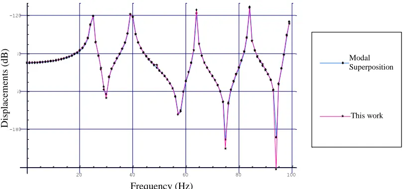
To verify the accuracy of the method, a simply supported plate was modeled with SEM and the resulting FRFs were compared with those from a solution obtained by
modal superposition. The excitation with a unitary harmonic punctual load was done at (x=0.49, y=0.24) and the response point taken at (x=0.2, y=0.1). The modal superposition solution was obtained taking into account 400 modes and the SEM solution was obtained taking 5 terms of the Fourier series. The plate modeled has the following properties: Lx = 1.0, Ly = 0.5 m, = 7800 kg/m3, h = 0.002 m, = 0.3, E = 210 MPa. Even considering the fact that the load was applied in the domain (but near the boundary), a good agreement was achieved (Fig. 2).
Fig. 2. FRFs obtained with SEM and with a modal superposition solution. 5.3.FREE PLATE
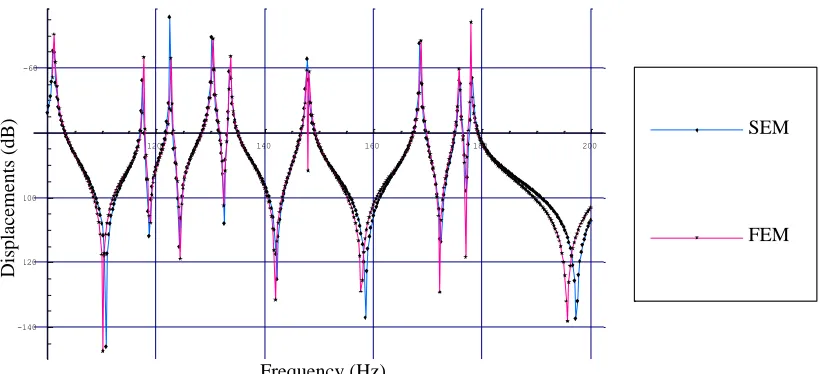
The same model of SEM used in the previous example, with five terms of the Fourier series expansion, but with a free-free-free-free boundary condition, is now compared with
a FEM model of 1050 four-node quadrilateral elements (Przemieniecki [15]. A Guyan reduction was used to compute a reduced number of normal modes, but the residual flexibility of the truncated modes was taken into account. The unitary
200 400 600 800 1000
-160 -140 -120 -100
Kulla Arruda
20 40 60 80 100
-180 -160 -140 -120
SEM Modal
Lee
This work
Frequency (Hz)
Dis
p
lace
m
en
ts
(
d
B
)
Modal Superposition
Frequency (Hz)
Dis
p
lace
m
en
ts
(
d
B
)
1511202-4848-IJECS-IJENS © April 2015 IJENS
load is applied at a corner and its response is measured at the same position. The results are in good agreement (fig. 3) in all the plotted frequency range, except in the region where the last antiresonance appears. This is due to the fact that, at higher frequencies, the effect of modal truncation becomes
more relevant in the FE model. Considering the number of finite elements needed to achieve this accuracy, the use of SEM, although it yields a fully populated stiffness matrix, is fully justified.
Fig. 3. FRFs obtained with SEM and FEM 6.FINAL REMARKS
It was developed a spectral element for thin plates which can be used to model plates with any kind of boundary conditions and a detailed description on how to obtain all the terms needed to implement it was presented. The results obtained using this element proved to be appealing and its accuracy (comparable to the accuracy obtained with modal superposition) makes it a potential tool for structural analysis of thin plates in mid and high frequency ranges. Further development of this method to allow the application of any kind of loads in the domain and the modeling of domains with polygonal shapes should be carried out in order to make it possible to use this method to analysis structures with shapes other than rectangular.
REFERENCES
[1] Zienkiewicz, O.C. and Taylor, R.L., 2000, “The Finite Element Method – Volume 1: the basis”, Fifth Edition, Butterworth-Heinemann, Boston. [2] Banerjee, P.K. and Butterfield, R., 1981, “Boundary Element Methods
in Engineering Science”, McGraw-Hill Book Company, UK.
[3] Lyon, R.H. and DeJong, R.G., 1995, “Theory and Application of Statistical Energy Analysis”, Butterworth-Heinemann, Boston. [4] Jin, W.G., Cheung, Y.K. and Zienkiewicz, O.C., 1993, ”Trefftz method
for Kirchhoff plate bending problems”, International Journal for Numerical Methods in Engineering 36, 765-781.
[5] Desmet, W., Sas, P. and Vandepitte, D., 2001, “An indirect Trefftz-method for the steady-state dynamic analysis of coupled vibro-acoustic systems”, Computer Assisted Mechanics and Engineering Sciences, 8, 271-288
[6] Desmet, W., 2002, “Mid-frequency vibro-acoustic modelling: challenges and potential solutions”, in Proceedings of ISMA2002 - Volume II, Leuven, Belgium, pp. 835-862.
[7] Gorman, D. J., 1999, “Vibration Analysis of Plates by the Superposition Method” (Series on Stability, Vibration and Control of Systems Series a, Volume 3), World Scientific Publishing Company, 270 p.
[8] Gunda, R., Vijayakar, S.M. and Singh, R., 1995, “Method of images for the harmonic response of beams and rectangular plates”, Journal of Sound and Vibration 185(5), pp. 791-808.
[9] Kulla, P.H., 1997, “High precision finite elements”, Finite Elements in Analysis and Design 26, pp. 97-114.
[10] Kevorkian, S. and Pascal, M., 2001, “An accurate method for free vibration analysis of structures with application to plates”, Journal of Sound and Vibration 246 (5), pp. 795–814.
[11] Casimir, J.B., Kevorkian, S. and Vinh, T., 2005, “The dynamic stiffness matrix of two-dimensional elements: application to Kirchhoff’s plate continuous elements”, Journal of Sound and Vibration 287, pp. 571–589
[12] Lee, U. and Lee, J., 1999, “Spectral-element method of Levy-type plates subjected to dynamic loads”, Journal of Engineering Mechanics, February, pp. 243-247.
[13] Doyle, J.F., 1997, “Wave propagation in structures: spectral analysis using fast discrete Fourier transforms”, 2nd ed., Springer-Verlag. [14] Arruda, J.R.F., Donadon, L.V., Nunes, R.F. and Albuquerque, E.L.,
2004, “On the Modelling of Reinforced Plates in the mid-frequency range”, INTERNOISE 2004 - The 13th International Congress and Exposition on Noise Control Engineering, Prague, Czech Republic, August 22-25.
[15] Przemieniecki, J.S., 1985, “Theory of matrix structural analysis”, Dover, New York.
120 140 160 180 200
-140 -120 -100 -60
FEM SEM
SEM
FEM
Frequency (Hz)
Dis
p
lace
m
en
ts
(
d
B