Interest Rate And Stock Market
Returns In Namibia
Joel Hinaunye Eita, North-West University, South Africa
ABSTRACT
This paper analyses the causal relationship between interest rate and stock market return in Namibia for the period 1996 to 2012. The analysis was done through cointegrated vector autoregression methods. The analysis reveals that there is a negative relationship between stock market returns and interest rates in Namibia. Causality test indicates that there is bi-directional causality between stock market returns and interest rate in Namibia. The results suggest that contractionary monetary policy through higher interest rate decreases stock market returns in Namibia.
Keywords: Interest Rates; Stock Market Returns; Causality; Cointegration
1. INTRODUCTION
he response of asset prices to interest rate policy is a key component for investigating the impact of monetary policy economy. Interest rate policy has important effects on the economy because it moves financial market prices that matter, such as stock market values. The stock market is one sector of the economy that is affected by changes in interest rate and stock prices change in response to interest rate. Hence, the relationship between interest rate and the price of assets is important to policymakers.
In Namibia, growth in the activities of the stock market and increase in the listing of companies on the Namibian Stock Exchange have implications on the economy. The interest policy is an important tool in addressing macroeconomic policy in Namibia. Changes in interest rate can have a significant influence on the returns of the stock market. As Adjasi and Biekpe (2006) noted, stock prices can also influence movements in interest rate. Investors and analysts can react more to comments of Governors of central banks on the direction of interest rate. Rigobon and Sack (2001) argue that monetary policy reacts significantly to movements in stock markets, which raises an important question on whether central banks should conduct interest rate policies in response to movements in the price of stocks or whether they should also react to movements in the prices of stocks.
Despite the fact that the relationship between interest rate and stock market returns is important for policy, empirical studies on this relationship are limited. The objective of this paper is to present a test of the causal relationship between interest rate and stock market returns in Namibia.
The paper is organised as follows: Section 2 presents the literature review; Section 3 presents the empirical model and the Granger causality procedure; Section 4 outlines the econometric technique and methodology; results are presented in Section 5; and Section 6 concludes.
2. LITERATURE REVIEW
Literature on the relationship between interest rate and stock market is not without ambiguity. The issue of whether interest rates should be responsive to movements in the prices of the stock market depends on the empirical evidence and the economic environment (Adjasi & Biekpe, 2006). Whether monetary policy, through interest rate, affects stock market returns is still an open question.
Mishkin (1995) states that interest rate changes are a transmission mechanism through which monetary policy affects the prices of assets. When the supply of money declines, individuals and companies will find that they have less money than they want and then reduce their spending. The stock market is one place where they can spend less money, decreasing the demand for stocks, which in turn depresses their prices. According to Mishkin (1995) a rise in interest rate resulting from contractionary monetary policy makes bonds more attractive compared to equities and this causes the price of equities to decrease. This results in a decline in investment spending as well as lower output. Thorbecke (1997) provides evidence that expansionary monetary policy (reducing interest rate) causes a rise in stock market returns. Interest rate policy has important effects on real variables. Smal and de Jager (1997) argue that reduction in interest rate results in more liquidity into the economy. The extra liquidity is taken to the stock market which causes a rise in the demand and prices of stock. Ehrmann and Fratzscher (2004) investigate the effect of monetary policy on stock returns and find that stock market returns react negatively to interest rates. These studies provide evidence that stock market returns react negatively to increases in interest rate.
There are studies which conclude that changes in interest rates may not be enough to influence changes in stock market prices or returns. Bernanke and Gertler (1999, 2001) showed that because asset prices are volatile, it is not easy to predict and interest rates should only be changed in reaction to movements in stock prices when it is expected that such movements will affect inflation. Bernanke and Gertler argue that if interest rates change in response to movements in the price of assets, the credibility of the interest rate policy will be reduced. Bernanke and Kuttner (2003) also showed that changes in interest rates do not have a significant impact on stock market returns. Davig and Gerlach (2006) supported this view that the relationship between the prices of stocks and interest rates changes is not significant.
Other studies argue that interest rates should respond to changes in the prices of stocks because misalignment in stock prices can impact negatively on the economy. Bordo and Jeanne (2001) argued that a sharp increase in stock prices causes inflation and, on the other hand, a sharp decrease in stock prices can cause a decline in the economic activity. Rigobon and Sack (2003) state that the stock market has a significant impact on the economy and is an important variable in the determination of monetary policy. Monetary policy responds significantly to changes in stock market returns. Adjasi and Biekpe (2006) found that there is a long-run relationship between interest rates and stock market returns in Kenya and South Africa. This relationship was positive for Kenya but negative for South Africa. The literature does not provide a clear direction on the relationship between interest rate and stock market returns which means that the causal relationship between interest rate and stock market returns remains an open question or an empirical issue.
3. EMPIRICAL MODEL: GRANGER CAUSALITY THEORY
The empirical model applied in this study is based on one used by Ehrmann and Fratzscher (2004) and Bernanke and Kuttner (2005), which is specified as follows:
t t t a bI e
SMR (1)
whereSMRt, It, and et are stock market returns, interest rate, and error term.
Granger causality test is applied to Equation (1) to test the causal relationship between interest rate and stock market returns. The test was developed by Granger (1969) and states that a variable (in this case interest rate) is said to Granger cause another variable (stock market returns) if past and present values of interest rate help to predict stock market returns. A third variable is added to Equation (1) to avoid the problem of omitted variable bias. The omitted variable bias normally happens when causality is tested using only two variables in the equation. For that reason, the exchange rate was added to Equation (1) in order to avoid the problem of omitted variable bias. A Granger causality test involving three variables - stock market returns, interest rates, and exchange rate - is written as:
t p
j
j t j j
t p
j j p
j
j t j
t
SMR
I
ER
u
SMR
1 1
1
t p j j t j p j j t j p j j t j
t
SMR
I
ER
v
I
1 1 1
(3) t j t p j j p j j t j j t p j jt
SMR
I
ER
ER
1 1 1 (4)The null hypotheses to be tested are:
p
j
H
1:
j
0
,
1
...
states that interest rate does not Granger cause stock market returns.p
j
H
2:
j
0
,
1
...
states that exchange rate does not Granger cause stock market returns.p
j
H
3:
j
0
,
1
...
states that stock market return does not Granger cause interest rate.p
j
H
4:
j
0
,
1
...
states that exchange rate does not Granger cause interest rate.p
j
H
5:
j
0
,
1
...
states that stock market returns does not Granger cause exchange rate.p
j
H
6:
j
0
,
1
...
states that interest rate does not Granger cause exchange rate.Rejection of the hypotheses suggests that there is causality between variables. For example, if the first hypothesis is rejected, it shows that interest rate Granger causes stock market return. Rejection of the third hypothesis means that the causality runs from stock market returns to interest rate. If none of the hypotheses are rejected, it means that stock market return does not Granger cause interest rate and interest rate also does not Granger cause stock market return. It also means that there is no causality between exchange rate and stock market returns as well as interest rate. It indicates that the three variables are independent of each other. If all hypotheses are rejected, there is bi-directional causality between stock market returns, interest rates, and exchange rate.
The traditional Granger causality test uses the simple F-test statistic. Several studies, such as Chow (1987), Marin (1992), Pomponio (1996), McCarville and Nnadozie (1995), and Darat (1996), have used the traditional F-test to test for causality. The use of a simple traditional Granger causality has been identified by several studies (such as Engle & Granger, 1987; Toda & Yamamoto, 1995; Zapata & Rambaldi, 1997; Tsen, 2006) as not sufficient if variables are I(1) and cointegrated. If time series included in the analysis are I(1) and cointegrated, the traditional Granger causality test should not be used, and proper statistical inference can be obtained by analysing the causality relationship on the basis of the error correction model (ECM). Many economic time-series are I(1) and when they are cointegrated, the simple F-test statistic does not have a standard distribution. If the variables are I(1) and cointegrated, Granger causality should be done in the ECM and expressed as:
t p j t j t j j t p j j p j j t j
t
SMR
I
ER
u
SMR
1 1 1 1 1 1
(5) t p j t j t j p j j t j p j j t jt
SMR
I
ER
v
I
1 1 1 2 1 1
(6) t t j t p j j p j j t j j t p j jt
SMR
I
ER
ER
3 1 11 1
1
(7)
where
1t1,
2t1, and
3t2 are the lagged values of the error term from the cointegration estimations in4. ECONOMETRIC TECHNIQUE AND EMPIRICAL METHODOLOGY
The unit root test, which shows whether the variables are stationary or non-stationary, is the first step before estimation. The Augmented Dickey-Fuller (ADF) statistic is the most common used test for unit root, but it has limitations in the sense that it has low power. This study uses the Kwiatkowski, Phillips, Schmidt, and Shin (KPSS) in addition to ADF to test the stationarity or non-stationarity of the variables and their order of integration. If the variables are I(1), the next step is to test whether they are cointegrated. This is done by using the Johansen (1988, 1995) full information maximum likelihood. This econometric methodology corrects for autocorrelation and endogeneity parametrically using a vector error correction mechanism (VECM) specification. The detailed description of the Johansen procedure can be found in Johansen (1988), Johansen (1995), and Harris (1995).
5. DATA AND ESTIMATION RESULTS
5.1 Data
The study uses monthly data for the period 1996-2012. The data for Namibian Stock Exchange’s overall index (proxy for stock market returns) or lnSMR were obtained from the Namibian Stock Exchange. Exchange rate is defined as Namibia dollar per USA dollar (lnER), and interest rate is proxied by treasury bills rate (I). The data for exchange rate and interest rates were obtained from the Bank of Namibia.
5.2 Estimation Results
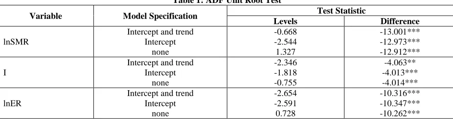
5.2.1 Unit Root Test
The ADF unit root test results are presented in Table 1 and the KPSS results are presented in Table 2.
Table 1: ADF Unit Root Test
Variable Model Specification Test Statistic
Levels Difference
lnSMR
Intercept and trend Intercept
none
-0.668 -2.544 1.327
-13.001*** -12.973*** -12.912***
I
Intercept and trend Intercept
none
-2.346 -1.818 -0.755
-4.063** -4.013*** -4.014***
lnER
Intercept and trend Intercept
none
-2.654 -2.591 0.728
-10.316*** -10.347*** -10.262***
Notes: */**/***/ significant or rejection of null of unit root at 10%/5%/1% significance level.
Table 2: KPSS Unit Root Test
Variable Model Specification Test Statistic
Levels Difference
lnSMR Intercept and trend
Intercept
1.633# 0.151#
0.057a 0.049 a
I Intercept and trend
Intercept
1.365# 0.186#
0.039 a 0.040 a
lnER Intercept and trend
Intercept
0.685# 0.211#
0.195 a 0.088 a
a indicates failure to reject the null hypothesis of stationarity at 5%. # indicates rejection of the null hypothesis of stationarity at 5%.
5.2.2 Cointegration Test, Long-Run and Granger Causality Test Results
Since the variables are nonstationary in levels, the appropriate modelling methodology is to the test for cointegration using the vector error correction model (VECM). The cointegration test results are presented in Table 3.
Table 3: Cointegration Test Results
Null Hypothesis Alternative Hypothesis Test Statistic 0.05 Critical Value Probability Valueb
Trace Statistic
r=0 r=1 30.811a 29.797 0.038
r=1 r=2 7.106 15.494 0.565
r=2 r=3 1.646 3.841 0.199
Maximum Eigenvalue Statistic
r=0 r>0 23.707 a 21.131 0.021
r≤1 r>1 5.460 14.264 0.683
r≤2 r>2 1.646 3.841 0.199
a denotes rejection of the null hypothesis at 0.05 level. b MacKinnon-Haug-Michelis (1999) p-values.
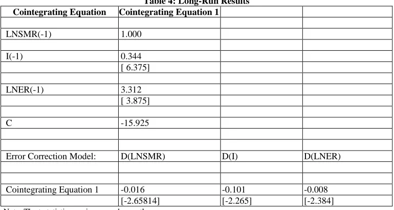
Table 3 indicates that there is one cointegrating vector. The lag length was set at 3 and was based on the Akaike information criterion, log likelihood ratio, final prediction error, Schwartz information criteria, and Hannan-Quinn information criterion. The diagnostic tests are performed on the VAR for stability, serial correlation, heteroscedasticity, and normality. The results indicate that they passed all diagnostic statistics. The VAR is stable, no serial correlation, no heteroscedasticity, and the residuals are multivariate normal. The diagnostic statistics are not presented here but are obtainable from the author upon request. The long run results are presented in Table 4 and those of Granger causality test are in Table 5.
Table 4: Long-Run Results
Cointegrating Equation Cointegrating Equation 1
LNSMR(-1) 1.000
I(-1) 0.344
[ 6.375]
LNER(-1) 3.312
[ 3.875]
C -15.925
Error Correction Model: D(LNSMR) D(I) D(LNER)
Cointegrating Equation 1 -0.016 -0.101 -0.008
[-2.65814] [-2.265] [-2.384]
Note: The t-statistics are in squared parentheses
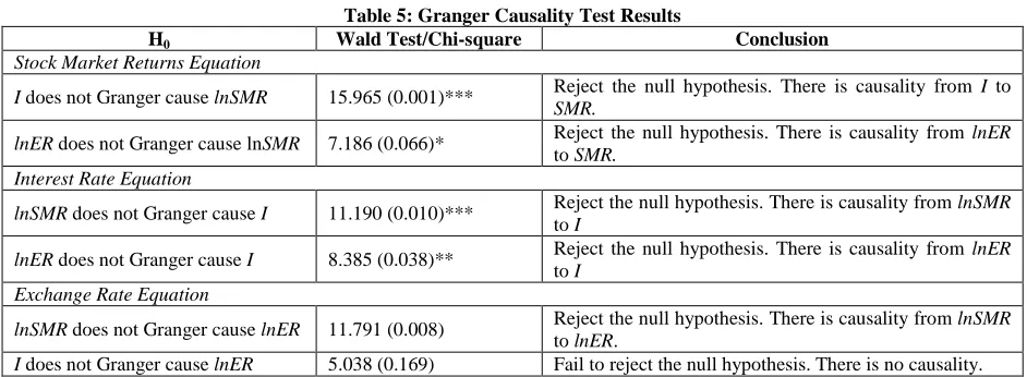
Table 5: Granger Causality Test Results
H0 Wald Test/Chi-square Conclusion
Stock Market Returns Equation
I does not Granger cause lnSMR 15.965 (0.001)*** Reject the null hypothesis. There is causality from I to
SMR.
lnER does not Granger cause lnSMR 7.186 (0.066)* Reject the null hypothesis. There is causality from lnER to SMR.
Interest Rate Equation
lnSMR does not Granger cause I 11.190 (0.010)*** Reject the null hypothesis. There is causality from lnSMR
to I
lnER does not Granger cause I 8.385 (0.038)** Reject the null hypothesis. There is causality from lnER to I
Exchange Rate Equation
lnSMR does not Granger cause lnER 11.791 (0.008) Reject the null hypothesis. There is causality from lnSMR
to lnER.
I does not Granger cause lnER 5.038 (0.169) Fail to reject the null hypothesis. There is no causality.
*/**/*** rejection of the null hypothesis of no Granger causality at 10/5/1 significance percent level. Note: Probabilities are in parentheses.
The Granger causality test results in Table 5 show evidence of causality from both directions. There is bi-directional causality between stock market returns and interest rates in Namibia and there is also bi-bi-directional causality between stock market returns and exchange rate. These are comparable to those obtained by Adjasi and Biekpe (2006) for South Africa.
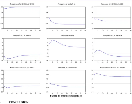
5.2.3 Impulse Responses
Impulse responses are introduced by Sims (1980) and show the response of one variable to shocks in another variable (for example, response of stock market returns to shocks in interest rate). They are important in the analysis of an estimated structural VAR. They show the dynamic response of a variable to a shock in one of the structural equations. They indicate the response of present and future values of each of the variables to a one-unit increase in the present value of one of the shocks of VAR. The impulse responses are presented in Figure 1. They are orthogononalised using Cholesky or lower triangular decomposition. The variables are ordered as stock market returns followed by interest rate and exchange rate.
-.08 -.04 .00 .04 .08
5 10 15 20 25 30 35 40
Response of LnSMR to LnSMR
-.08 -.04 .00 .04 .08
5 10 15 20 25 30 35 40
Response of LnSMR to I
-.08 -.04 .00 .04 .08
5 10 15 20 25 30 35 40
Response of lnSMR to lnEXCH
-.4 -.2 .0 .2 .4 .6 .8
5 10 15 20 25 30 35 40
Response of I to lnSMR
-.4 -.2 .0 .2 .4 .6 .8
5 10 15 20 25 30 35 40
Response of I to I
-.4 -.2 .0 .2 .4 .6 .8
5 10 15 20 25 30 35 40
Response of l to lnEXCH
-.04 -.02 .00 .02 .04 .06
5 10 15 20 25 30 35 40
Response of lnEXCH to lnSMR
-.04 -.02 .00 .02 .04 .06
5 10 15 20 25 30 35 40
Response of lnEXCH to I
-.04 -.02 .00 .02 .04 .06
5 10 15 20 25 30 35 40
Response of lnEXCH to lnEXCH
Figure 1: Impulse Responses
6. CONCLUSION
This paper analyses the causal relationship between stock market returns and interest rates in Namibia. The analysis was done through cointegrated vector autoregression and used monthly data covering the period 1996-2012. The results reveal that there is a negative relationship between interest rate and stock market returns in Namibia, which suggests that contractionary monetary policy through increase in interest rate reduces the stock market returns. A causality test indicates that there is bi-directional causality between stock market returns and interest rates, and the impulse responses show that they have long-lasting effect.
AUTHOR INFORMATION
Joel Hinaunye Eita, PhD, is a Professor of Economics at North-West University (South Africa). His research interests include international trade and finance, financial and monetary economics, time series econometrics, macro-econometric modelling, and panel data econometrics. He published in local and international journals. E-mail: hinaunye.eita@nwu.ac.za or hinaeita@yahoo.co.uk
REFERENCES
1. Adjasi, C. K. D., & Biekpe, N. (2006). Interest rate and stock market returns in Africa. African Finance
Journal, 8(2), 12-27.
2. Bernanke, B. S., & Gertler, M. (1999). Monetary policy and asset price volatility. Federal Reserve Bank of
Kansas City Economic Review, 84, 17-50.
3. Bernanke, B. S., & Gertler, M. (2001). Should central banks respond to movements in asset prices?
4. Bernanke, B. S., & Kuttner, K. (2005). What explains the stock market’s reaction to federal policy? Journal
of Finance, LX(3), 1221-1256.
5. Bordo, M., & Jeanne, O. (2001). Asset prices, reversals, economic and monetary. Paper Presented at the
Allied Social Science Association Meetings, New Orleans L.A.
6. Chow, P. C. Y. (1987). Causality between export growth and industrial development: Empirical evidence from the NICs. Journal of Development Economics, 26(1), 5-63.
7. Darat, A. F. (1996). Trade and development: The Asian experience. Cato Journal, 6(2), 695-699. 8. Davig, T., & Gerlasch, J. R. (2006). State-dependent stock market reactions to monetary policy.
International Journal of Central Banking, 2(4), 65-83.
9. Ehrmann, M., & Fratzscher, M. (2004). Taking stock: Monetary policy transmission to equity markets.
Journal Money, Credit and Banking, 36(4), 719-737.
10. Engle, R. F., & Granger, C. W. J. (1987). Co-integration and error correction: Representation, estimation and testing. Econometrica, 55(2), 251-276.
11. Granger, C. W. J. (1969). Investigating the causal relations by econometric models and cross-spectral methods. Econometrica, 37(3), 424-238.
12. Granger, C. W. J. (1988). Some recent developments in a concept of causality. Journal of Econometrics, 39, 199-211.
13. Harris, R. I. D. (1995). Using cointegration analysis in econometric modelling. London: Prentice Hall/Harvester Wheatsheaf.
14. Johansen, S. (1988). Statistical analysis of cointegrating vectors. Journal of Economic Dynamic and
Control, 12, 231-254.
15. Johansen, S. (1995): Likelihood based inferences in cointegrated vector autoregressive models, Oxford: Oxford University Press.
16. Marin, D. (1992). Is the export-led growth hypothesis valid for industrialised countries? Review of
Economics and Statistics, 74(4), 678-688.
17. Mishkin, F. S. (1995). Symposium on the monetary transmission mechanism. Journal of Economic
Perspectives, 9(4), 3-10.
18. McCarville, M., & Nnadozie, E. (1995). Causality test of export-led growth: The case of Mexico. Atlantic
Economic Journal, 23(2), 140-145.
19. Mohapi, P. L., & Motelle, S. I. (2007). Finance-growth nexus in Lesotho: Causality revelations from alternative proxies. Journal for Studies in Economics and Econometrics, 31(3), 43-59.
20. Pomponio, X. Z. (1996). A causality analysis of growth and export performance. Atlantic Economic
Journal, 24(2), 168-176.
21. Rigobon, R., & Sack, B. (2001). Measuring the reaction of monetary policy to the stock market. (NBER Working Paper Series, Working Paper 8350).
22. Smal, M. M., & de Jager, S. (2001). The monetary transmission mechanism in South Africa. (South African Reserve BankOccasional Paper No. 16).
23. Toda, H. Y., & Yamamoto, T. (1995). Statistical inference in vector autoregressions with possibly integrated processes. Journal of Econometrics, 66, 225-250.
24. Thorbecke, W. (1997). On stock market returns and monetary policy. Journal of Finance, LII(2), 635-654 25. Tsen, W. H. (2006). Granger causality tests among openness to international trade, human capital
accumulation and economic growth in China: 1952 – 1999. International Economic Journal, 20(3), 285-302.
26. Zapata, H. O., & Rambaldi, A. N. (1997). Monte Carlo evidence on cointegration and causation. Oxford