Daytime identiﬁcation of summer hailstorm cells from MSG data

(1)

www.nat-hazards-earth-syst-sci.net/14/1017/2014/ doi:10.5194/nhess-14-1017-2014

Natural Hazards

and Earth System

Sciences

Daytime identification of summer hailstorm cells from MSG data

A. Merino1, L. López1, J. L. Sánchez1, E. García-Ortega1, E. Cattani2, and V. Levizzani2 1_{Group for Atmospheric Physics, IMA, University of León, Leon, Spain}

2_{National Research Council of Italy, Institute of Atmospheric Sciences and Climate, CNR-ISAC, Bologna, Italy} Correspondence to: A. Merino ([email protected])

Received: 15 June 2013 – Published in Nat. Hazards Earth Syst. Sci. Discuss.: 11 October 2013 Revised: 5 March 2014 – Accepted: 5 March 2014 – Published: 29 April 2014

Abstract. Identifying deep convection is of paramount

im-portance, as it may be associated with extreme weather phe-nomena that have significant impact on the environment, property and populations. A new method, the hail detection tool (HDT), is described for identifying hail-bearing storms using multispectral Meteosat Second Generation (MSG) data. HDT was conceived as a two-phase method, in which the first step is the convective mask (CM) algorithm devised for detection of deep convection, and the second a hail mask algorithm (HM) for the identification of hail-bearing clouds among cumulonimbus systems detected by CM. Both CM and HM are based on logistic regression models trained with multispectral MSG data sets comprised of summer convec-tive events in the middle Ebro Valley (Spain) between 2006 and 2010, and detected by the RGB (red-green-blue) visu-alization technique (CM) or C-band weather radar system of the University of León. By means of the logistic regres-sion approach, the probability of identifying a cumulonim-bus event with CM or a hail event with HM are computed by exploiting a proper selection of MSG wavelengths or their combination. A number of cloud physical properties (liquid water path, optical thickness and effective cloud drop radius) were used to physically interpret results of statistical models from a meteorological perspective, using a method based on these “ingredients”. Finally, the HDT was applied to a new validation sample consisting of events during summer 2011. The overall probability of detection was 76.9 % and the false alarm ratio 16.7 %.

1 Introduction

Measurements of solar reflection and emittance of cloud sys-tems by means of satellite sensors have been shown to be

in-strumental for retrieving the cloud optical and microphysical properties for a variety of uses, such as cloud physics, meteo-rology and climate studies (e.g., King et al., 1992). The EU-ropean organisation for the exploitation of METeorological SATellites (EUMETSAT) has established the Satellite Ap-plication Facility on Support to Nowcasting and Very Short Range Forecasting (SAF-NWC), which makes available the algorithms for retrieving cloud physical properties. Marcos and Rodriguez (2013) developed an algorithm that provides an estimate of the probability of precipitation occurrence us-ing information on the microphysical properties of the cloud top. The radiative properties of a cloud were characterized by means of the effective radius (Re) and cloud optical thickness

(OT; see acronym list in Appendix A).

The current generation of European geosynchronous satel-lites yields a high-quality signal and enhanced spatiotempo-ral resolution, which represent a major step forward for mon-itoring of short-lived weather phenomena such as rapidly-developing convective storms, for which high spatial and temporal resolution is critical. The first such sensor is the Spinning Enhanced Visible and InfraRed Imager (SEVIRI) (Schmetz et al., 2002), which is the main instrument on board the European geostationary satellite Meteosat Second Gen-eration (MSG). It has 12 spectral channels with spatial sam-pling distance of 3 km at the sub-satellite point and a high resolution visible (HRV) channel with spatial sampling dis-tance of 1 km. Temporal resolution for the full disk of the SE-VIRI is 15 min, with the possibility of obtaining rapid scans at shorter time intervals.

(2)

(brightness temperature) difference of channels at 11 and 12 µm is greater than 2.5 K, the cloud is considered cirrus (Kurino, 1997). Other authors (Strabala et al., 1994) use BTs in the spectral range of 8–12 µm to identify the cloud thermo-dynamic phase. This trispectral technique is based on the fact that the absorption coefficient for water particles increases more between 11 and 12 µm than between 8 and 11 µm; for ice, the reverse is true.

Many studies have focused on identification of storm cells using various satellite data. Kurino (1997) found that the BT difference of 11–6.7 µm is 0 K or less for convective clouds associated with heavy rain. Schmetz et al. (1997) found that the equivalent BT of the 6.7 µm channel can be larger than that of the 11 µm channel by 6–8 K. This is because deep convective clouds penetrate the stratosphere, injecting water vapor there. The temperature in the stratosphere is warmer than that in the upper troposphere, so it is often true that BT in the water vapor channels is higher than BT in the thermal infrared channels. Zinner et al. (2008) used the temperature index in the tropopause, obtained from the European Cen-tre for Medium-Range Weather Forecasts (ECMWF) model, to detect mature convective clouds. The authors found that these clouds had 1.5 K TB at 6.7 µm less than the tropopause temperature.

Cattani et al. (2009) studied the cloud optical and microphysical characteristics of convective storms. They found that clouds with precipitation intensities greater than 5 mm h−1 had an effective radius (Re) between 20 and

30 µm at their tops. Other authors have studied microphysical characteristics of convective storms (Rosenfeld et al., 2008; Mecikalski et al., 2011). Updraft speeds could be computed at cloud tops during the developing phase using satellite sen-sors, according to the cloud-top cooling rate given a high temporal resolution. Using the "rapid scan" mode of geosta-tionary satellites it is possible to analyze microphysical prop-erties of convective cloud growth (Mecikalski et al., 2011). Additionally, Rosenfeld et al. (2008) conceived a method to infer the intensity of the storm updrafts from the micro-physics of cloud-top particles. Vertical profiles ofRe were

computed from the study of areas with convection in vari-ous stages of development. The authors concluded that cloud tops with very strong updrafts contain small ice crystals, and reflectance in the near-infrared (NIR) channels is high.

Another feature of severe storms (associated to severe weather according to Johns and Doswell, 1992) is that they often develop overshooting tops with a V-shape leeward of the cloud top, resembling a diverging plume above the anvil top (Heymsfield et al., 1983). This plume can have high reflectance in the NIR channels because it contains small ice particles (Levizzani and Setvák, 1996). In fact, Adler et al. (1983) found that most storms with this V-shape were re-lated to severe weather (tornadoes, hail, and intense rain). The presence of overshooting clouds confirms strong up-drafts within the storm often being associated with hazardous weather (Dworak et al., 2012). These types of clouds can be

detected using spatial gradients of 11 µm BTs (Bedka et al., 2010; Bedka, 2011). Setvák et al. (2010) observed with en-hanced infrared window satellite imagery that deep convec-tive storms can have long-lived cold rings at the cloud top, causing a warm area inside the ring in overshooting clouds.

In summary, numerous studies have identified different as-pects of convection using satellite data. The strong relation-ships established between different products and hail precip-itations have been considered in preparing this study, intro-ducing an unsupervised objective hail detection algorithm to identify hail precipitation in real time.

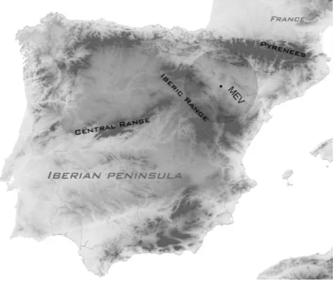
The middle Ebro Valley (MEV) in the northeast of the Iberian Peninsula is one of the areas in Europe with high-est frequency of hail events, with about 60 days character-ized by storms each summer (López and Sánchez, 2009). Since 2001, the Atmospheric Physics Group (GFA) of the University of León in Spain has been developing a number of projects in this area to study hailstorm convection and monitor its development (García-Ortega et al., 2007, 2011; Sánchez et al., 2009). The GFA uses a C-band weather radar system with a nowcasting model for detection of hailstorms (NMDH) (López and Sánchez, 2009). However, this hail de-tection system has some drawbacks, such as limited spatial range and radar beam shielding in mountainous areas. The aim of the present study is to develop a tool for identify-ing hail storms in real time that avoids the drawbacks of the radar system. Thus, the aim was to develop a nowcasting tool to identify hail-bearing clouds using MSG data. Its temporal resolution (15 min in operational mode) is lower than that of the radar (4 min for the University of León radar), but it may be used to monitor convection in real time.

To meet this objective, a hail detection tool (HDT) has been developed in two steps using logistic regression mod-els. First, the deep convection is identified using a convective mask algorithm (CM); second, the hail mask algorithm (HM) is used to identify hail precipitation within the clouds. This system was applied in the summer months (June, July and August) during daylight hours (with solar zenith angle lower than 70◦), when hailstorms are most frequent in the study area.

2 Study area and nowcasting model for detection of hailstorms

(3)

Fig. 1. Study area map. Circled area shows GFA radar range.

85 % and false alarm ratio (FAR) of 15 %. Therefore, this tool determines the presence or absence of hail and predicts the spatial likelihood of hail precipitation for each storm de-tected by the radar.

In this paper, the results of the NMDH have been used as “ground truth” for the construction of the training and valida-tion databases of HDT. The reason for this is the accuracy of this tool in identifying hail precipitation (López and Sánchez, 2009). Furthermore, it is possible to determine to some extent the time of hail precipitation events. Given the small spatial and temporal scales of these events, determining the exact time is important. Nevertheless, it was decided not to use di-rect observation of hail data on the ground from the observer network, as these reports have larger time uncertainties.

3 The logistic regression method

Logistic regression is a widely used statistical tool in mete-orology and land use studies (Applequist et al., 2002; Bas-tarrika et al., 2011; López et al., 2007). Sections 4.2 and 5.2 describe construction of two logistic regression models for formulating the CM and HM algorithms. The present section describes basic features of the logistic regression technique applied in the study. The technique provides probability of occurrence (P) of a particular weather event (categorical able) from values of a number of metric explanatory vari-ables (Xk). When the categorical variable is dichotomous, binary logistic regression is used. When there are more than two values involved, the latter is substituted by multinomial logistic regression (Hosmer and Lemeshow, 1989). The P obtained by the model for a categorical variable of the two

Table 1. List of channels of SEVIRI (Schmetz et al., 2002) used as

explanatory variables in CM and HM.

Channel Characteristics of spectral band (µm)

λmin λcen λmax

VIS0.6 0.56 0.635 0.71

VIS0.8 0.74 0.81 0.88

NIR1.6 1.50 1.64 1.78

IR3.9 3.48 3.90 4.36

WV6.2 5.35 6.25 7.15

WV7.3 6.85 7.35 7.85

IR8.7 8.30 8.70 9.10

IR9.7 9.38 9.66 9.94

IR10.8 9.80 10.08 11.80

IR12.0 11.00 12.00 13.00

IR13.4 12.40 13.40 14.40

groups is expressed as follows:

P1(X1, X2. . . Xk)=p1=

exp(Z1)

1+exp(Z1)

, (1)

P2(X1, X2. . . Xk)=p2=1−p1=

1 1+exp(Z1)

, (2)

whereZ1=α+

k X

j=1

βjXj; Xjforj=1, . . ., kare the metric explanatory variables;k is the total number of variables or interactions between variables included in the model;α is the intercept;βj for j=1, . . ., k the various discriminating coefficients; andPn represents the probability of belonging to group (1) or group (2), which ranges between 0 and 1. Note thatp1+p2=1.

(4)

is the scientific path to assess an equation formulated using a strictly statistical method.

The logistic regression model can be improved by intro-ducing interactions between the predictor variables, thereby increasing the predictive power of the equations. In this study, the model was constructed by introducing first-order interactions between the metric explanatory variables. Thus, data from a particular MSG channel may be input individu-ally or combined with those from another channel. The pres-ence of interactions causes the relation between the categor-ical variable and metric explanatory variable to depend on the value of a third variable. Thus, the contribution of each variable in the logistic model is conditioned by the variable with which it interacts. This fact complicates interpretation of the variables included in the model; however, it increases its predictive power significantly. The sign ofβ coefficients determines the sign of the contribution of each variable to the model, when there are no interactions, or also the interaction variable as a whole (Xm). In this case, a positiveβcoefficient involves greater probability in the model when the value of the variable increases, and the reverse is also true. When the variables show interactions they must be interpreted together physically, because in order to extract the sign of each single variable (Xj) it is necessary to combine theirβ coefficients (Eq. 3), which depend on the value of the variable with which it interacts (Xi):

SignXj =Sign(βj+βmXi), (3)

where Xj and Xi are single variables involved in the in-teraction, and Sign Xj is the sign of the contribution of this variable to the model. Xm is the interaction variable (Xm=XjXi) andβm is the interaction coefficient. As the interaction variable (Xm) has a high order of magnitude, it is necessary to provide the interaction β coefficient with a sufficient number of decimal points.

To check whether the explanatory variables added to the model have a high degree of statistical significance, global fitting of the model may be computed via the chi-squared test for variation of the value−2LL with respect to the base model (without variables). Thus, a model with good fit will have a large reduction for−2LL, and a perfect fit is one in which the likelihood is 1 and−2LL is zero. Owing to the in-troduction of the independent variables, the chi-squared test for assessing significance of the reduction of−2LL must be significant. In addition, several differentR2 measures have been constructed to represent a global fit of the model. Some of these measures are the Cox and Snell (Hair et al., 1999) and NagelkerkeR2 values (Hair et al., 1999); both are be-tween 0 and 1, and 1 is considered a perfect fit.

Finally, the Wald test was applied to assess the significance of the β coefficients for variables included in the logistic equation (Hair et al., 1999). Variables with significance of 0.1 may thus be interpreted as metric explanatory variables in discrimination of the categorical variable. It is important to point out that the greater the significance and Wald statistic

are, the greater weight the variable will have in the logistic model. The Wald statistic is used to compute the weight of each variable in the model instead of theβ coefficients, be-cause the metric explanatory variables have different orders of magnitude.

In accord with Hosmer and Lemeshow (1989), the cutoff point for discrimination between Eqs. 1 and 2 was fixed at 0.5, for both the CM and HM.

4 Convective mask

HDT consists of two distinct stages. First, the CM was set up to identify deep convection using MSG data. To do this, a database of cloud events was created and subsequently ana-lyzed from a microphysical point of view. These microphysi-cal and optimicrophysi-cal analyses of the various cloud types were stud-ied to interpret the results of the logistic model from a me-teorological perspective. Although there are numerous CMs for SEVIRI (Berendes et al., 2008; Henken et al., 2011), we opted to develop a new CM to verify the HDT in its entirety. However, other CMs for SEVIRI can be used as a basis for later application of the HM.

4.1 Database

The training database used to construct the CM included satellite imagery from the summer months between 2006 and 2010 during daytime (solar zenith angle lower than 70◦). Cloud types were identified using red-green-blue (RGB) combinations. These combinations enabled repre-senting physical information in the MSG channels (Lensky and Rosenfeld, 2008). Using the RGB compositions “day mi-crophysical”, “day solar” and “convective storms” by Lensky and Rosenfeld (2008), 700 events were classified, 100 for the following cloud types: cumulonimbus, stratocumulus, cirrus, nimbostratus, cirrostratus and multilayer cloud, stratus, and clear sky. An event was defined as an MSG image when cloud systems of the above-mentioned cloud types with a spatial extent of at least 10 km2could be identified by RGB combination. Only independent events were taken into ac-count, removing MSG images related to the temporal evolu-tion of the same cloud system.

(5)

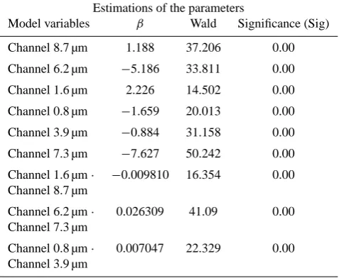
Table 2. Parameters selected by logistic regression for CM: metric

explanatory variables input to the model,βcoefficients used to ex-tract the sign, and Wald parameter used to compute the weight. The symbol “·” represents multiplication between variables.

Estimations of the parameters

Model variables β Wald Significance (Sig)

Channel 8.7 µm 1.188 37.206 0.00

Channel 6.2 µm −5.186 33.811 0.00

Channel 1.6 µm 2.226 14.502 0.00

Channel 0.8 µm −1.659 20.013 0.00

Channel 3.9 µm −0.884 31.158 0.00

Channel 7.3 µm −7.627 50.242 0.00

Channel 1.6 µm· −0.009810 16.354 0.00 Channel 8.7 µm

Channel 6.2 µm· 0.026309 41.09 0.00 Channel 7.3 µm

Incercept (α) = 1492.636

green = 1.6 µm; blue = 3.9 µm reflectance) is very sensitive to cloud microphysics and serves to determine the particle size and phase at the cloud top. Finally, the “convective storms” scheme (red = BT difference 6.2–7.3 µm; green = BT differ-ence 3.9–10.8 µm; blue = reflectance differdiffer-ence 1.6–0.6 µm) highlights clouds with very cold tops and allows better iden-tification of young, severe storms. Thus, convective clouds characterized by strong updrafts that appear bright yellow can be distinguished from cumulonimbus clouds with large ice particles, which show up as red (Lensky and Rosenfeld, 2008). Uncertainty in the detection of each type of cloud via these schemes has been reduced by combining information from the various RGB schemes used.

For the total 700 identified events, radiances and re-flectances of the MSG channels were retrieved for each event at 15 min temporal resolution . The reflectances were trans-formed into albedos following the Lambert method to avoid their dependence on solar zenith angle, and the radiances were transformed into BTs. The 3.9 µm radiances were con-verted to BT, taking both contributions into account. It is im-portant to point out that surfaces with high reflectances in the direction of the satellite may have albedos greater than 100 %. Only albedos and BTs of different MSG channels were then used as inputs in building the logistic regression model.

4.2 Results of logistic regression

As mentioned in Sect. 2, logistic regression was used to con-struct the CM, with data from the first 11 MSG channels chosen as explanatory variables (Table 1) and the

categor-Table 3. Parameters of the global fit of the model for the CM.

Chi-squared test for−2LL reduction and severalR2measures.

Information of the global fit

R2contrasts Likelihood ratio contrasts

Cox and Snell Nagelkerke −2 log likelihood Chi-squared Sig.

0.456 0.804 161.297 428.298 0.00

Table 4. Contingency table of database for CM.

Classification Forecast

Observed Convective-free Convective Correct percentage

Convective-free 591 9 98.50 %

Convective 12 88 88.00 %

Global percentage 85.80 % 14.20 % 97.00 %

ical variable represented by the presence (P1) or absence

(P2) of cumulonimbus clouds. Thus, albedos and BTs of 600

cumulonimbus-free events were input to the model, along with the cumulonimbus events, to find the combination of MSG channels that best distinguished these two groups sta-tistically. The binary logistic model is based on the forward stepwise method and executed over 10 iterations, introduc-ing 9 variables in Eqs. (1) and (2). The estimatedβ coeffi-cients gave a correlation coefficient equal to zero, according to Wald’s test (Table 2); thus, all are susceptible to physi-cal interpretation. Global fit of the model was assessed using the statistics described in Sect. 2. The chi-squared test used to assess the reduction of the−2LL parameter showed that it was significant (Sig<0.05), so the fit was satisfactory. In addition, the Nagelkerke’sR2 and the Cox and Snell’s R2 gave values of 0.456 and 0.804, respectively, which can be considered an acceptable fit (Hair et al., 1999) (Table 3).

Table 4 shows the classification of events included in con-struction of the logistic equation. A contingency table was built, and 700 events were classified according to the algo-rithm result. Of the 600 noncumulonimbus events included in the training set, only 9 were classified as cumulonimbus. Of the 100 cumulonimbus events, 12 were wrongly classified. The correct classifications were 97 %, with POD of 88 % and a FAR of 9 %.

4.3 Physical interpretation of results

To assist in physical interpretation of the logistic model re-sults, the cloud physical properties optical thickness (OT), effective radius (Re) and liquid water path (LWP) were

(6)

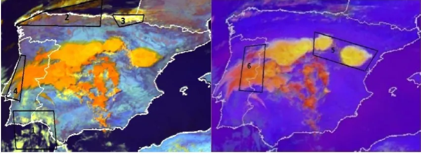
Fig. 2. 14:00 UTC on 12 August 2011. Left, RGB image “day solar”; right, RGB image “convective storm”. Different cloud types are marked.

1: stratus; 2: cirrus; 3: nimbostratus; 4: cirrostratus; 5: developing convection; 6: dissipating convection.

reflectance of clouds, since they determine the amount of ra-diation transferred to the surface, reflected and scattered to the satellite sensor, and the amount of radiation absorbed by the cloud layer. These characteristics vary according to cloud type (King et al., 1992).

4.3.1 Cloud physical properties: liquid water path, optical thickness and effective radius

The cloud physical properties were examined for a represen-tative case study, for example, from the event on 12 August 2011 at 14:00 UTC (Coordinated Universal Time). This is because at that time there were a variety of cloud types over the Iberian Peninsula. Figure 2 is the RGB image “day so-lar”, showing areas with stratus, nimbostratus, cirrus and cir-rostratus clouds. To the right of the figure, the RGB image “convective storm” highlights cumulonimbus clouds in dif-ferent stages of development.

The cloud physical properties were obtained for each cloud pattern and are described below.

a. LWP

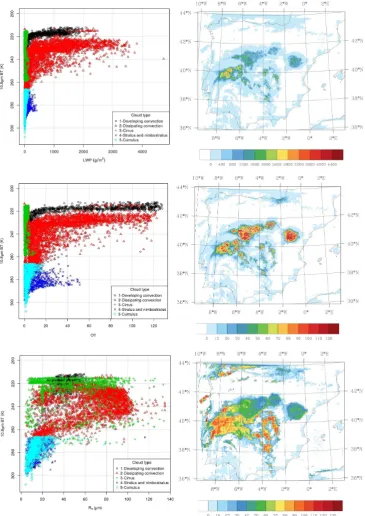
The scatter plot of LWP values as a function of BT (10.8 µm) for the various cloud types (Fig. 3, up-per panels) shows that cirrus and cirrostratus have the smallest LWP. Cumulus clouds with little devel-opment also had low LWP values, whereas stratus and nimbostratus are characterized by LWP values of up to 410 g m−2, despite their relatively small thick-ness. Convective clouds showed the highest LWP, with many pixels having more than 1000 g m−2.

b. OT

The OT (Fig. 3, middle panels) shows that cirrus clouds had very low OT values, since they are nearly transparent. OT values increased for cumulus clouds with weak development and, in stratus and nimbo-stratus clouds, they neared 50, since these clouds are

opaque. Both developing and dissipating cumulonim-bus clouds had the highest OT values (128 in this ex-ample), with no major differences between the two. c. Re

TheRescatter plot (Fig. 3 bottom panels) shows that

cloud tops below the glaciated zone had lowRe

val-ues, as with stratus and developing cumulus clouds. In contrast, cloud tops containing ice crystals had much higher values. For strong convection in the developing stage,Revalues were not particularly high compared

to convection in the dissipating stage. This is due to the fact that updrafts within convective clouds in the devel-oping stage are much stronger and, as a result, hetero-geneous nucleation produced in the mixed phase does not have enough time to form large ice crystals. Thus, smaller ice particles are formed via homogeneous ice nucleation above the level of glaciation compared to particles of greater size formed via heterogeneous nu-cleation (Rosenfeld et al., 2008).

The microphysical properties of the different cloud types were investigated to determine features that enable distinc-tion between convective and other cloud events. Cumulonim-bus clouds are characterized by high LWP, high OT values and, depending on their stage of development, variableRe

values. Thus, albedos and BTs included in the logistic model should reflect these characteristics.

4.3.2 Model input variables

(7)

Fig. 3.Left: Scatter plot of LWP (top), OT (middle) andRe(bottom) values as a function of 10.8-µm BT for

the cloud types at 1400 UTC, 12 August 2011. Right: LWP (top), OT (middle) andRe(bottom) over Iberian

Peninsula.

25

Fig. 3. Left: scatter plot of LWP (top), OT (middle) andRe(bottom) values as a function of 10.8 µm BT for the cloud types at 14:00 UTC, 12 August 2011. Right: LWP (top), OT (middle) andRe(bottom) over the Iberian Peninsula.

– Channels at 6.2 and 7.3 µm, and their interaction

(channel 6.2 µm×channel 7.3 µm): emission in this part of the spectrum occurs within the water va-por (WV) absorption band. The channel at 6.2 µm is sensitive to WV emittance in the upper tropo-sphere, and that at 7.3 µm to emittance in the

(8)

troposphere, and this is a crucial feature for identify-ing this cloud type. These clouds produce high LWP values and low BTs in the WV channel spectrum. To-gether, these three variables are inversely correlated with high probabilities of cumulonimbus, so low BTs in the 6.2 and 7.3 µm channels are associated with high probability of cumulonimbus, which accords with physical expectations.

(channel 8.7 µm×channel 1.6 µm): the channel with the next-highest weight in the model is of 8.7 µm (Wald parameter in Table 2). The interpretation of this channel in the model has been carried out con-sidering its category (infrared windows). This means that introducing new channels of the same category does not lead to a statistically significant improve-ment in the model. This fact was checked by sub-stituting the 8.7 µm channel with other infrared win-dow channels (at 10.8 and 12 µm). The results of this new model were very similar to the original, after ad-justing the coefficient. The atmospheric window chan-nels permit distinction between different cloud top temperatures. Developing cumulonimbus clouds have tops formed by ice crystals near the tropopause, and the channel therefore distinguishes them from middle and low clouds. The channel with which it interacts (1.6 µm), albeit with less weight in the model, permits distinguishing the cloud-top phase. At 1.6 µm, ice and liquid-water clouds have very different reflectances (Cattani et al., 2007; Rosenfeld et al., 2008), owing to sensitivity toReand cloud phase. Cloud tops formed

by liquid-water hydrometeors have lower absorption than those formed by ice crystals, so reflectances are higher for water than for ice particles. In this case, the signs of the variables are related. To extract these signs, it is necessary to combine their β coefficients (Table 2) using Eq. 3. Thus, channel 1.6 µm has a positive effect for channel 8.7 µm BTs of less than 226.91 K, and a negative effect for BTs greater than that value. This result has a physical interpretation, since clouds with 8.7 µm BTs of less than 226.91 K (lower than the level of homogeneous nucleation, ac-cording to Rosenfeld et al. (2008)) are formed by ice crystals. Greater albedo values at 1.6 µm mean that particles at cloud top are small, and updrafts are more vigorous (Rosenfeld et al., 2008); that is, the probabil-ity of cumulonimbus increases. On the contrary, clouds with 8.7 µm BTs warmer than this temperature may be formed by liquid water, with large albedos at 1.6 µm, which diminishes the probability of cumulonimbus.

– Channels at 3.9 and 0.8 µm, and their interaction (

channel 3.9 µm×channel 0.8 µm): the channel with the next-highest weight in the model is at 3.9 µm (Wald parameter in Table 2). BTs in this channel, together

with those measured in channel 1.6 µm, are very sensi-tive toReat cloud tops (Cattani et al., 2007; Rosenfeld

et al., 2004). Cloud tops formed by water or small ice hydrometeors have low absorption and thus high BT. This fact enables distinguishing between clouds with tops characterized by low Re values and high TB in

this channel, and those with tops associated with high Revalues and low BT. This channel interacts with the

0.8 µm channel and, according to Nakajima and King (1990), reflectances at this wavelength depend primar-ily on cloud OT. As a result, this channel distinguishes between very dense, opaque clouds and thinner, trans-parent clouds. The interaction between these two chan-nels couples the effects ofReand OT, and their

infor-mation can be used for simultaneous retrieval of OT and Re (King et al., 1992). Mecikalski et al. (2010)

showed that changes in the reflectances of these chan-nels were related to the variations of OT and hydrome-teor size in growing clouds. The sign of the variables in the model also varies. Combining theirβ coefficients (Eq. 3), the 0.8 µm channel has a positive effect over the entire range of possible values of the 3.9 µm chan-nel. In other words, a large albedo at 0.8 µm produces large OT and a greater probability of cumulonimbus. The 3.9 µm channel has a positive effect for 0.8 µm channel albedos greater than 125.44 %, and a nega-tive effect for lesser albedos. The physical reason is similar to that explained in the second point above. Albedos greater than 125 % are typical of very dense clouds and, since BTs increase in the 3.9 µm channel, the probability of cumulonimbus increases. According to Mecikalski et al. (2010), reflectances in the visible channels do not provide definitive information about cloud top character, but they can be used to confirm that the cloud is optically thick and the use of 3.9 µm is acceptable.

As mentioned above, the CM uses a large number of vari-ables within the discriminating equation. This is because of the wide range of cloud types included in the database. How-ever, all channels selected using statistical criteria have an ad-equate physical interpretation in cloud-type discrimination. The results reveal that the “ingredients” required to distin-guish cumulonimbus clouds from other cloud types are, in order of importance, as follows:

– water vapor in the troposphere (assessed by the WV

channels),

– thermodynamic phase of particles at cloud top and top

cloud temperature (assessed by the NIR channels and the 8.7 µm channel), and

– cloud optical thickness and size of the particles at

(9)

Cumulonimbus clouds are thick, with a high WV concen-tration throughout the troposphere, and their cloud tops are formed by ice crystals. The combination of all these features enables discriminating this cloud type from others, and so these are the three “ingredients” that must be included in an algorithm for detecting cumulonimbus clouds. These ingre-dients are linked to the aforementioned physical properties. WV concentration, for example, is related to LWP. The ther-modynamic phase of the cloud is related toRe, since this

parameter strongly depends on the presence of ice or water.

5 Hail mask algorithm

The second step in construction of the HDT from MSG data is identification of hydrometeors within cumulonimbus clouds detected by the CM. The method for building the HM is similar to that described above for the CM. First, a database of cumulonimbus events was created, with and without hail. Then, the logistic regression model was constructed using the albedos and BTs to determine the MSG channels that best distinguish the hail events. Finally, microphysical and opti-cal cloud properties were studied in areas with hail to inter-pret the MSG channels included in the model from a physical perspective.

5.1 Database construction

The database for the HM was built using information from the GFA weather radar. This database includes daytime events recorded in the summer months, during five observa-tion campaigns between 2006 and 2010. To distinguish hail-bearing from hail-free events, the results of the NMDH im-plemented for the radar data (López and Sánchez, 2009) were used. The NMDH provides the likelihood of hail precipita-tion, and its results were considered "ground truth" data. A hail pixel is one at which the likelihood of hail according to the NMDH exceeds 90 %. To build the database using radar data, the following issues were taken into account.

– Temporal resolution. The radar data must correspond

to the same time span of the MSG satellite scan across the study area. In this case, for the MEV the satellite gathers data between 8.5 and 9 min after the scan initi-ation.

– Parallax effect. The parallax effect is important for the

MSG because the satellite is above the Equator, tak-ing measurements of Europe at relatively low angles. Lábó et al. (2007) found a deviation up to four pixels towards the southwest for high clouds over Hungary. The MEV is not situated at the satellite nadir and the analyzed cumulonimbus clouds have high tops; thus, correction must be done. The deviations computed in this study follow the method of Vicente et al. (2002), which takes data of cloud-top height from vertical re-flectivity profiles obtained by the radar. For example,

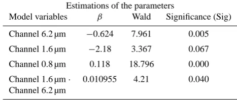
Table 5. Parameters selected by logistic regression for HM: metric

explanatory variables input to the model,βcoefficients used to ex-tract the sign, and Wald parameter used to compute the weight. The symbol “·” represents multiplication between variables.

Estimations of the parameters

Model variables β Wald Significance (Sig)

Channel 6.2 µm −0.624 7.961 0.005

Channel 1.6 µm −2.18 3.367 0.067

Channel 0.8 µm 0.118 18.796 0.000

Incercept (α) = 115.039

for high clouds (between 15 and 18 km) the deviations reached 18 km to the south; there were very small de-viations in the E-W direction, because the zero degree meridian crosses the study area. Eventually, this cor-rection enables comparing satellite and radar data at the same surface location.

– Spatial resolution. The GFA radar data have a

resolu-tion of 0.75 km, whereas the MSG data have spatial sampling distance of 3 km at the subsatellite point. Be-cause of this and considering small deviations of hail precipitations that may be attributed to wind, we con-sidered only hail precipitation with an extent of at least 18 radar pixels. In this case, an event is defined as a cumulonimbus with a spatial extent of at least 10 km2 identified in radar images pertaining to independent convective cells.

The hail training database was thus constructed, with the fol-lowing events:

– 100 events of precipitating cumulonimbus clouds with

hail,

– 50 events of precipitating cumulonimbus clouds

with-out hail, and

– 50 anvil clouds.

Finally, radiances or reflectances of the first 11 MSG chan-nels were considered for each event (Table 1). These were transformed into BTs and albedos, respectively, as with the CM algorithm.

5.2 Results of logistic regression

(10)

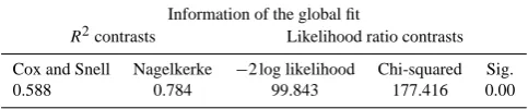
Table 6. Parameters of global fit of the model for HM. Chi-squared

test for−2LL reduction and severalR2measures.

Information of the global fit

R2contrasts Likelihood ratio contrasts

Cox and Snell Nagelkerke −2 log likelihood Chi-squared Sig.

0.588 0.784 99.843 177.416 0.00

Table 7. Contingency table for HM database.

Observed Hail-free Hail Correct percentage

Hail-free 93 7 93.00 %

Hail 8 92 92.00 %

in the equation. Theβ coefficients estimated for each vari-able are significant (Sig<0.1) for physical interpretation, according to Wald’s test (Table 5). Global fit of the model was assessed through the statistics described in Sect. 2. The chi-squared test used to assess reduction of the −2LL pa-rameter yielded significant results (Sig<0.05), revealing a good fit for the model. In addition, Nagelkerke’s R2 and Cox and Snell’sR2indicators yield 0.784 and 0.588, respec-tively, demonstrating an acceptable fit (Hair et al., 1999) (Ta-ble 6). Ta(Ta-ble 7 shows the classification of events included in the construction of the logistic equation. A contingency table was built, classifying the 200 events according to the model. Among the 100 hail-free events, only seven were wrongly classified. Among the 100 hail events, eight were wrongly classified. Correct classification amounted to 92.5 %, with POD 92 % and FAR 7 %.

5.3 Physical interpretation of results

As in the case of the CM, the cloud physical properties OT, LWP andRe were extracted from the VISST algorithm for

a sample case study, to make a proper physical interpreta-tion of the MSG channels selected by the model. The aim was to determine microphysical characteristics in areas with and without hail. To study these properties, several single-cell storms were chosen. The NMDH was used to identify storm areas with high likelihood of hail precipitation. Then, scatter plots of the cloud properties as a function of corre-sponding cloud-top temperatures were used to compare these hail sectors with others within the cumulonimbus cloud.

5.3.1 Cloud physical properties: liquid water path, optical thickness and effective radius

The scatter plots were constructed by selecting convec-tive areas identified by the CM in the sample case study (14:00 UTC, 12 August 2011). Areas affected by hail are

Table 8. Average results of algorithms for the 26 events of each

type included in the verification database. CM shows cumulonim-bus probability and HM hail precipitation probability.

CM HM

Hail cumulonimbus 99.34 68.43 Free-hail cumulonimbus 80.63 29.82 Free cumulonimbus 4.09 0.05

shown by black contours (Fig. 4). The radar only covers the northeast of the study area (red circle in figure), so hail areas outside of this coverage are not identified.

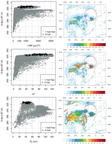
a. LWP

The LWP (Fig. 4, upper panels) did not reveal major differences between hail and hail-free areas. Neverthe-less, whereas clouds without hail and lower heights ex-hibit a wide range of LWP values of up to 3000 g m−2_,

clouds with hail have smaller LWP values. For hail ar-eas, most of the water vapor is transported by strong updrafts toward upper levels in the cloud, forming ice. However, in other parts the cloud is affected by down-drafts and, thus, there are significant accumulations of liquid water at the base, thereby increasing the LWP. b. OT

The OT (Fig. 4, middle panels) shows that the hail ar-eas were mostly in regions with OT between 40 and 100. It is seen that many cloud pixels not associated with hail precipitation also have high OT values, be-cause the anvil has high values.

c. Re

The Re (Fig. 4, bottom panels) shows that most hail

pixels had Re between 30 and 50 µm, considerably

smaller than values at other cold pixels. This represents the microphysical property that best discriminates hail and hail-free regions within a cloud. In hail areas, up-drafts are stronger than in other parts of the cloud, and lowerRevalues are found.

5.3.2 Variables input to the model

Channels included in the logistic equation are shown in Table 5. A physical interpretation of the variables, along with their interactions in order of weight in the model according to the Wald statistics, is shown below.

– Channel at 0.8 µm: this channel with a positive effect

(11)

Fig. 4.Left: LWP (top), OT (middle) andRe(bottom) as in Fig. 3 for hail (black) and no hail (gray) pixels.

Right: LWP (top), OT (middle) andRe(bottom), black lines correspond to areas with high likelihood of hail

according to radar. Circled area shows radar range. ₂₆

Fig. 4. Left: LWP (top), OT (middle) andRe(bottom) as in Fig. 3 for hail (black) and no hail (gray) pixels. Right: LWP (top), OT (middle) andRe(bottom), black lines correspond to areas with high likelihood of hail according to radar. Circled area shows radar range.

a V-shaped form. Bedka (2011) found that 53 % of cumulonimbus with overshooting clouds produce hail on the ground. To detect this type of structure it is necessary to apply techniques of spatial recognition, since the present method using a pixel-by-pixel anal-ysis does not permit such detection. However, it has been observed that these structures have high albedos in the visible and NIR channels (Berendes et al., 2008). Thus, pixels with elevated albedos in the 0.8 µm chan-nel must be considered for hail identification.

How-ever, apart from the visible channels, additional chan-nel information is necessary for this detection (Beren-des et al., 2008).

(12)

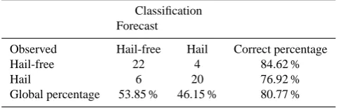
Table 9. Contingency table for verification of HDT by

cumulonim-bus events in summer 2011.

Observed Hail-free Hail Correct percentage

Hail-free 22 4 84.62 %

Hail 6 20 76.92 %

(Table 5) in Eq. 3). Channel 1.6 µm has a positive effect for BTs greater than 198.99 K at 6.2 µm. In the train-ing database, none of the episodes identified as cumu-lonimbus via the CM had albedo values greater than 56.96 % at 1.6 µm or BT less than 198.99 K at 6.2 µm. Thus in practice, channel 6.2 µm will have a negative sign and channel 1.6 µm a positive sign. The probabil-ity of hail increases with albedo in the 1.6 µm channel and BT diminishes in the 6.2 µm channel, consistent with physical expectations. Storms can produce hail in their developing stage when their mass centroids are in the upper layers (López and Sánchez, 2009). This results in high WV concentrations in the upper tropo-spheric layers, producing a decrease in BTs at 6.2 µm. Channel 1.6 µm does not have the greatest weight in the equation; however, it is fundamental for hail de-tection. Its reflectances are associated with ice particle size, since cloud tops formed by liquid water are fil-tered by the CM.

As seen in the analysis of microphysical cloud properties, hail areas have small ice particles at their cloud tops because of the strong updrafts. It is well known that presence of hail on the ground is directly related to updraft speed (López et al., 2000). This speed determinesRe at cloud tops

(Rosen-feld et al., 2008). Therefore, reflectances in this channel are higher than those in regions with large ice particles. These results reveal that the ingredients necessary for discriminat-ing regions with hail precipitation within cumulonimbus are, in order of importance, as follows:

– optical thickness (assessed by the visible channels),

– water vapor in upper troposphere (assessed by the WV

channel), and

– speed of updrafts (assessed by the NIR channels).

The combination of all these ingredients discriminates hail sectors from the remainder of the cumulonimbus cloud.

6 Verification of HDT from MSG data

The HDT was verified with convective hail events recorded in the MEV during summer 2011, since these data were not included in the initial training database.

Table 10. Skill scores for verification contingency table.

Calcula-tion follows method of López and Sánchez (2009).

Skill scores Acronyms Value

False alarm ratio FAR 16.7 %

Frequency of hits FOH 83.3 %

Frequency of misses FOM 23.1 %

Probability of detection POD 76.9 % Probability of null event PON 84.6 % Probability of false detection POFD 15.4 % Detection failure ratio DFR 21.4 % Frequency of correct null events FOCN 78.6 %

Heidke’s skill score HSS 0.640

True skill score TSS 0.615

6.1 Database

The same procedure as that chosen to extract hail events us-ing the NMDH (no direct ground measurements) was fol-lowed to build the verification database. Hail-free events were either associated with convective clouds with tops higher than 10 km and with liquid precipitation registered on the ground of various intensities (radar-measured), or with parts of the anvil of the convective cloud. The verification database includes the following events:

– 26 convective-free events (cirrus, cirrostratus,

stra-tocumulus, stratus and blue-sky),

– 26 hail events corresponding to convective cells (one

or more cells), and

– 26 hail-free events (rain of varying intensities and

anvil).

The database constructed using these radar data was con-sidered ground truth. To assess the HDT results, we need to compare probabilities obtained by the model built using MSG data and the ground truth data for each event. Spa-tial probability weighting was used for this comparison. For each event, the central MSG pixel was extracted together with eight surrounding pixels, and the maximum likelihood among all nine MSG pixels was considered. The reason for this spatial weighting is that data from the MSG pixel might not coincide exactly with hail recorded on the ground. De-viations may occur, one source of these being the error in cloud-top estimation with the radar, and another the compu-tation of the parallax effect. Other deviations may be from strong wind shear, which can tilt the storm. In all these cases, the area on the ground where hail is recorded does not coin-cide exactly with the cloud top.

6.2 Results

(13)

Fig. 5. 12 August 2011. Left: radar-based accumulated hail likelihood for entire day in MEV. Right: radar-based hail likelihood at 14:00 UTC.

Convective cells with high hail likelihood are marked in red. Circled area shows the 100 km radar range

Fig. 6. 14:00 UTC on 12 August 2011. Left: convective areas delineated by CM. Right: HDT outputs in terms of hail probability.

model construction. Validation was done for the HDT over-all. The verification of the CM for cumulonimbus detection shows that of the 52 cumulonimbus events analyzed, the CM identified 48 correctly. Only four cases were considered non-convective, none of which produced hail precipitation. In ad-dition, only one cumulonimbus-free event (cirrostratus) out of 26 such events included in the verification database was erroneously classified as cumulonimbus. This was later cor-rectly filtered by the HM. It can therefore be said that the CM does not filter out any hail event.

Table 8 shows average likelihoods of the two algorithms for the 26 events of each type included in the verification

database. For the CM, greater likelihoods were obtained for the cumulonimbus events, with a likelihood near 100 % for hail events. The HM revealed great sensitivity, with a large difference between hail and hail-free cumulonimbus events. The two algorithms gave very low likelihoods for the cumulonimbus-free events. Once it was shown that none of the cumulonimbus-free events were classified as hail, the ver-ification focused on convective episodes.

(14)

well-developed convective clouds generating intense rainfall (greater than 30 dBz radar reflectivity). Moreover, six hail events were wrongly classified as nonhail events.

Skill scores were computed using data from the contin-gency table to investigate different aspects of model validity. Table 10 shows a POD of 76.9 % and FAR of 16.7 %, both satisfactory values. Heidke’s skill score (HSS) and true skill score (TSS) were also computed. For both indices, a value of 1 is considered a perfect forecast.

These results are slightly worse than those achieved by the radar-based hail-detection algorithms. However, the advan-tages of using satellite data instead of radar data make this approach valuable for monitoring hailstorms.

6.3 Application of the HDT: case study on 12 August 2011

The model was applied to the case study at 14:00 UTC on 12 August 2011. The synoptic situation showed a low pressure center at 500 hPa with strongly convergent flow at the sur-face. This center moved from the southwest of the Iberian Peninsula to the northeast. There was an isolated cold air mass in the upper tropospheric layers (−10◦C at 500 hPa), with strong warm and moist advection in lower layers. These meteorological conditions favored development of intense storms over the peninsula. In fact, the initial storms to the west-southwest of the peninsula were detected around noon. Shortly afterward, more storms developed over the Iberian and Central Mountain systems. Figure 5 shows areas with high likelihoods of accumulated hail as derived by radar dur-ing the day in the MEV. The Iberian range was the area most widely affected by hail.

At 14:00 UTC there were several convective cells over the central peninsula, in different stages of development. In the north, nearly transparent cirrus and nimbostratus clouds were detected over the eastern coast. In the southwest of the penin-sula there were stratus clouds (Fig. 2). The radar in the MEV showed a number of storm cells with high hail likelihood over the province of Teruel (Fig. 5). To the west of the Iberian Mountain system, lower likelihoods of hail were evident, but this might be a result of poor radar coverage because of the long distance .

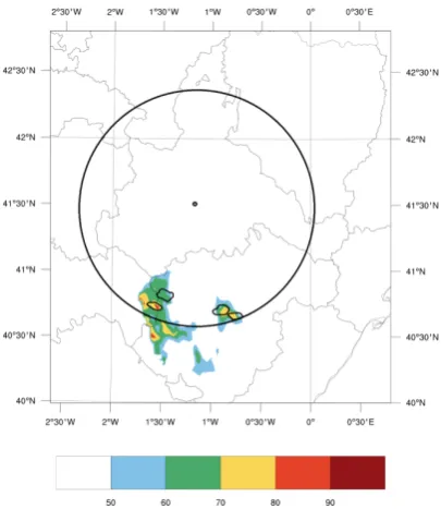
The result of applying the CM and HM to the case study is shown in Fig. 6. The HDT results are shown on a proba-bility scale, and are obtained by applying the HM to pixels identified as cumulonimbus by the CM (using a threshold of 50 %). Convective cells were detected with high hail like-lihood in the southern Iberian Mountain system and around the Central Mountain system. These areas also agree with the radar for hailstorm presence (Fig. 7).

Fig. 7. 14:00 UTC on 12 August 2011. Color scale: HDT outputs in

terms of hail probability. Black contours: radar-based hail precipi-tation. Circled area shows the 110 km radar range.

7 Conclusions

A daytime HDT was introduced for the summer months, us-ing MSG data and applyus-ing two logistic regression models. The stepwise method was used to input variables for algo-rithm definition, with first-order interaction between the pre-dictive variables. The CM identifies convective cloud pixels, whereas the HM discriminates pixels with hail precipitation from other convective cloud pixels.

The following conclusions can be drawn.

– The CM includes nine explanatory variables.

Meteoro-logical interpretation of these variables reveals that the “ingredients” required to discriminate cumulonimbus clouds from other cloud types are as follows: WV in the troposphere (assessed by the WV channels), ther-modynamic phase of particles at cloud top and cloud-top temperature (assessed by the NIR channels and channel 8.7 µm), and cloud thickness and size of parti-cles at cloud top (assessed by channel 0.8 µm and NIR channels).

– The HM includes four explanatory variables.

(15)

– Preliminary application of the CM is crucial to filter

cloud tops formed by liquid water. The reason is that the HM is very sensitive to values from the NIR chan-nels. Cloud tops formed by liquid water have smallRe

values and high reflectances in the NIR, so they would eventually be classified as hail.

– Analysis of the cloud physical properties indicated that

cumulonimbus clouds are characterized by high LWP and OT values, plus varyingRevalues, depending on

the stage of cell development. The occurrence of hail within cumulonimbus clouds is linked to lowerRe

val-ues (30–50 µm) of particles at cloud top. Also, OT and LWP were not particularly useful parameters for iden-tifying hail within a convective structure.

– Validation of the HDT, using independent data from

2011, gave a POD of 76.9 % and FAR of 16.7 %. Although these results are slightly worse than those char-acterizing hail detection from ground-based radars, the HDT is recommended for application to areas with spatially lim-ited radar coverage . The HDT will be used for tracking and nowcasting of hailstorms in real time, using radar data to im-plement the system. Finally, the effective spatial and tempo-ral coverage of this tool will allow recording of hailstorms in the Iberian Peninsula in a database, for in-depth investigation of regional hail climatology.

Acknowledgements. This study was funded by research projects awarded by the Junta de Castilla y León: LE220A11-2, LE003B009 and LE176A11-2. The authors wish to thank the Department of Education of the regional government Junta de Castilla y León and the European Social Fund (ORDEN EDU/1064/2009, 14 May) for providing funding for recently graduated students cooperating in the study. Cloud properties from MSG were kindly provided by P. Minnis and his group (http://www-pm.larc.nasa.gov/). Two of the authors (E. Cattani and V. Levizzani) wish to acknowl-edge the EUMETSAT Satellite Application Facility on Support to Operational Hydrology and Water Management (H-SAF, http://hsaf.meteoam.it/).

Edited by: G. Panegrossi

Reviewed by: two anonymous referees

References

Applequist, S., Gahrs, G. E., and Pfeffer, R. L.: Comparison of methodologies for probabilistic quantitative precipitation fore-casting, Wea. Forefore-casting, 17, 783–799, 2002.

Adler, R. F., Markus, M. J., Fenn, D. D., Szejwach, G., and Shenk, W. E.: Thunderstorm top structure observed by aircraft over-flights with an infrared radiometer, J. Appl. Meteor., 22, 579– 593, 1983.

Bastarrika, A., Chuvieco, E., and Martín, M. P.: Mapping burned areas from landsat TM/ETM+ data with a two-phase algorithm:

Balancing omission and commission errors, Rem. Sensing Env., 115, 1003–1012, 2011.

Bedka, K. M., Brunner, J., Dworak, R., Feltz, W., Otkin, J., and Greenwald, T.: Objective satellite-based detection of overshoot-ing tops usovershoot-ing infrared window channel brightness temperature gradients, J. Appl. Meteor. Climatol., 49, 181–202, 2010. Bedka, K. M.: Overshooting cloud top detections using MSG

SE-VIRI Infrared brightness temperatures and their relationship to severe weather over Europe, Atmos. Res., 99, 175–189, 2011. Berendes, T. A., Mecikalski, J. R., MacKenzie, W. M., Bedka,

K. M., and Nair, U. S.: Convective cloud identification and classification in daytime satellite imagery using standard devia-tion limited adaptive clustering, J. Geophys. Res., 113, D20207, doi:10.1029/2008JD010287, 2008.

Cattani, E., Melani, S., Levizzani, V., and Costa, M. J.: The re-trieval of cloud top properties using VIS-IR channels, in: Mea-suring Precipitation from Space – EURAINSAT and the Future, edited by: Levizzani, V., Bauer, P., and Turk, F. J., Springer, 79– 96, 2007.

Cattani, E., Torricella, F., Laviola, S., and Levizzani, V.: On the statistical relationship between cloud optical and microphysical characteristics and rainfall intensity for convective storms over the Mediterranean, Nat. Hazards Earth Syst. Sci., 9, 2135–2142, doi:10.5194/nhess-9-2135-2009, 2009.

Dworak, R., Bedka, K., Brunner, J., and Feltz, W.: Comparison be-tween GOES-12 overshooting-top detections, WSR-88D radar reflectivity, and severe storm reports, Wea. Forecast., 27, 684– 699, 2012.

Doswell, C. A. and Schultz, D. M.: On the use of indices and pa-rameters in forecasting severe storm, Electronic J. Severe Storm Meteor., 1, 1–14, 2006.

Doswell, C. A., Brooks, H. E., and Maddox, R. A.: Flash flood fore-casting: an ingredients-based methodology, Weather Forecast., 11, 560–581, 1996.

García-Ortega, E., López, L., and Sánchez, J. L.: Atmospheric pat-terns associated with hailstorm days in the Ebro Valley, Spain, Atmos. Res., 100, 401–427, 2011.

García-Ortega, E., Fita, L., Romero, R., López, L., Ramis, C., and Sánchez, J. L.: Numerical simulation and sensitivity study of a severe hailstorm in northeast Spain, Atmos. Res., 83, 225–241, 2007.

Hair Jr., F. J., Anderson, E. E., Tatham, R., and Black, W. C.: Análi-sis Multivariante, Prentice Hall, Madrid, 832 pp., 1999. Henken, C. C., Schmeits, M. J., Deneke, H., and Roebeling, R. A.:

Using MSG-SEVIRI cloud physical properties and weather radar observations for the detection of Cb/TCu clouds, J. Appl. Mete-orol. Clim., 50, 1587–1600, 2011.

Heymsfield, G. M., Szejwach, G., Schotz, S., and Blackmer Jr., R. H.: Upper-level structure of Oklahoma tornadic storms on 2 May 1979. II: Proposed explanation of V pattern and internal warm region in infrared observations, J. Atmos. Sci., 22, 1756– 1767, 1983.

Hosmer, D. W. and Lemeshow, S.: Applied Logistic Regression, Wiley Interscience, New York, 373 pp., 1989.

Inoue, T.: A cloud type classification with NOAA 7 split-window measurements, J. Geophys. Res., 92D, 3991–4000, 1987. Johns, R. H. and Doswell III, C. A.: Severe local storms forecasting,

(16)

King, M. D., Kaufman, Y. J., Menzel, W. P., and Tanré, D.: Remote sensing of cloud, aerosol, and water vapor properties from the MODerate Resolution Imaging Spectrometer (MODIS), IEEE T. Geosci. Remote, 30, 2–27, 1992.

Kurino, T.: A satellite infrared technique for estimating deep/shallow precipitation, Adv. Space Res., 19, 511–514, 1997.

Lábó, E., Kerényi, J., and Putsay, M.: The parallax correction of MSG images on the basis of the SAFNWC cloud top height prod-uct, in: Proceedings EUMETSAT Meteorological Satellite Conf. and 15th Satellite Meteorology and Oceanography Conf. Amer. Meteor. Soc., Amsterdam, the Netherlands, 2007.

Lensky, I. M. and Rosenfeld, D.: Clouds-Aerosols-Precipitation Satellite Analysis Tool (CAPSAT), Atmos. Chem. Phys., 8, 6739–6753, doi:10.5194/acp-8-6739-2008, 2008.

Levizzani, V. and Setvák, M.: Multispectral, high-resolution satel-lite observations of plumes on top of convective storms, J. Atmos. Sci., 53, 361–369, 1996.

López, L., Marcos, J. L., Sánchez, J. L., Castro, A., and Fraile, R.: CAPE values and hailstorms on northwestern Spain, Atmos. Res., 56, 147–160, 2000.

López, L., García-Ortega, E., and Sánchez, J. L.: A short-term fore-cast model for hail, Atmos. Res., 83, 176–184, 2007.

López, L. and Sánchez, J. L.: Discriminant methods for radar detec-tion of hail, Atmos. Res., 93, 358–368, 2009.

Marcos, C., and Rodriguez, A.: Algorithm Theoretical Ba-sis Document for “Precipitation products from Cloud Phys-ical Properties” (PPh-PGE14:PCPh v1.0 and CRPh v1.0) SAF/NWC/CDOP2/INM/SCI/ATBD/14, Issue 1, Rev. 0, July 2013.

Mecikalski, J. R., Mackenzie, W. M., König, M., and Muller, S.: Cloud-top properties of growing cumulus prior to convective ini-tiation as measured by meteosat second generation. Part II: Use of visible reflectance, J. Appl. Meteorol. Clim., 49, 2544–2558, 2010.

Mecikalski, J. R., Watts, P. D., and Koenig, M.: Use of Meteosat Second Generation optimal cloud analysis fields for understand-ing physical attributes of growunderstand-ing cumulus clouds, Atmos. Res., 102, 175–190, 2011.

Minnis, P., Kratz, D. P., Coakley Jr., J. A., King, M. D., Garber, D., Heck, P., Mayor, S., Young, D. F., and Arduini, R.: Cloud Op-tical Property Retrieval (Subsystem 4.3), Clouds and the Earth’s Radiant Energy System (CERES) Algorithm Theoretical Basis Document. Volume III: Cloud Analyses and Radiance Inversions (Subsystem 4), NASA RP 1376 vol. 3, CERES Science Team, 135–176, 1995.

Nakajima, T. and King, M. D.: Determination of the optical thick-ness and effective particle radius of clouds from reflected solar radiation measurements, Part I: Theory, J. Atmos. Sci., 47, 1878– 1893, 1990.

Rosenfeld, D., Woodley, W. L., Lerner, A., Kelman, G., and Lind-sey, D. T.: Satellite detection of severe convective storms by their retrieved vertical profiles of cloud particle effective ra-dius and thermodynamic phase, J. Geophys. Res., 113, D04208, doi:10.1029/2007JD008600, 2008.

Sánchez, J. L., Gil-Robles, B., Dessens, J., Martin, E., López, L., Marcos, J. L., Berthet, C., Fernández, J. T., and García-Ortega, E.: Characterization of hailstone size spectra in hailpad networks in France, Spain, and Argentina, Atmos. Res., 93, 641– 654, 2009.

Schmetz, J., Tjemkes, S. A., Gube, M., and Van de Berg, L.: Mon-itoring deep convection and convective overshooting with Me-teosat, Adv. Space Res., 19, 433–441, 1997.

Schmetz, J., Pili, P., Tjemkes, S., Just, D., Kerkmann, J., Rota, S., and Ratier, A.: An introduction to Meteosat Second Generation (MSG), B. Am. Meteorol. Soc., 79, 2457–2476, 2002.

Setvák, M., Lindsey, D. T., Novák, P., Wang, P. K., Radová, M., Kerkmann, J., Grasso, L., Su, S.-H., Rabin, R. M., Št’ástka, J., and Charvát, Z.: Satellite-observed cold-ring-shaped features atop deep convective clouds, Atmos. Res., 97, 80–96, 2010. Strabala, K. I., Ackerman, S. A., and Menzel, W. P.: Cloud

prop-erties infrared from 8–12 µm Data, J. Appl. Meteorol., 33, 212– 229, 1994.

Vicente, G. A., Davenport, J. C., and Scofield, R. A.: The role of orographic and parallax corrections on real time high resolution satellite rainfall rate distribution, Int. J. Remote Sens., 203, 221– 230, 2002.

(17)

Appendix A

Acronym list

BT: brightness temperature CM: convective mask FAR: false alarm ratio

GFA: Atmospheric Physics Group HDT: hail detection tool

HM: hail mask

HRV: high resolution visible LWP: liquid water path MEV: middle Ebro Valley

MSG: Meteosat Second Generation NIR: near-infrared

NMDH: nowcasting model for detection of hailstorms OT: optical thickness

POD: probability of detection Re: effective radius

RGB: red-green-blue

SEVIRI: Spinning Enhanced Visible and InfraRed Imager