University of Pennsylvania
ScholarlyCommons
Publicly Accessible Penn Dissertations
1-1-2016
Forest Biomass and Soil Carbon Stock Changes in
the Delaware River Basin
Bing Xu
University of Pennsylvania, icy6956@gmail.com
Follow this and additional works at:
http://repository.upenn.edu/edissertations
Part of the
Biogeochemistry Commons
,
Ecology and Evolutionary Biology Commons
, and the
Environmental Sciences Commons
This paper is posted at ScholarlyCommons.http://repository.upenn.edu/edissertations/2111
For more information, please contactlibraryrepository@pobox.upenn.edu.
Recommended Citation
Xu, Bing, "Forest Biomass and Soil Carbon Stock Changes in the Delaware River Basin" (2016).Publicly Accessible Penn Dissertations. 2111.
Forest Biomass and Soil Carbon Stock Changes in the Delaware River
Basin
Abstract
Forests play an important role in the global carbon cycle. Quantifying forest biomass and soil carbon stocks and their change over time and space is important to understand forest dynamics and their feedbacks with climate change. This dissertation investigates the forest biomass and soil carbon stocks and their controlling factors in the Delaware River Basin (DRB) using a combination of field measurements and modeling. In 2001-2003, 77 forest plots in three research sites were established and their biomass was measured. In 2012-2014, 61 of these plots were revisited and forest biomass was re-measured using the same protocols. Two soil sampling methods, the Forest Inventory Analysis standard soil core method and the quantitative soil pit method, were also used to collect soil samples. Based on the results of field measurements, a process-based ecosystem model (PnET-CN) was parameterized and used to simulate the spatial distribution of forest carbon pool and fluxes in the three sites. We found that the mean biomass carbon stock in the three sites was 166.5 Mg C ha-1 and had increased by 2.35 Mg C ha-1 yr-1 and was thus a carbon sink over the past decade. The soil carbon stock to 40 cm depth was 76.6 Mg C ha-1. The accuracy of the soil core sampling method was
questioned because in the surface mineral soil layer, lower bulk density, lower coarse fragment content and greater carbon concentration were measured using the core method compared to the pit method. By parameterizing the wood turnover rate, maximum photosynthesis rate and disturbance year based on field measurements, the performance of the PnET-CN model was improved in capturing the spatial variation of forest carbon dynamics. The modified model was also used in experimental scenarios, demonstrating 39% of forest carbon sequestered over the past decade could be attributed to the combined effects of elevated CO2 and nitrogen deposition. Large uncertainties in forest carbon stocks at regional scales are associated with the spatial heterogeneity of the forest. A long-term forest monitoring system combined with modelling can greatly reduce the uncertainties and increase the accuracy of our estimates of forest carbon stocks.
Degree Type
Dissertation
Degree Name
Doctor of Philosophy (PhD)
Graduate Group
Earth & Environmental Science
First Advisor
Alain F. Plante
Keywords
Carbon Stock, Delaware River Basin, Ecological Model, Forest Biomass, Soil Carbon, Temperate Forest
Subject Categories
Biogeochemistry | Ecology and Evolutionary Biology | Environmental Sciences
FOREST BIOMASS AND SOIL CARBON STOCK CHANGES
IN THE DELAWARE RIVER BASIN
Bing Xu
A DISSERTATION
in
Earth and Environmental Science
Presented to the Faculties of the University of Pennsylvania
in
Partial Fulfillment of the Requirements for the
Degree of Doctor of Philosophy
2016
Supervisor of Dissertation
Alain F. Plante
Associate Professor, Earth and Environmental Science
Graduate Group Chairperson
Douglas J. Jerolmack
Associate Professor, Earth and Environmental Science
Dissertation Committee
Arthur H. Johnson, Professor, Earth and Environmental Science
FOREST BIOMASS AND SOIL CARBON STOCK CHANGES IN THE DELAWARE RIVER
BASIN
COPYRIGHT
2016
Bing Xu
This work is licensed under the
Creative Commons Attribution-
NonCommercial-ShareAlike 3.0
License
To view a copy of this license, visit
iii
iv
ACKNOWLEDGMENTS
A Ph.D. dissertation does not represent the work of a single person, rather is reflects the collaborative effort of dozens of people over many years working toward a common end. Over the past four and a half years, I have received tremendous amounts of support and encouragement from my family, friend and colleagues. This project would not have been possible without them.
First, I’d like to thank my advisor, Alain Plante, who saved me and this project in the most difficult time. His guidance in the past three years was invaluable. He has provided constant support and trust for me to explore my scientific interests. Through sacrificing impressive amounts of time and effort, he helped me in every aspect of my graduate experience, from correcting my English writing to shaping the direction of my research. He is also one of the best teachers, and gentlest and kindest person I’ve ever meet. I am grateful for all his influence on my way of writing, teaching and thinking, and am sure I will benefit a lot from it.
I would like to thank Dr. Yude Pan from U.S. Forest service for providing guidance that helped to focus my research and education. She is like a mother in the U.S. to me, who generously shared her thoughtful care and wonderful wisdoms. Every meeting with her refreshed my mind with interesting ideas and enlightened my study. The model chapter of this dissertation was finished in the past three months with intensive collaboration between us. It would not be completed without Yude’s hard working, comprehensive knowledge and continued encouragement.
v
Many thanks to Arthur Johnson, as the influential force in shaping this research. He has been a constant source of unwavering scrutiny and thoughtfulness. He taught me to approach my research questions from different angles and always urged me to be a more conscientious scientist.
Much of the labor of this study was performed by field and laboratory assistants. I greatly appreciated the careful and spirited work of Lukas Jenkins, who is the soil pit expert of my field crew for two summers and also the most trustful and diligent friend of mine. Thanks Adam Cesanek, Ashley Crespo, Xing Hao, Jingyu Ji, Vanessa Eni, and Bei Wang for months of hardworking in the field. When I look back, those time we spent together, hiking in the woods and playing with mud, are the most joyful time in my life. I could never have accomplished this dissertation without them. I also acknowledge the private landowners that permitted access to their properties for field measurement.
vi
Thanks to all the faculty and staffs in the Department of Earth and Environmental Sciences at Penn, many of whom have taught me the most useful skills and knowledge through their classes. Special thanks go to David Vann for his tireless assistance with laboratory work, and for helping me learn and find the best statistical methods to analyze my data. Many thanks to mom Joan and Arlene for making the logistics of everything run smoothly all the time. Your warm support really means a lot to me!
Thanks to many fellow students in EES and beyond, both past and current. They are Wenting Feng, Maddie Stone, Vanessa Boschi, Rachel Valetta, Liguo Li, Liz Coward, Dylan Lee and Emma Aaronson. Thank you for your best companionship in lab and office and to be so supportive all the time.
My thanks to my friends and family for their continual support and encouragement, especially my uncle Wenjun who made me feel like at home in Philly, and Shaoyang who will always be my “little sun” that gives me power to finish our best song. Thanks to Mr. L. for inspirations and peacefulness from the music, and bringing so many amazing people to my life. Thanks my dearest parents who have shown me the happiness to be a scientist at the very beginning of my life. Forgive me for my absent of these years. Hope you will be proud of what I have accomplished here.
vii
ABSTRACT
FOREST BIOMASS AND SOIL CARBON STOCK CHANGES
IN THE DELAWARE RIVER BASIN
Bing Xu
Alain F. Plante
viii
scenarios, demonstrating 39% of forest carbon sequestered over the past decade could be attributed to the combined effects of elevated CO2 and nitrogen deposition. Large uncertainties in
ix
TABLE OF CONTENTS
ACKNOWLEDGMENTS ... IV
ABSTRACT ... VII
TABLE OF CONTENTS ... IX
LIST OF TABLES ... XIII
LIST OF ILLUSTRATIONS ... XV
CHAPTER 1: Introduction ... 1
1.1 Forest carbon stocks and the global carbon cycle ... 1
1.2 Forest biomass carbon stock and its controlling factors ... 1
1.3 Forest soil carbon stock and its controlling factors ... 3
1.4 Modeling forest carbon cycling at a regional scale ... 4
1.5 The Delaware River Basin (DRB) and the DRB Collaborative Environmental Monitoring and Research Initiative ... 5
x
CHAPTER 2 Decadal change of forest biomass carbon stocks and tree demography
in the delaware river basin ... 8
2.1. Introduction ... 10
2.2. Methods ... 12
2.2.1 Research area ... 12
2.2.2 Field measurements and biomass C calculations ... 13
2.2.3 Data analysis... 14
2.3. Results ... 16
2.3.1 Forest biomass C stock change and its components ... 16
2.3.2 Controlling factors in biomass C change ... 17
2.3.3 Forest demographic changes ... 17
2.4. Discussion ... 18
2.4.1 The large biomass C sink in the DRB forests ... 18
2.4.2 Environmental versus biotic factors in determining biomass C change ... 20
2.4.3 Demographic changes in different size classes and species ... 21
2.4.4 Implications for regional C cycle and forest management. ... 24
CHAPTER 3: Method comparison for forest soil carbon and nitrogen stocks in
delaware river basin ... 38
3.1. Introduction ... 39
3.2. Methods ... 42
xi
3.2.2. Standard FIA soil core sampling method ... 43
3.2.3. Quantitative soil pit sampling method ... 44
3.2.4. Soil C and N analyses and C and N stocks calculations ... 45
3.2.5. Data analysis... 47
3.3. Results ... 48
3.3.1. Soil C and N content in different horizons ... 48
3.3.2. Soil properties measured by the two sampling methods ... 49
3.3.3. Contributions to variation of soil carbon stock ... 50
3.4. Discussion ... 51
3.4.1. Sampling method comparison: soil pit versus soil core ... 51
3.4.2. Source of uncertainty in soil carbon stocks in the two sampling method ... 53
3.4.3. Soil C and N stocks in three sites of the DRB forest ... 55
3.4.4. Implication for regional estimates of soil C and N stocks ... 57
CHAPTER 4 Modeling forest carbon and nitrogen cycles based on long term carbon
stock field measurement in the delaware river basin ... 66
4.1. Introduction ... 68
4.2 Methods ... 70
4.2.1 Model description ... 70
4.2.2 Study sites and field measurement ... 72
4.2.3 Model input data ... 73
4.2.4 Model modification ... 75
4.2.5 Validation ... 77
xii
4.3. Results ... 78
4.3.1 Model performance ... 78
4.3.2 C pools and fluxes in DRB ... 80
4.3.3 Effects of environmental changes ... 81
4.4. Discussion ... 82
CHAPTER 5: Conclusions ... 101
5.1. The total C stock in the DRB forest ... 101
5.2. Future studies ... 103
BIBLIOGRAPHY ... 106
xiii
LIST OF TABLES
Table 2.1 23
Environmental conditions in the three research sites in the Delaware River Basin. All data were extracted from geographic information layers, and mean values for each site are shown. The elevation data was derived from Global Land Cover Characterization datasets (https://lta.cr.usgs.gov/GLCC). Annual temperature and precipitation are 30-year means from 1981-2010 (Thornton et al., 2014). Wet deposition is inorganic nitrogen deposition from 1983-2007 (Grimm, 2008).
Table 2.2 24 Total biomass C stocks in the two measurements (unit: Mg C ha-1) and biomass C stock change in different components (unit: g C m-2 yr-1) in each site and in all plots combined. Standard deviations among plots are given in the parentheses. P values show the statistical significance of differences among sites in a one-way ANOVA.
Table 2.3 25
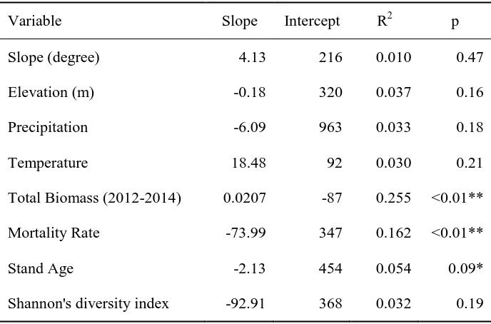
Type II (major axis) correlations between biomass C change and environmental factors.
Table 2.4 26
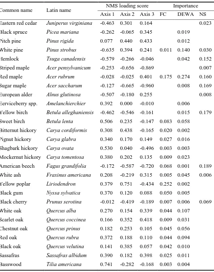
The loading scores of species on the three axes in the NMS analysis and their importance in each site.
Table 2.5 27
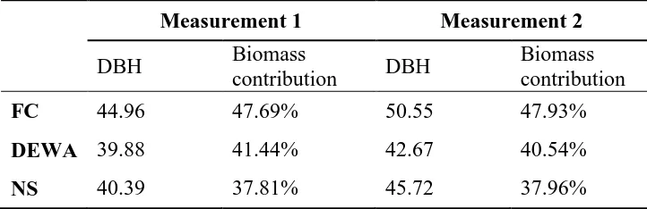
Average DBH of the 10% largest trees and their contribution to total live tree biomass in each site and measurement.
Table 3.1 55
Main problems associated with the soil core sampling method and their effect on soil properties. (“−”, no effect; “↑”, overestimate; “↓”, underestimate; “?”, uncertain)
Table 3.2 56
Environmental conditions in the three research sites in the Delaware River Basin. All data were extracted from a GIS data base and mean values for each site are shown. Annual temperature and precipitation are 30-year means from 1981-2010 (Thornton et al., 2014). Wet deposition is inorganic nitrogen deposition from 1983-2007 (Grimm, 2008).
Table 3.3 57
Soil C and N stocks and C/N sampled using soil core and soil pit methods in the three research sites in the Delaware River Basin. Sample size (n) represents number of plots sampled in each study site. In soil core method, organic layer was defined as a sum of Oi and Oe+Oa layers, and the C and N stocks measured in the two mineral layers (0-10 cm, and 10-20 cm) were summed together. Significant level of ANOVA testing for the effect of sites on C and C/N of each layer in the pit method are labeled as “*”, p<0.1; “**”, p<0.05. Significant differences (p< 0.05) among each pair of sites labeled by letter(s) next to the mean of each site.
xiv
Comparison of soil core and soil pit sampling methods: means, standard deviations and results of Wilcoxon Signed-rank Test for all soil properties in surface mineral soil layers (0-20 cm depth). Paired data from 57 plots using both soil sampling methods were used for the Wilcoxon Signed-rank Test.
Table 4.1 86
Environmental conditions in the three research sites in the Delaware River Basin. All data were extracted from the model input GIS database and mean values for each site are shown. Annual temperature and precipitation are 30-year means from 1981-2010 (Thornton et al., 2014). Wet deposition is inorganic N deposition from 1983-2007 (Grimm, 2008).
Table 4.2 87
Settings and input data used in PnET model simulation scenarios to test the effects of N deposition and elevated atmospheric CO2 concentrations.
Table 4.3 88
Parameter values used in the original and modified PnET model for the three major vegetation types present in the three study sites of the Delaware River Basin.
Table 4.4 89
Comparison of observed and model-predicted live forest biomass (Mg C ha-1) in each site in 2000 and 2010. The mean, standard deviation (SD) of spatial variations, and normalized root mean square error (NRMSE) for estimating predicted errors bythe original model and modified PnET-CN models are shown. The observed forest biomass data for 2000 were not used in the modification process, therefore could be considered as validation of model results.
Table 4.5 90
Model-predicted forest biomass (VegM, Mg C ha-1), soil C (SoilM, Mg C ha-1), net primary productivity (NPP, Mg C ha-1 yr-1) and net ecosystem productivity (NEP, Mg C ha-1 yr-1) in the three study sites of the Delaware River Basin, using the original model, modified model under full scenario, and modified model under CO2+N removed scenario. The effects of elevated CO2
and N deposition were calculated as the percentage change of each variable from the full scenario to the CO2+N removed scenario using the modified model. Negative effect values indicate that
elevated CO2 and N deposition resulted in increased values of the variables in the full scenario. Table 5.1 102
xv
LIST OF ILLUSTRATIONS
Figure 2.1 28
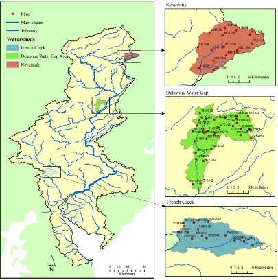
The hydrological boundary of the Delaware River Basin and the main stream and tributaries of the Delaware River. The three research areas of the current study are shown in different shading color. The red dots represent the locations of forest biomass plots.
Figure 2.2 29
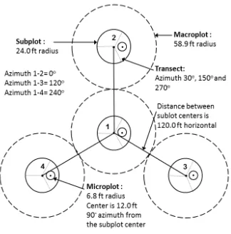
Plot design used for forest measurement (Revised from U.S. Department of Agriculture, Forest Service. (2002)). Trees within each subplot were measured. Sapling and seedlings were measured in microplots. Coarse and fine woody debris were measured on transects.
Figure 2.3 30
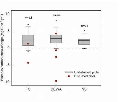
Biomass C stock changes in the three research sites and for all plots combined. Red dots represent the six disturbed plots. Boxes above the zero line represent increasing biomass C stock. Lines in the boxes show the median and the 25% and 75% quantiles, while bars outside the boxes show the 5% and 95% quantiles. Outliers are shown as black dots. FC: French Creek, DEWA: Delaware Water Gap, NS: Neversink.
Figure 2.4 31
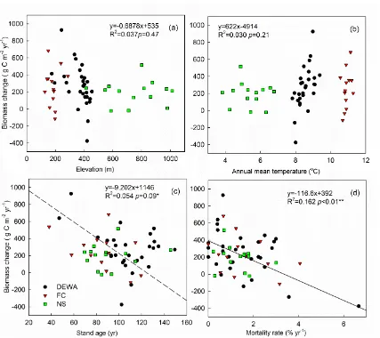
Relationship between biomass C stock change and environmental (a and b) and biotic (c and d) factors among all the undisturbed plots. Plots in the three sites are shown in different colors and shapes.
Figure 2.5 32
Live tree biomass C and mortality rates in different tree size classes. Live tree biomass C in the two measurements in (a) French Creek, (b) Delaware Water Gap, and (c) Neversink. Mortality rates (d) of the three research sites between the two measurements. The three sites are shown in different shades.
Figure 2.6 33
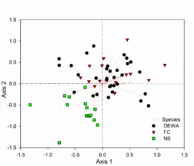
Results from the NMS for live trees in the second measurement (2012-2014). Points represent individual plots sampled and sites are represented by different colors. Arrows represent species. See Table 2.4 for the loading score of species.
Figure 2.7 34
Stem density and biomass C change in the fifteen most important species in the tree sites in the DRB forests: (a) French Creek (b) Delaware Water Gap (c) Neversink. The lengths of the bars represent the biomass C gain from recruitment and growth and biomass C loss from mortality. Data points on the left side of the zero line represent decrease in stem density or biomass C stocks, and on the right side of the zero line represent increase in stem density or biomass C stocks. See Table 2.4 for species Latin names.
Figure 2.8 35
xvi
Figure 3.1 59
The hydrological boundary of the Delaware River Basin and the main stream and tributaries of the Delaware River. The three research areas are shown in different shading color. The red dots represent the locations of soil sampling plots labeled by their plot ID.
Figure 3.2 60
Plot design of forest measurement and soil sampling (revised from U.S. Department of Agriculture, 2002). The red star represents the location of the quantitative soil pit. The FIA protocol uses ‘visit 1’, ‘visit 2’ (represent by blue dots) as the sampling locations in each of the sublot. The survey in 2012-2013 was the second measurement of these plots, so the ‘visit 2’ location of each subplot was selected for the soil core.
Figure 3.3 61
Correlations of (a) bulk density, (b) coarse fragment, (c) soil mass, (d) C concentration, (e) C stock, and (f) C/N mass ratio, measured by the soil core and soil pit methods. The 1:1 line and Type II (major axis) linear regression are shown, where slopes statistically different from 1 are denoted by †. The three sites are represented by different symbols (Neversink, ; Delaware Water Gap, ; French Creek, ). Vertical error bars represent the standard error among the cores (n = 3), versus only one pit (i.e., no horizontal error bars).
Figure 3.4 62
Relative contributions of variance and covariance of bulk density (BD), carbon concentration (%C), and soil volume (1-CF) to the variance of soil carbon stocks for the Neversink (NS), Delaware Water Gap (DEWA) and French Creek (FC) research sites, using the soil pit method (a) and the soil core method (b).
Figure 4.1 91
The hydrological boundary of the Delaware River Basin and the main stream and tributaries of the Delaware River. The three research areas of the current study are shown in different shading color. The red dots represent the locations of forest biomass plots.
Figure 4.2 92
Comparison between model-predicted and observed live forest biomass for the original (a) and modified (b) PnET model.
Figure 4.3 93
Spatial distributions of forest biomass, soil C, net primary productivity (NPP) and net ecosystem productivity (NEP) as simulated by the original and modified PnET models in the French Creek study site in the Delaware River Basin.
Figure 4.4 94-95
Spatial distributions of forest biomass, soil C, net primary productivity (NPP) and net ecosystem productivity (NEP) as simulated by the original and modified PnET models in the Delaware Water Gap study site in the Delaware River Basin.
xvii
Spatial distributions of forest biomass, soil C, net primary productivity (NPP) and net ecosystem productivity (NEP) as simulated by the original and modified PnET model in the Neversink study site of the Delaware River Basin.
Figure 4.6 97
1
CHAPTER 1: Introduction
1.1 Forest carbon stocks and the global carbon cycle
Forests are a vital component of terrestrial ecosystems, covering ~30% of the world’s land surface area (Bonan, 2008). Forests also play an important role in the global carbon cycle, accounting for ~45% of the carbon stored in the terrestrial biosphere (Dixon et al., 1994). Forest biomass and soil are the two largest carbon pools in the forested ecosystem. At the global scale, the estimated forest carbon stocks are 536 Pg C in biomass and 1104 Pg C in soil (Field and Raupach 2004). The annual change of carbon stock was 2941 Tg C yr-1 in biomass and 456 Tg C yr-1in soil during 2000-2007 (Pan et al., 2011a).
As the forest carbon stocks in biomass and soil have increased consistently in the past several decades, their potential to sequester atmospheric carbon dioxide (CO2) is considered a mitigation
strategy to reduce global warming (Luyssaert et al., 2007; Ciais et al., 2013). It was estimated that forest carbon stocks in the United States increased 239 Tg C yr-1 in 2000-2007, which is equivalent to ~10 % of domestic carbon emissions (Turner et al., 1995; Birdsey et al., 2006). The forest in the Northeast region is a net carbon sink of 21.0 Tg C yr-1, compensating for 7.6% of the region’s fossil fuel emissions in 2001-2005 (Lu et al., 2013).
1.2 Forest biomass carbon stock and its controlling factors
2
disturbances (such as fire and harvest), and historical land use change determine the current stand age and succession stage of the forest, which could be the main drivers of biomass dynamics at the landscape scale (Caspersen et al., 2000; Pregitzer and Euskirchen, 2004).
During the process of forest succession following a large scale disturbance, living tree biomass accumulates and stem density decreases. This is the self-thinning process caused by competition for resources such as light and nutrient (Coomes and Allen, 2007). Changes in forest composition accompany this pattern as the species with different life strategies come to dominate the forest sequentially. At the later stages of succession, the forest reaches a steady state in which the accumulation of biomass saturates at large scale (Odum, 1969; Franklin et al., 2002; Walker et al., 2010; Yang and Luo, 2011). Most of the forests in the northeastern U.S. are secondary forests recovering from agricultural land use. However, carbon accumulation in some northern hardwood forests has been halted due to the impact of emerging stresses such as invasive pests and climate change (Ross et al., 2004; van Doorn et al., 2011; Gunn et al., 2014). This emphasizes the need to understand the linkage between tree demographic change and biomass carbon sequestration at multiple scales.
Forest biomass can also be affected by global environmental change induced by human activity. Global climate change can shift the distribution of different forest types (Gonzalez et al., 2010), extend growing seasons and stimulate both photosynthesis and respiration in plants (Menzel and Fabian, 1999; Walther et al., 2002). Climate change may also alter the frequency and severity of natural disturbance such as fire and drought (Dale et al., 2001), leading to a drastic change in forest biomass. Increasing atmospheric CO2 concentration and atmospheric nitrogen deposition
3
forest. These factors interact with each other, creating the complex mosaic of forest biomass distribution at the landscape scale (Anderson-Teixeira et al., 2013).
1.3 Forest soil carbon stock and its controlling factors
4
1.4 Modeling forest carbon cycling at a regional scale
Ecological models have been widely used in studying forest carbon cycling and its feedback with climate change. Process-based models are a powerful approach to test our understanding of biogeochemical processes and to extrapolate ground survey data from limited plots to the landscape scale (Yan et al., 2011). In addition, the environmental changes stemming from human industrial and agriculture activities, such as climate change, nitrogen deposition, elevated atmospheric CO2, increasing natural disturbances and land use change, interact with each other
through a complex set of mechanisms and their long term effects on forest carbon cycling are difficult to test in controlled experiments (Ollinger et al., 2002). Process models provide a useful tool stimulating these effects on ecological process and analyzing the relative importance of each factor (Felzer, 2012).
The PnET-CN model (Aber and Federer, 1992; Aber and Driscoll, 1997) is a process-based ecosystem model that uses spatial information on vegetation, climate and soil to simulate the carbon, nitrogen and water dynamics of forest ecosystems in the northeastern United States. The model has been validated in various forest types (Goodale et al., 2002; Ollinger et al., 2002; Chen et al., 2004). Regional versions of the model based on geographic information systems (GIS) have been developed to extrapolate the simulation from the site to the regional level (Pan et al., 2004a; Pan et al., 2009). Applications of PnET models have provided important insights into the interactive effects of climate change, nitrogen deposition, increasing atmospheric CO2 and ozone,
5
1.5 The Delaware River Basin (DRB) and the DRB Collaborative Environmental
Monitoring and Research Initiative
The Delaware River Basin (DRB) is a ~33,000 km2 watershed with tributaries in Pennsylvania, New Jersey, New York, Delaware, and Maryland. About 7.5 million people live in the DRB. An additional 8 million people in New York City and northern New Jersey rely on surface water diverted from the basin for their water supply (Fischer et al. 2004). A humid continental climate prevails throughout the DRB. The average annual temperature is 9-12 °C and the total average annual precipitation is 1143 mm (Kauffman et al. 2008). The DRB is located in the ecozone of deciduous forests and is ecologically diverse, with five physiographic provinces and multiple species assemblages that represent most of the major eastern forest type group (Murdoch et al., 2008). In the upper Appalachian Plateaus province the major forest type is Maple-beech-birch forest. In the lower part of Appalachian, valley and ridge, and piedmont provinces, the most prevalent forest type is Oak-hickory and Oak chestnut. Oak-pine forests are seen in New Jersey and south part of Delaware (Zhu and Evans, 1994). Coniferous forests intersperse in the upper Delaware Basin are residuals of historical landscape changes or the adaptation to local edaphic conditions.
6
Appalachian Plateau province; the Delaware Water Gap Area (DEWA) with three small watersheds (Adams Creek, Dingman's Falls and Little Bushkill) lying in the central Appalachian Plateau Province, and the French Creek Watershed (FC) in the midbasin Piedmont province. The CEMRI project has produced a large amount of valuable data, which underpins this Ph.D. study.
1.6 General questions addressed in this dissertation
Utilizing the data collected during the DRB CEMRI and additional field investigations during 2012 to 2014, the research presented in this dissertation addresses the spatial and temporal trends in biomass and soil carbon stocks in the DRB forests. To define the scope and direction of the current work, the primary questions which correspond to the individual research chapters are:
Chapter 2:
Forest biomass carbon stocks were estimated based on field measurement campaigns in 2001-2003 and 2012-2013. The change of biomass carbon stock in the DRB forest during the recent decade was quantified by comparing the two measurements. The controlling factors of forest biomass carbon change were investigated and the impact of tree demographic change on biomass carbon change was examined.
Question 1: How did forest biomass carbon stocks in the DRB change in the past decade?
Question 2: Which factors drive spatial variation in forest biomass carbon stock change?
Chapter 3:
7
variables to the spatial variation of soil carbon and nitrogen stocks were examined to evaluate the accuracy of the FIA soil core sampling method.
Question: Does the standard FIA soil core sampling protocol adequately quantify carbon content in the soils of the DRB?
Chapter 4:
The PnET-CN model was localized and improved by using field measured parameters, calibration by observed biomass data and incorporating disturbance history information. The model was used to generate maps of biomass and soil carbon stocks, and forest productivity in the three study sites in the DRB. The individual and combined effects of nitrogen deposition and CO2
fertilization were evaluated by comparing model results using different scenarios.
Question 1: How are the forest carbon pools and fluxes spatially distributed in each sites?
8
CHAPTER 2
Decadal Change of Forest Biomass Carbon Stocks and Tree Demography
in the Delaware River Basin
This chapter has been submitted for publication as:
Xu B., Y. Pan, A.F. Plante, A.H. Johnson, J.A. Cole, and R.A. Birdsey. Decadal Change of Forest Biomass Carbon Stocks and Tree Demography in the Delaware River Basin. Forest Ecology and Management. submitted
Abstract
9
10
2.1. Introduction
As global forest C stocks have increased consistently in the past several decades, their potential to sequester additional atmospheric carbon dioxide (CO2) is considered a mitigation strategy to
reduce global warming (Luyssaert et al., 2007; Pan et al., 2011; Ciais et al., 2013). Quantifying forest biomass C stock change and identifying the factors causing changes are important to understand forest dynamics and its feedback with climate change, and to successfully implement forest carbon management strategies (Hyvonen et al., 2007; Bonan, 2008). However large uncertainty still exists as forest biomass is highly heterogeneous (both spatially and temporally), and its dynamics are determined by different factors at different scales (Birdsey et al., 2006; Pan et al., 2013).
It is widely accepted that seasonal weather and climate regulate short-term fluctuations of carbon uptake, while disturbance history and management control C stock change on decadal time scales (Barford et al., 2001; Williams et al., 2012). Climatic, topographic and geologic factors determine forest dynamics across a broader range of environmental conditions, while stand age and gap dynamics control biomass accumulation at smaller spatial scales (Brandeis et al., 2009; Yi et al., 2010). Living tree biomass is one of the largest and most active C pools in forest ecosystems (Woodbury et al., 2007), and its dynamics are driven by the balance among three forest demographic changes: growth, recruitment and mortality (including harvesting). Each of these demographic changes can vary with age and species (Vanderwel et al., 2013a; Rozendaal and Chazdon, 2015). Long-term, periodic biometric measurements provide a unique opportunity to not only investigate forest biomass C dynamics at the regional scale, but also link biomass C stock with demographic change (Curtis et al., 2002; Xu et al., 2014).
11
northern hardwood forests has been halted due to the impact of emerging stresses such as invasive pests, land use change and climate change (Brooks, 2003; Siccama et al., 2007; Duarte et al., 2013). Small scale disturbances such as invasive pests, disease and selective harvesting may affect species differently, and increase C turnover at regional scales (Makana et al., 2011). The Delaware River Basin (DRB), situated in the southern edge of the northern hardwood forest, features diverse forest types and land-use histories. Most of the forests in the DRB are secondary forests recovering from agricultural land use, with stand ages around 80-100 years. Demographic change of different species composition in the DRB during the recovery process may reflect the impact of vegetation dynamics on forest biomass C change (Xu et al., 2012). These forests are sensitive to the controlling factors defining forest dynamics; thus, quantifying the biomass C stock in DRB forests acts as the basis for regional C cycle assessment and is essential for effective forest C management.
12
2.2. Methods
2.2.1 Research area
The Delaware River is one of the major rivers in the mid-Atlantic region of the United States, draining an area of about 33,000 km2 in Pennsylvania, New Jersey, New York, Delaware, and Maryland. The Delaware River Basin is characterized by a humid continental climate, with mean annual temperature of 9-12 °C and mean annual precipitation of 1143 mm (Kauffman et al., 2008). The DRB is located in the eco-zone of deciduous forests and is ecologically diverse, comprised of five physiographic provinces and multiple species assemblages that represent most of the major eastern U.S. forest types (Murdoch et al., 2008).
Three areas in the DRB were selected as intensive monitoring and research sites for process-level studies in forested landscapes: the Neversink River Basin (NS) in the northern, mostly forested region of the Appalachian Plateau province; the Delaware Water Gap Area (DEWA) with three small watersheds (Adams Creek, Dingman's Falls and Little Bushkill) lying in the central Appalachian Plateau Province; and the French Creek Watershed (FC) in the midbasin Piedmont province (Fig 2.1).
13
2.2.2 Field measurements and biomass C calculations
The plot design and sampling method follow the forest inventory protocols in the two measurements, including additional variables that were specified for the intensive study sites (Fig 2.2; U.S. Department of Agriculture, 2014). Each plot has four round subplots, in total covering an area of 672.44 m2. Live and dead trees, stumps and residue materials were measured in each subplot. DBH, total and bole height, tree species, and status change (e.g., live versus dead) of each tree were recorded. A laser rangefinder was used to measure the tree and bole heights. Each subplot has one microplot (area: 13.49 m2) and three transects (length: 7.92 m). Live and dead sapling (1 inch < DBH < 5 inch), seedling (DBH < 1 inch), shrub and herb coverage were measured in the microplots. Coarse woody debris and fine woody debris were measured along the transects. Within each plot, two trees close to the subplots that represent the dominant species and growing condition of the forest stand were selected as site trees. The age of the site trees was measured by counting rings in a tree core. The stand ages of plots were determined as the mean age of the two site trees.
Field measurement data from the original 2001-2003 inventory were acquired from a USFS database generated by the CEMRI project (http://www.fs.fed.us/ne/global/research/drb/summary.html). Data from the two inventories were compiled into a single database for biomass C calculations. Cole et al. (2013) provides a detailed description of the database, which contains CEMRI project data on tree biomass.
14
biomass, and the general equations were used to calculate coarse roots biomass. The total biomass of each tree was the sum of above-ground biomass and coarse roots. Dead tree biomass was multiplied by a reduction factor according to their decade classes and species groups (Waddell, 2002) to subtract the biomass loss from decomposition. Biomass of coarse woody debris and fine woody debris were calculated using standard equations (Woodall and Williams, 2005). Stump biomass was calculated as coarse root biomass multiplied by the reduction factor according to the decade classes. A conversion factor of 0.5 was used to convert biomass to C stock. The biomass C change of each component was calculated as the difference of biomass C in the two measurements divided by the number of years between the two measurements in each of the plot.
2.2.3 Data analysis
All data of topographic and climatic factors were extracted from spatial data layers based on the coordinated of each plots. The elevation data was derived from Global Land Cover Characterization datasets (https://lta.cr.usgs.gov/GLCC). Annual temperature and precipitation are 30-year means from 1981-2010 (Thornton et al., 2014). Wet deposition is inorganic nitrogen deposition from 1983-2007 (Grimm, 2008). The mean values of each site are shown in Table 2.1.
15
Tree species richness (S), Shannon's diversity index (H), and evenness (EH) were calculated for
each plot using the live tree data in the second measurement to represent the species diversity at plot level. For each site, species importance values were determined as (relative live density + relative live basal area) ÷ 2 as described by (Forrester et al., 2003) for each species. The 15 most important species in each site were selected and their biomass C and density change was examined. Biomass C loss from mortality was calculated as the biomass C of trees that were live in the first measurement and died before the second measurement. Biomass C gain from recruitment was calculated as the biomass of new ingrowth trees in the second measurement. Biomass C gain from growth was calculated as the biomass increase for trees living in both of the two measurements.
Differences among the three sites in total biomass C and biomass C change were compared using one-way ANOVA. Type II (major axis) regression analysis was used to test correlations between biomass C stock changes and biotic (stand age, tree mortality rate, Shannon’s biodiversity index) and abiotic (slope, elevation, temperature, precipitation, and wet nitrogen deposition) factors in all plots combined to detect regional patterns.
16
2.3. Results
2.3.1 Forest biomass C stock change and its components
Among the 61 plots that were revisited in 2012-2013, six plots had visible disturbances in the past decade. The biomass C loss in the disturbed plots was up to 9.72 Mg C ha-1 yr-1 (Fig 2.3). In the remaining 55 undisturbed plots, the total biomass C stocks were 146.7 Mg C ha-1 in FC, 114.7 Mg C ha-1 in DEWA, and 159.3 Mg C ha- 1 in NS in the first measurement during 2001-2003 (Table 2.2). In the second measurement during 2012-2014 of the same 55 undisturbed plots, the total biomass C stocks were 172.1 Mg C ha-1 in FC, 142.2 Mg C ha-1 in DEWA, and 185.1 Mg C ha- 1 in NS. The forests in the most northern site (NS), with higher elevation, and greater precipitation and nitrogen deposition, had larger biomass C pool than the other sites. The net biomass C stock change between the two measurements was 2.52 Mg C ha-1 yr-1 in FC, 2.68 Mg C ha-1 yr-1 in DEWA, and 1.94 Mg C ha-1 yr-1 in NS. The mean biomass C stock change in all plots was 2.45 Mg C ha-1 yr-1. The undisturbed forests in the DRB were therefore a net carbon sink over the recent decade (i.e., the mean of each site was above the zero line in Fig 2.3). The total biomass C change did not differ among the three sites (p=0.76).
17
2.3.2 Controlling factors in biomass C change
For all undisturbed plots combined, the change in biomass C stock between the two measurements was poorly correlated with climatic and topographic factors, although demonstrating divided domains (Table 2.3, Fig 2.4). Stronger correlations were detected between biomass C change and biotic factors (Table 2.3, Fig 2.4). The change in biomass C increased significantly with total biomass in the second measurement (r = 0.505, p < 0.01), and with tree mortality rate between the two measurements (r = -0.403, p < 0.01). Biomass C change was negatively correlated with stand age (r = -0.232, p = 0.09). No significant correlation was detected between biomass C change and tree species diversity.
2.3.3 Forest demographic changes
Large trees (>35 cm DBH) made greater contributions to the living biomass, especially in FC where the largest size class (> 45 cm DBH) accounted for 37.8% of the total live tree biomass. Live tree biomass increased between the two measurements in all size classes, but the change in biomass was greater in large size classes than in small size classes (Fig 2.5a-c). Mortality rates were also greater in smaller size class (10-20 cm DBH, Fig 2.6d) compared to trees in the middle size class (20-35 cm DBH). High variability was observed in large size class mortality rates because there were few large trees (>35 cm DBH, Fig 2.5d).
18
DEWA was not significant on both of the axes (axis 1: p = 0.73, axis 2: p = 0.59). Forests in NS were dominated by maple-beech-birch forest, while in FC and DEWA consisted of tree species typical of a southern deciduous type of oak-hickory forest. The DEWA site, located between the other two sites from north to south, appears to be more of a transition zone for tree species (Table 2.4).
Over the past decade, in spite of reduced stem density, the biomass C stock increased in the 15 most important species in the DRB forest (Fig 2.7). Growth of existing trees accounted for most of the biomass C increase, while recruitment contributed little to total biomass C change. Conversely, mortality played an important role in counterbalancing growth and recruitment. Because of the high mortality rate, the living biomass of chestnut oak, white oak and black oak decreased in FC and DEWA. White pine, red oak and sweet birch increased in both biomass and stem density in the oak-hickory forests in DEWA. In the maple-beech-birch forests in NS, the stem density of American beech, and biomass C stock of yellow birch and hemlock increased dramatically.
2.4. Discussion
2.4.1 The large biomass C sink in the DRB forests
19
Doorn et al., 2011). The change in biomass C stock was also greater than the national average of biomass C stock change during 2000-2007 (Pan et al., 2011).
Forest biomass C stocks differed significantly among the three sites (Table 2.2). Larger potential biomass C stocks in the maple-beech-birch forest and fewer disturbances at high elevation may be responsible for the larger biomass C stock in the NS (Turner et al., 1995). For the two sites dominated by oak-hickory forest (i.e., FC and DEWA), FC had a larger biomass C stock but smaller biomass C change, suggesting that the plots in FC were in a later successional stage compared to the plots in DEWA. The greater contribution of biomass C from the largest size classes and the high mortality rate in smaller size classes in the FC (Fig 2.5a and d) also indicated forest maturity. Although the average stand age in FC was younger than in DEWA (Table 2.1), it is likely that the warmer climate and greater atmospheric N deposition has allowed the forest in FC to accumulate more biomass C in a shorter period of time, and the growth rate of biomass C might have started to decline earlier (Odum, 1960; Anderson-Teixeira et al., 2013). In contrast, biomass C stocks increased at a greater rate in DEWA because the forests were in a relatively earlier successional stage and have greater potential to sequester more biomass C in the future.
20
2.4.2 Environmental versus biotic factors in determining biomass C change
The observed lack of correlation with climatic and topographic factors for biomass C change is likely because the plot variation in forest biomass is much larger than the spatial variation in environmental factors (as illustrated by scattering in a wide range vertically, but clustering in a small range horizontally in Fig 2.4a and b). The environmental factors were not adequate to explain the variation in biomass C change within each site, while biological factors such as tree mortality rate and stand age appeared to be more important in determining variation in biomass C stock changes. Our results suggest that forest biomass C change at the regional scale was mostly driven by internal community-level processes such as competition and natural succession, more so than external environmental factors. This is consistent with other research about the controlling factors of forest dynamics (Kardol et al., 2010; Nowacki and Abrams, 2015; Zhang et al., 2015).
To explain the lack of correlation between environmental factors and biomass C change, two points need to be mentioned. First, this result does not mean that forest biomass C is unaffected by climate change in the DRB. The total biomass C change we reported is a combination of natural growth and enhancement by climate change (Caspersen et al., 2000), whose effects cannot be easily separated because we have only two measurements and one-time interval. Second, environmental factors may determine demographic change and disturbance regime, and therefore may have indirect impacts on biomass C change (Vanderwel et al., 2013b; Baez et al., 2015). However, these effects are not strong enough to be detected at such small spatial scales compared to the more dominant influence of plot dynamics. Long term observations at more sites are needed to address the interactions between factors.
21
because the range of stand ages in our DRB plots was relatively narrow, and the correlation was mostly driven by the three plots with the youngest stand ages. The observation that younger forests accumulated more biomass C than older forest over the past decade still indicated that most of the forests in the DRB had reached or passed the stage of maximum growth rate. While still accumulating C and thus acting as a sink, the rate at which C may be sequestered in the future may decrease as the age distribution shifts toward older stands in the DRB forest.
Although live biomass C loss from mortality could be preserved in the ecosystem as dead biomass for several decades, tree mortality rates still had a significant impact on biomass C change (Fig 2.4d). A larger proportion of the spatial variation in biomass C change can be explained by tree mortality rate, rather than the average tree growth rate (Table 2.3), indicating the importance of tree mortality in determining forest dynamics (Purves et al., 2008; Xu et al., 2012). It has been reported that tree mortality rates vary with climate, forest density, species and succession stage (Bell, 1997; Brown and Schroeder, 1999; Lutz and Halpern, 2006; Bond-Lamberty et al., 2014). In the following discussion, we therefore further examine tree mortality rates by size class and species, and their impacts on biomass C change.
2.4.3 Demographic changes in different size classes and species
22
they have better access to more resources such as light and water (Stephenson et al., 2014). The fact that large trees in the DRB forests are still growing rapidly indicated a large potential for biomass C increase in the future. In this study, most of the trees in the largest size class (50-70 cm DBH) are comparable to only the middle size class in the old-growth forest of the Mid-Atlantic (McGarvey et al., 2015). This comparison further suggests that the forests in the DRB are likely in a stage of middle succession, and could continue to be a carbon sink in the future, although C sequestration rate may decline.
The highest mortality rates were observed in the smallest tree size class (especially in FC, where the forest biomass largely consisted of the largest size class, Fig 2.5a and d), which can be explained by severe competition in the understory layer. Once individual tree height reaches the canopy height, growth is not limited by light and the mortality rate decreases (Bell, 1997; Miura et al., 2001). Our observations contrast with the pattern of mortality rate increasing with stem size as reported in an old-growth forest (Runkle, 2013). It is observed that as forests age, the peak of mortality biomass C loss shifts from young, small trees to large, dominant trees (Bond-Lamberty et al., 2014; Woods, 2014; Rozendaal and Chazdon, 2015). However, increased mortality rate in large trees was only present in DEWA, which has the largest sample size (number of trees = 953), and not in FC and NS, which both have a smaller number of trees in the largest size class.
23
regime (Canham et al., 2006; Kardol et al., 2010). Our results reflect the importance of species-specific disturbances such as non-native insects and diseases, which may threaten a single species or genus of trees (Lovett et al., 2002; Flower et al., 2013). These disturbances are gradually changing the species composition in the DRB forest and may have profound impacts on biomass C stock change by altering the demographic change in different tree species (Hicke et al., 2012; Fahey et al., 2013).
For example, in the oak-hickory forests in FC and DEWA, oak species (e.g. chestnut oak and black oak in FC, white oak and chestnut oak in DEWA) are declining in both stem density and biomass C stock. The possible reasons for oak decline include regional selective harvesting and defoliation induced by gypsy moth outbreaks, or infestation of sudden oak death (Murdoch et al.
2008).
In the maple-beech-birch forests in NS, the most dominant species, American beech, was affected by infestations of beech bark disease (Griffin et al., 2003; Lovett et al., 2013), causing the largest biomass C loss from mortality (mostly from the largest size class) and the largest biomass C gain from recruitment among all the species and sites. These results implied that the forests in the NS are in the aftermath phase of the disease, in which the disease may stimulate regeneration and change the forest structure (Houston, 1994; Forrester et al., 2003).
24
2.4.4 Implications for regional C cycle and forest management.
In this study, periodic long-term field measurements of forest biomass allowed the quantification of total biomass C stock change, addressing controlling factors of biomass C change and examining the impact of tree demographic change in the DRB forest. Our results provided important information for understanding forest recovery processes in major forest types of the northeastern U.S., and for improving ecological modeling and forest management at the regional scale. Our results showed that forest biomass in the DRB was a relatively large carbon sink over the past decade compared with other sites and the national average. It is likely that the DRB forest will continue to be a carbon sink in the coming decades, because the forest is in its middle rather than a late successional steady state (Odum, 1969). These results underscore the potential of regional forest carbon management for climate mitigation and can serve as the baseline information for evaluating biomass C sequestration in the DRB forest.
25
Table 2.1 Environmental conditions in the three research sites in the Delaware River Basin. All data were extracted from geographic information layers, and mean values for each site are shown. The elevation data was derived from Global Land Cover Characterization datasets (https://lta.cr.usgs.gov/GLCC). Annual temperature and precipitation are 30-year means from 1981-2010 (Thornton et al., 2014). Wet deposition is inorganic nitrogen deposition from 1983-2007 (Grimm, 2008).
Elevation (m)
Mean annual temperature
(ºC)
Mean annual precipitation
(mm)
Wet deposition (kg N ha-1)
Average stand Age
French
Creek (FC) 166 11.16 1171 6.55 85 Delaware
Water Gap (DEWA)
360 8.53 1219 6.33 107
Neversink
26
Table 2.2 Total biomass C stocks in the two measurements (unit: Mg C ha-1) and biomass C stock change in different components (unit: g C m-2 yr-1) in each site and in all plots combined. Standard deviations among plots are given in the parentheses. P values show the statistical significance of differences among sites in a one-way ANOVA.
FC (n=13)
DEWA (n=28)
NS (n=14)
Total
(
n=55)
P value
Total Biomass C ( Mg C ha
-1)
2001-2003
146.7 (50)
114.7 (39)
159.3 (37)
133.6 (45)
0.004**
2012-2014
172.1 (56)
142.3 (51)
185.1 (45)
160.2 (53)
0.017*
Biomass C change (g C m
-2yr
-1)
Live Tree
216.0 (255)
204.8 (262)
131.1 (117)
188.7 (231)
0.56
Dead Tree
57.3 (104)
20.2 (50)
-12.8 (113)
30.8 (106)
0.18
Sapling
-6.0 (21)
-6.2 (28)
18.4 (40)
0.2 (31)
0.036*
Seedling
1.2 (6)
10.2 (13)
2.1 (4)
6.0 (11)
0.010*
CWD
5.8 (45)
18.0 (63)
36.0 (37)
19.7 (54)
0.34
FWD
-15.5 (29)
5.5 (29)
1.2 (14)
-0.5 (27)
0.06
Stump
-8.2 (33)
-5.0 (37)
-6.0 (36)
0.80
Live
Biomass
212.1 (262)
210.7 (258)
151.2 (108)
195.9 (228)
0.84
Dead
Biomass
40.2 (131)
57.0 (122)
42.6 (104)
49.3 (118)
0.49
27
Table 2.3Type II (major axis) correlations between biomass C change and environmental factors.
28
Table 2.4 The loading scores of species on the three axes in the NMS analysis and their importance in each site.
Common name Latin name NMS loading score Importance Axis 1 Axis 2 Axis 3 FC DEWA NS Eastern red cedar Juniperus virginiana -0.463 0.301 0.164 0.023 Black spruce Picea mariana -0.262 -0.065 0.345 0.019
Pitch pine Pinus rigida 0.077 0.440 0.433 0.012
White pine Pinus strobus -0.635 0.394 0.241 0.011 0.140 0.030 Hemlock Tsuga canadensis -0.579 -0.266 -0.046 0.042 0.152 Striped maple Acer pensylvanicum -0.253 -0.656 -0.869 0.007 Red maple Acer rubrum -0.028 -0.025 0.401 0.175 0.274 0.160 Sugar maple Acer saccharum -0.127 -0.665 -0.960 0.008 0.169 European alder Alnus glutinosa -0.507 -0.180 0.255 0.008 Eerviceberry spp. Amelanchierchier
spp.
0.392 0.000 -0.010 0.006
Yellow birch Betula alleghaniensis -0.462 -0.546 -0.161 0.015 0.179 Sweet birch Betula lenta 0.506 0.235 -0.147 0.083 0.058
Bitternut hickory Carya cordiformis 0.308 0.438 -0.165 0.020 0.002 Pignut hickory Carya glabra 0.340 0.170 0.149 0.027 0.016 Shagbark hickory Carya ovata 0.530 0.040 -0.496 0.003 0.003 Mockernut hickory Carya tomentosa 0.380 0.202 0.135 0.009 0.023
American beech Fagus grandifolia -0.172 -0.587 -0.720 0.068 0.001 0.189 White ash Fraxinus americana 0.208 -0.219 0.315 0.005 0.045 0.006 Yellow poplar Liriodendron
tulipifera
0.379 0.751 -0.434 0.252 0.002 Black gum Nyssa sylvatica 0.370 0.120 0.088 0.050 0.005
Black cherry Prunus serotina -0.012 -0.419 -0.189 0.007 0.006 0.069 White oak Quercus alba 0.270 0.154 0.339 0.044 0.107
29
Table 2.5 Average DBH of the 10% largest trees and their contribution to total live tree biomass in each site and measurement.
Measurement 1
Measurement 2
DBH
Biomass
contribution
DBH
Biomass
contribution
FC
44.96
47.69%
50.55
47.93%
DEWA
39.88
41.44%
42.67
40.54%
30
31
32
33
34
35
36
37
38
CHAPTER 3:
Method comparison for forest soil carbon and nitrogen stocks in Delaware
River Basin
This chapter is in press as:
Xu B., Y. Pan, A.H. Johnson, and A.F. Plante. Method comparison for forest soil carbon and nitrogen stocks in Delaware River Basin. Soil Science Society of America Journal. DOI: 10.2136/sssaj2015.04.0167
Abstract:
39
accumulate greater uncertainty in spatial extrapolation to regional estimates of forest soil C and N stocks.
3.1. Introduction
Soils represent the largest carbon pool and a highly dynamic component of the terrestrial carbon cycle (Batjes, 1996). Quantifying forest soil C and N stocks is critical to understanding the ecological responses of forests to changes in climate, land use and management, and to improve global change models (Smith et al., 2012; Dib et al., 2014). However, the accuracy of forest soil C and N estimates is hampered by the difficulty in characterizing forest soil properties because forest soils can be rocky, inaccessible and spatially heterogeneous (Qureshi et al., 2012; Lark et al., 2014). In addition to this inherent variability, there is large uncertainty in forest soil C and N estimates associated with the soil sampling methods used (Gifford and Roderick, 2003; Jandl et al., 2014).
40
41
The quantitative soil pit method purportedly provides more accurate estimations of soil C and N stocks (Lyford, 1964). This method provides direct measurement of rock content and soil mass from a larger, more representative, volume of soil (Vadeboncoeur et al., 2012). There are fewer limitations for the location of a quantitative pit because it does not need to avoid the presence of rocks. In addition, deeper portions of the soil profile are more accessible in the pit method than the conventional coring method. Soil pit excavation was considered as the preferred soil sampling method in many studies evaluating methods in measurements of soil properties (e.g., Harrison et al., 2003; Kulmatiski et al., 2003; Levine et al., 2012). However, because the soil pit method is so labor-intensive, fewer pits than cores are likely to be sampled over the same landscape area and therefore spatial variability in soil properties may not be adequately characterized.
Estimation of soil C and N stocks requires resolving variables of BD, CF, soil C and N concentrations and soil depth. The choice of sampling method may bias each variable in different ways. In addition, variables may contribute differently to the spatial variation of soil C and N stocks in different sampling methods (Holmes et al., 2011; Schrumpf et al., 2011). Therefore, a comprehensive comparison between sampling methods, particularly the widely used soil core method and the standard quantitative soil pit method, considering all variables and their contributions to the spatial variation, is of fundamental importance for our prediction ability in estimating large-scale forest soil C and N stock changes.
42
ecological properties of the DRB and ongoing monitoring projects provided a good opportunity to explore the metrological uncertainty of soil C and N content at a regional scale.
In this study, the FIA standard soil core method and the quantitative soil pit method were used to estimate soil C and N stocks in three research sites in the DRB forest. The major goals of this study were to: 1) quantify soil C and N stocks to 20 cm using FIA soil core method, and to 40 cm using soil pit method in the DRB forest plots; 2) compare soil properties measured by soil core and soil pit methods in the 0-20 cm mineral soil layer; and, 3) compare the contribution of variables to the spatial variation of soil C and N stocks in the two sampling methods.
3.2. Methods
3.2.1. Study area and plot design
The Delaware River Basin is characterized by a humid continental climate, with mean annual temperature of 9-12 °C and mean annual precipitation of 1143 mm (Thornton et al., 2014). The DRB is located in the ecozone of deciduous forests and is ecologically diverse, comprised of five physiographic provinces and multiple species assemblages that represent most of the major eastern U.S. forest types (Murdoch et al., 2008).
43
In total, 60 forested plots were randomly located across the three research sites (14 in NS, 32 in DEWA and 14 in FC). The plots were established in 2001-2003 by the U.S. Forest Service and U.S. Geologic Survey, and designed according to FIA and Forest Health Management protocols (U.S. Department of Agriculture, 2004). Each plot had four round subplots, covering a total area of 672 m2 (Fig3.2). In each of the plots, three soil cores 20 cm) and one quantitative soil pit (0-40 cm) were sampled at systematically located positions as described below. If the locations for sampling landed on non-forested areas (e.g., road, water body, farmland, etc.), no sample was collected. All the soil samples in FC, DEWA and three plots in NS were collected in summer 2013, while the remaining eleven plots in NS were sampled in summer 2014.
3.2.2. Standard FIA soil core sampling method
The standard FIA soil core sampling protocol was used to collect soil core samples (U.S. Department of Agriculture, 2004). Core samples were collected 9.14 m away from the center of subplots 2, 3 and 4 (Fig 3.2). In 2001-2003, soil samples had been collected at the location of ‘visit 1’ in these DRB plots. So in this second measurement, the coring was located at ‘visit 2’ of each subplot, to avoid the disturbance of the previous survey. In the standard FIA protocol, only one mineral soil sample is collected at subplot 2, while in this study, mineral soil samples were collected in each of the 3 subplots (Fig 3.2) to get more representative samples (i.e., larger area) to compare with the soil pit method.
44
obstructed by a rock or large root, the actual depth of the two layers were recorded and the space beneath was assumed to be occupied by rocks. If the mineral soil horizons were shallower than 3 cm, no mineral soil sample was collected for that subplot, and samples from the remaining two subplots were used. Although they can be used to sample deeper soils, the coring was performed only to 20 cm to comply with FIA standard methods.
3.2.3. Quantitative soil pit sampling method
The middle point between the plot center and subplot 4 was selected as the location for the quantitative soil pit in each plot (Fig 3.2). If this location was not forested (e.g., located on agriculture land or on a road), or had a tree or rock outcrop within the sampling area, the same location in subplot 2 or subplot 3 was selected.
45
the pit, the portion of rocks that could not be submerged into the perlite was not placed back into the pit but was instead weighed. The volume of the rocks was then calculated using a standard rock density of 2.65 g cm-3 (Telford et al., 1990) and was subtracted from the volume of the perlite.
3.2.4. Soil C and N analyses and C and N stocks calculations
Organic layer samples were oven dried at 105 °C for more than 12 hours, then ground to < 2 mm. Mineral soil samples were air-dried and sieved through a 2-mm screen. Twenty mineral samples representing the two soil layers distributed among the three research sites and collected by both methods were oven dried, and a correction curve between air-dry and oven-dry soil weights was generated (oven-dry = 0.9845 × air-dry, R2=0.999). Oven-dry weights of the mineral samples were estimated using this curve. An aliquot from each sample was ground by mortar and pestle to pass a 250-µm sieve to increase sample homogeneity. Ground samples (e.g., 15 mg for mineral soil and 5 mg for organic soil) were analyzed for total C and N concentrations (g kg-1) using an ECS4010 Elemental Analyzer (Costech, Valencia, CA, USA). Approximately 11 % of the samples (n = 71) were measured twice to verify the precision of the C and N analyses. These analytical replicates showed a precision in line with instrumental error (i.e., coefficient of variance of ~5 % for both C and N). Soil survey data for these regions indicates a lack of carbonates and soil pH values of 4.0 to 7.5 (Soil Survey Staff, 2014). We therefore equated total C concentrations to organic C. C/N ratios were calculated as the mass ratio between C and N concentrations.