Copyright by author(s); CC-BY 1777 The Clute Institute
Spatial Structure Behind The Ripple Effect:
The Case Of Hong Kong
Kwok-Chiu Lam, Shanghai University of Finance and Economics, Shanghai, China
ABSTRACT
This paper aims to study the spatial structure of Hong Kong residential market using census data with the urban model, and examine more critically the ripple effect found by Lam (2015). Empirically, those irregularities observed can be explained rather satisfactorily following the lines of reasoning by Brueckner (2011). As for the aforesaid ripples, we demonstrate that the drift pattern no longer exists after introducing a structural breakpoint in End-2008. Instead, we contend that irrespective of house sizes, all price changes tend to originate from the New Territories. And we propose two theoretical explanations for it: internal migration and spatial coefficient heterogeneity.
Keywords: Spatial Structure; Urban Model; Ripple Effect; Hong Kong
1. INTRODUCTION
he property market of Hong Kong as a Special Administrative Region of China is a hot research topic. It catches wide global press attention not only for the territory’s high population density (Demographia, 2016a), but also for its severely unaffordable housing prices (Demographia, 2016b). Segregating its private residential market into segments pertaining to geographical area and class/size, Lam (2015) examines the intraclass ripple effects and contends that the origin of price change shifts in the southerly direction along the area continuum as the house size increases. Yet no convincing explanations have been put forth. In order to do so, prior understanding of the spatial pattern of Hong Kong is required. This study is to fulfil two purposes: (i) sheds new insights into the spatial structure of Hong Kong, and (ii) serves as a supplement to Lam (2015) with more elaboration of the aforesaid ripple effect. The rest of the paper is structured as follows: Section 2 introduces the theoretical groundwork of the monocentric urban model. Section 3 describes the data sources and methodology. Section 4 presents our empirical findings. Section 5 proposes some refinements to the urban model. Lastly, concluding remarks and limitations confronted in our study are laid out in section 6.
2. THEORETICAL GROUNDWORK OF THE URBAN MODEL
Maybe the spatial structure of a city cannot be better described without resorting to the monocentric urban model. The whole Hong Kong private residential market would be divided into segments for examination according to two dimensions: location and size. Our lines of thought behind this approach is not new. On the contrary, the model has been set forth decades ago. In its simplest form, the model postulates that business of all kinds can only be carried out in the central part (thus called the “central business district” or CBD) of a city. Under such circumstances, all factors of production and final products have to be transported to the CBD for its full functioning. It can readily be understood that higher transportation costs would be incurred as the location gets farther away from the CBD. Early in 1903, Richard M. Hurd has emphasized in his book Principles of City Land Values that urban land value depends on the distance toward the city center.1
As for residential location, Alonso (1964) pointed out that solely focusing on distance would remarkably raise the population density around the CBD, as residents could simply cut the sizes of their houses in an effort to minimize commuting costs in the form of reduced house price or rent. Thus, considering another dimension (that is, size)
1 The original sentence runs as: “Since value depends on economic rent, and rent on location, and location on convenience, and convenience on nearness, we may eliminate the intermediate steps and say that value depends on nearness,” cited by Alonso (1964), p.6.
Copyright by author(s); CC-BY 1778 The Clute Institute becomes necessary so as to make the model more adaptive. Using utility theory in microeconomics, he proposes that households makes their dwelling decisions based on location and size of the houses, subject to income budget constraints. The underlying idea is simple: other things equal, more distant houses are cheaper; the increases in commuting costs have to be “compensated” by larger sizes in effect that the occupants achieve the same utility level.
In a modern city, the concerns of households are usually not so simple. The demand side is normally characterized by heterogeneity and subtle segmentation, which are in turn determined by the socio-demographic characteristics of the community and a myriad of salient housing features shaping the preferences of homebuyers. Demographic factors like the ages of household members and life course events including childbirth, marital and employment status definitely come into play (Rabe and Taylor, 2010). The study results on European countries from Aassve, et al. (2013) confirm that, the age norms (deadlines) perceived suitable to leaving parental home vary with ages, educational levels, gender and most markedly, across countries. In Hong Kong, at least we learn that newly married young couples tend to reject co-residence with parents and prefer buying their own houses (Li, 2015). Still, it is likely for them to make their purchases in the neighborhood of parents to maintain close family ties. Young parents, on the other hand, might be more concerned with the physical attributes of dwelling, such as house size, number of rooms and presence of balcony, as well as environmental factors like the type of neighborhood and amenities (Anderson and West, 2006; Rabe and Taylor, 2010). It is a common belief that we like living with neighbors with similar characteristics. More specifically, racial composition in the surroundings may be a particular concern for locating a home (Kiel and Zabel, 2008). In fact, the distaste for income inequality in neighborhood is found to rise with income and fall with age and education level (Leung and Tsang, 2012). Li, et al. (2016) find that the air and noise pollutions in Hong Kong exert profound negative impacts upon the property value, particularly of those on lower floors. Some perceived environmental values are not directly measurable as such, but aesthetic or spiritual in nature.2 The view that amenities like better schools are valued by parents can be exemplified by a broad range of studies such as Fack and Grenet (2010) and Ferrari and Green (2013), noting that house prices are related negatively to travel distance to school but positively to school performance. Generally speaking, open space in the nearby neighborhood is found to have favorable influence on house prices (Anderson and West, 2006).3 Working groups might regard accessibility to workplaces or proximity to railway stations as very critical factors with a view to avoiding the nuisance of commuting (Choy, et al., 2007).4 That said, people in search for scenery and tranquility possibly prefer to reside in the suburbs. All these have highlighted the notion of spatial submarkets with regard to their non-reproducible characteristics. It is not our focus of this paper to disentangle the relative significance of all these features.5 Out of the endless list of attributes, we pick up two most crucial ones – location and size – as the bases to partition the residential market for further investigation, mainly due to availability of reliable data.6
3. DATA AND METHODOLOGY
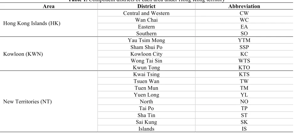
The land area of the Hong Kong territory is around 1,105.7 square kilometers (km2), as at End-2015. Spatially, the territory can be broken down (pointing northwards) into three areas: Hong Kong Island (HK), Kowloon (KWN) and the New Territories (NT). They approximately account for 7.3 percent, 4.24 percent and 88.46 percent of the total land area, respectively. Each of them is further subdivided into different (District Council) districts, with 18 districts in total. To save more space, a map is not inserted here. Interested readers may refer to the one ("GeoInfo Map" www2.map.gov.hk) drawn by Lands Department for the spatial delineation of all the constituent districts. Table 1 lists out the corresponding districts under each area. With respect to size, we would follow the usual practice by the Rating
2 As an example, some homebuyers are willing to pay premium on houses with good feng shui or located on “lucky number” floor. See Choy, et al. (2007) and Li, et al. (2016). For similar reasons, some might dislike the vicinity of funeral parlor.
3 More accurately, the value of open space hinges upon the dwelling’s location and neighborhood characteristics, dropping with the distance to the CBD and rising with the number of young children, population density, average household income, crime rates in the zone.
4 Railways are commonly favored by many Hongkongers because of punctuality and reliability. Railways here refer to Mass Transit Railway (Local line, East Rail line, Ma On Shan Rail line and West Rail line). According to Census and Statistics Department 2011 Population Census results, 34.4% of the working population rely on railways as their main mode of transport to place of work, compared to 32.4% on bus.
5 Overview of the most common housing attributes can be found in Boumeester (2011, Table 2.1) and Li, et al. (2016, Table 7.1).
Copyright by author(s); CC-BY 1779 The Clute Institute and Valuation Department (RVD), in that all private residential units are categorized according to the unit’s saleable area into: Class A – less than 40 m2 (A), Class B – between 40 m2 and 69.9 m2 (B), Class C – between 70 m2 and 99.9 m2 (C), Class D – between 100 m2 and 159.9 m2 (D), and Class E – 160 m2 or above (E). Hence, there are 15 segments altogether.
To investigate into the spatial pattern of Hong Kong residential market, we would mainly look at whether the regularities as specified by Brueckner (2011) can be observed. In the process, various demographic phenomena will be analyzed. All census data are deemed to be sourced from the Census and Statistics Department (CSD), unless otherwise stated. Notwithstanding our efforts to assemble as much data as we can, demographic data are relatively sparse and only compiled every (five) year(s) in Hong Kong. Better data can only be found starting from the 1980s or even 1990s. The approach we adopt here tends to be descriptive in nature. To further investigate the ripple spatial pattern unearthed by Lam (2015), we would employ the same data pool and denotations as his. To detect for structural change, we first regress territorywide real rental return (DLRRI_ALL) on real price return (DLRPI_ALL) using ordinary least squares equation and then perform “sequential l+1 breaks vs. l” and “global l breaks vs. none” multiple breakpoint testing methods over his sample period (1995M1 – 2014M12). Next, we would also deploy the same methodology, Granger-causality test with lag length p determined by Schwarz Bayesian information criterion (SIC) under a trivariate vector autoregressive model (VAR) at 10% significance level, to identify ripples in another sample period (1999M1 – 2014M12).7
Table 1. Component districts of each area under Hong Kong territory
Area District Abbreviation
Hong Kong Islands (HK)
Central and Western CW
Wan Chai WC
Eastern EA
Southern SO
Kowloon (KWN)
Yau Tsim Mong YTM
Sham Shui Po SSP
Kowloon City KC
Wong Tai Sin WTS
Kwun Tong KTO
New Territories (NT)
Kwai Tsing KTS
Tsuen Wan TW
Tuen Mun TM
Yuen Long YL
North NO
Tai Po TP
Sha Tin ST
Sai Kung SK
Islands IS
4. EMPIRICAL RESULTS
4.1 Spatial Structure
To portray the spatial pattern behind Hong Kong using the monocentric urban model, we initially posit that the central area is KWN and its CBD is situated at YTM. This is mainly because KWN occupies more amount (in m2) of private commercial (premises) in Hong Kong, relative to HK and NT (Panel A, Appendix 1). At the same time, YTM’s slice is exceptionally largest (47 percent) within that of KWN. Under such hypothesis, we herein discuss in the following several typical regularities as suggested by Brueckner (2011). As we will note, most of the irregularities observed, if any, can be explained more compellingly with refinements to the urban model.
Copyright by author(s); CC-BY 1780 The Clute Institute 4.1.1 Job Concentration
One manifestation of a typical CBD in a big city is high job concentration in the center due to agglomeration and scale economies. If the urban model is valid, the “places of work” should be more concentrated in KWN. Nonetheless, in Table 2, we see that the scenario of Hong Kong has called into question the accuracy of prediction from the model. Indeed, that feature is only more notable in 1996 in terms of percentage of our working population (excluding those who have no fixed work places or work on marine or outside Hong Kong).8 Yet as time goes by, the picture becomes more obscure and jobs opportunities appear to be more equally distributed amongst the three areas, even though KWN still supplies much more private commercial space than HK and NT.
Table 2. Working population by place of work: 1996 – 2011
1996 2001 2006 2011
Area No. % No. % No. % No. %
HK 910,777 32.05 929,574 31.31 938,047 30.88 989,763 31.14
KWN 1,043,844 36.74 1,033,855 34.82 1,055,449 34.74 1,099,452 34.59
NT 886,880 31.21 1,005,782 33.87 1,044,554 34.38 1,089,464 34.27
Overall 2,841,501 100.00 2,969,211 100.00 3,038,050 100.00 3,178,679 100.00
4.1.2 Residential Building Heights and Population Density
Presumably, as the location gets more outward from the CBD, (i) heights of residential buildings decrease and dwelling sizes increase and (ii) population density drops consequently. There are vast literatures on (ii), developing econometric models with increasing level of sophistication. Perhaps one of the earliest and most influential papers on the issue came from Colin Chark’s Urban Population Densities in 1951, recited in McDonald (1989), specifying that there existed a negative exponential function between gross population density and the distance to the CBD.9 While it is empirically infeasible to verify (i),10 it is easier to work on (ii) with census data. Population densities (number of persons per km2) of districts per area (1981 – 2011) are provided in Table 3.11 Apparently, KWN is much denser than HK, which is also much denser than NT, over the past three decades. A closer look at the district numbers reveals the same spatial tendency, especially in the 1980s. There is no doubt that the density of YTM is the highest being the CBD. Moving out into the boundaries in all directions, for example, YTM → SSP → ST → TW → YL → NO (northwards) or YTM → CW → SO (southwards), density decreases consistently. So the spatial population density has indeed behaved as predicted by the model.
Table 3. Population density by district per area (1981 – 2011)
Abbrev. 1981 1986 1991 1996 2001 2006 2011
HK
CW 23 448 20 854 20 479 20 755 21 137 20 102 20 057
WC 23 781 20 182 18 209 17 235 16 986 15 788 15 477
EA 27 150 27 387 30 316 31 735 33 147 31 664 31 686
SO 5 833 6 380 6 701 7 505 7 482 7 083 7 173
KWN
YTM 91 358 74 866 58 482 38 320 40 932 40 136 44 045
SSP 63 190 56 875 48 822 38 237 37 772 39 095 40 690
KC 54 207 47 156 41 759 38 553 38 059 36 178 37 660
WTS 53 947 46 940 41 331 42 331 47 810 45 540 45 181
(Table 3 continued on next page)
8 Of course, it is possible for a district to have big employment concentration in a particular industry. For instance, we might envision that jobs in the field of financing and insurance tend to be more concentrated in CW and WC of HK, where the headquarters are usually located. But concrete data of such kind seem unavailable officially. See also subsection 5.4.
9 Gross density refers to population per unit of total land; net density refers to that of residential land specifically (p. 364). Hong Kong data compiled by CSD belong to the former category.
10 Reference to Brueckner (2011; Chapter 3) can be sought for theoretical explanation on irregular building height pattern in a city. The fact is that, the contracting household size in Hong Kong has spurred the demand for smaller-sized units (Lam, 2016). More new dwellings are likely to be built in the new towns in suburbs, giving the illusion that house sizes decrease as distance from CBD rises.
Copyright by author(s); CC-BY 1781 The Clute Institute
(Table 3 continued)
Abbrev. 1981 1986 1991 1996 2001 2006 2011
KTO 55 260 60 826 52 562 53 081 49 861 52 123 55 204
NT
KTS 7 970 21 464 21 158 21 793 21 578 22 421 21 901
TW 4 159 4 581 4 502 4 566 4 679 4 918
TM 1 529 3 611 4 711 5 663 5 919 6 057 5 882
YL 1 397 1 545 1 664 2 465 3 242 3 858 4 178
NO 844 1 074 1 211 1 689 2 184 2 055 2 228
TP 551 1 033 1 496 2 103 2 287 2 156 2 181
ST 1 797 5 402 7 378 8 468 9 157 8 842 9 173
SK 339 365 1 026 1 542 2 535 3 135 3 368
IS 283 290 293 364 498 783 807
OVERALL 4 879 5 225 5 385 5 796 6 237 6 352 6 544
4.1.3 House Price and Rent
Another regularity implied from the simple urban model is that average purchase price or rental (in HKD) per m2 would fall moving away from the central zone, serving as compensation for the nuisance of commuting.12 To see whether such relationship really exists in Hong Kong, we collect quarterly data (1999Q1 – 2014Q4) from RVD ― (i) average house prices and (ii) average monthly rents ― for each class per m2 per area.13 The former (upper row) and the latter (lower row) have been plotted in Figure 1 for the ease of interarea comparison under different classes. It exhibits rather surprisingly (in particular, during the past 15 years) that the average price and rent of HK are always higher than that of KWN, which are in turn higher than that of NT. In other words, our diagrammatic analyses results have somehow belied the corollary of the urban model. Simply stated, as we move afar in the northerly direction into the suburbs (KWN → NT), house price and rentals indeed drop. Whereas, price and rentals rise unexpectedly moving southwards (KWN → HK).
Figure 1. Average price and monthly rent per m2 of all segments
A B C D E
0 20,000 40,000 60,000 80,000 100,000 120,000 140,000 199 9 200 0 200 1 200 2 200 3 200 4 200 5 200 6 200 7 200 8 200 9 201 0 201 1 201 2 201 3 201 4
HK KWN NT
0 20,000 40,000 60,000 80,000 100,000 120,000 140,000 1 99 9 2 00 0 2 00 1 2 00 2 2 00 3 2 00 4 2 00 5 2 00 6 2 00 7 2 00 8 2 00 9 2 01 0 2 01 1 2 01 2 2 01 3 2 01 4
HK KWN NT
20,000 40,000 60,000 80,000 100,000 120,000 140,000 160,000 180,000 1 99 9 2 00 0 2 00 1 2 00 2 2 00 3 2 00 4 2 00 5 2 00 6 2 00 7 2 00 8 2 00 9 2 01 0 2 01 1 2 01 2 2 01 3 2 01 4
HK KWN NT
0 40,000 80,000 120,000 160,000 200,000 199 9 200 0 200 1 200 2 200 3 200 4 200 5 200 6 200 7 200 8 200 9 201 0 201 1 201 2 201 3 201 4
HK KWN NT
0 50,000 100,000 150,000 200,000 250,000 300,000 350,000 400,000 1 99 9 2 00 0 2 00 1 2 00 2 2 00 3 2 00 4 2 00 5 2 00 6 2 00 7 2 00 8 2 00 9 2 01 0 2 01 1 2 01 2 2 01 3 2 01 4
HK KWN NT
80 120 160 200 240 280 320 360 400 440 199 9 200 0 200 1 200 2 200 3 200 4 200 5 200 6 200 7 200 8 200 9 201 0 201 1 201 2 201 3 201 4
HK KWN NT
80 120 160 200 240 280 320 360 400 199 9 200 0 200 1 200 2 200 3 200 4 200 5 200 6 200 7 200 8 200 9 201 0 201 1 201 2 201 3 201 4
HK KWN NT
50 100 150 200 250 300 350 400 450 199 9 200 0 200 1 200 2 200 3 200 4 200 5 200 6 200 7 200 8 200 9 201 0 201 1 201 2 201 3 201 4
HK KWN NT
120 160 200 240 280 320 360 400 440 199 9 200 0 200 1 200 2 200 3 200 4 200 5 200 6 200 7 200 8 200 9 201 0 201 1 201 2 201 3 201 4
HK KWN NT
120 160 200 240 280 320 360 400 440 480 520 199 9 200 0 200 1 200 2 200 3 200 4 200 5 200 6 200 7 200 8 200 9 201 0 201 1 201 2 201 3 201 4
HK KWN NT
4.2 Ripple Effects
Due to suspicion that structural break in the residential market might occur over the sample period (1995M1 – 2014M12)14, we run the aforementioned two ingenious breakpoint tests using EViews 8.1. Under both methods, default settings (maximum breaks = 5; trimming percentage = 15; significance level = 0.05) are kept and
12 Brueckner (2011; p.29) has used the term “compensating differential” to explain the concept that lower price per square foot is necessary in order to elicit people’s relocation into a disadvantageous/distant place.
13 In accordance with the interpretation of RVD, average prices are based on an analysis of transactions scrutinized by the Department for stamp duty purposes. Average rents are based on an analysis of rental information (exclusive of rates and management charges) recorded for fresh lettings effective in the month being analyzed.
Copyright by author(s); CC-BY 1782 The Clute Institute heterogeneous error distributions are allowed across breaks. As shown in Appendix 2 and 3, the outcomes signify rather unanimously that within the period, there is one determined break and the break date is estimated to be 2008M12.15 Hence, the output has reinforced our belief of a structural break in End-2008. Coincidentally, this was exactly the time when US Fed first launched its quantitative easing stimulatory monetary policy during the global financial crisis, in effect boosting asset prices with falling interest rates (Williams, 2011; Joyce, et al., 2012). We therefore disaggregate the original sample period into two subsets: 1999M1 – 2008M11, and 2008M12 – 2014M12 wherein the Granger-causality tests are carried out accordingly. Associated diagnostic statistics have been tabulated in Appendix 4 and 5, respectively.
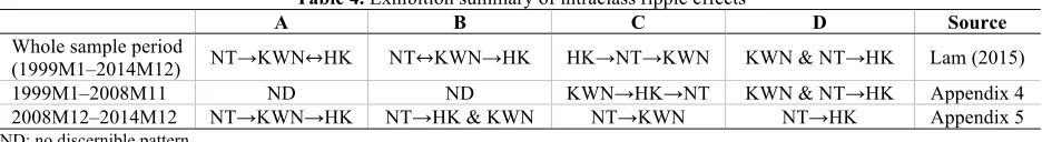
Unfortunately, the prior ripple effect documented by Lam (2015) has vanished during 1999M1 – 2008M11. Only one ripple is recognized in C, which is, KWN → HK → NT. Spanning 2008M12 – 2014M12, more discernible patterns are manifested: A (NT → KWN → HK); B (NT → HK and KWN); C (NT → KWN) and D (NT → HK). Our findings hereby indicate that irrespective of the class, all price changes actually originate from NT, with no shift at all. Possible reasons behind are deferred until Section 6. Hitherto all study results concerned can be summarized in Table 4 below.
Table 4. Exhibition summary of intraclass ripple effects
A B C D Source
Whole sample period
(1999M1–2014M12) NT→KWN↔HK NT↔KWN→HK HK→NT→KWN KWN & NT→HK Lam (2015)
1999M1–2008M11 ND ND KWN→HK→NT KWN & NT→HK Appendix 4
2008M12–2014M12 NT→KWN→HK NT→HK & KWN NT→KWN NT→HK Appendix 5
ND: no discernible pattern
5. REFINEMENTS TO URBAN MODEL
The notion of irregularities above causes no surprise, because the monocentric urban model in the present setting is clearly an over-simplification of Hong Kong. One reason we suggest for HK consistently high price and rent is that competition for land use in HK is more intense than in KWN and NT. We attempt to look for some other elucidations with the modifications laid down by Brueckner (2011), which have to take into account of unequal spatial income and time cost, internal migration, and scattered employment locations.
5.1 Competitive Land Use
Although the land area of HK is 70 percent larger than that of KWN, after excluding country parks in HK, the difference between the two becomes very modest.16 Relative to KWN, land in HK is more desperately in demand, not only for residential but also for office commercial purposes. Probably some light has been shed with our finding that (as at March 2016) out of the 50 constituent stocks of the Hang Seng Index, the principal business offices (within Hong Kong territory) of more than 40 are located in HK (almost exclusively in CW and WC along the coastal front of the Victoria Harbor). The truth is that, referring back to Panel B, Appendix 1, HK is the main source of private offices (of all grades) in the territory, accounting for more than half of the total supply.17 Therefore, it is more likely for larger proportion of land in HK to be reserved for (high-grade) office construction. The rationale is clear: land use is often determined by the highest bidder. This explains more plausibly why dwellings in HK often command the highest price and rents spatially.
5.2 Spatial Income and Time Cost
At the outset, one of the crucial implicit postulations underlying the simple urban model is that all households earn identical income. This occurs only very rarely. CSD has disseminated household median monthly income on district
15 The output results follow the EViews convention in defining break dates to be the first date of the subsequent regime after the break. Equivalently, 2008M11 is the last date of the preceding regime at which the break occurs. Refer to EViews (2014; p. 174 – 186) for interpretation of output results.
Copyright by author(s); CC-BY 1783 The Clute Institute basis at five-year interval before 2000 and annually hereafter. The incomes vary widely across districts over the course of time. In estimation of income per area, we compute the weighted average of the constituent district income, with weights equal to the number of households in the district divided by that in the area. The resultant spatial incomes over 1991 – 2014 are graphed in Figure 2. As shown, income in HK ranked the highest top while that in KWN and NT were almost identical (KWN = $9,323; NT = $9,281) in 1991. Nevertheless, starting from 1996, KWN has lagged behind of NT and their gap started to widen further since 2000.
The presence of unequal spatial income is more aligned with the real-world situation. Brueckner (2011) argues that higher income groups prefer more spacious and newer houses and do not mind commuting longer distance, so they are likely to move into the suburbs. The poor, by contrast, are inclined to stay in smaller-sized dwellings (despite higher per-square-foot price and rent) near the CBD wherein convenient public transit is often available. This ends up with the needy living near the center and the rich distant from it. To large extent, this is in line with the scenario in Hong Kong, where we have just demonstrated that household income in KWN has been overtaken by NT starting from mid-1990s. The result is that the wealthy move to either HK or NT, while the poor remain in KWN (especially in SSP).18
Another closely related concept derived from spatial income is the time cost borne by the affluent and the deprived. If we believe that the time of the rich is worth much more than that of the poor because of higher income earned by the former, the preceding implication from the urban model could be reversed, resulting in the former living near the center and the latter in the suburbs. This might partly explain why some of the well-offs live in HK (especially in CW and WC), just next to their office workplaces (but still not too far from YTM in KWN). This is possibly because their time is so precious! Therefore, once the fact that time costs differ among income groups is considered, the residing locations of them become indeterminate.
Figure 2. Household median monthly income by area (1991 – 2014)
5.3 Internal Migration
Population in absolute numbers and percentage of total population per area are illustrated under Figure 3. It substantiated strongly the tendency of internal migration from HK and KWN into NT. The population of KWN dropped rather considerably during the 1980s after which it becomes stabilized at around 2 million. Meanwhile, HK remains the least populous area of Hong Kong over the past 35 years. By contrast, we can see that the population in NT has nearly tripled over the same period and the migration trend will continue for the reasons that new town
18 SSP is just adjacent to YTM and remains the most deprived district in Hong Kong over the past 15 years.
9 000 14 000 19 000 24 000 29 000 34 000
1991 1993 1995 1997 1999 2001 2003 2005 2007 2009 2011 2013
HK
D
Copyright by author(s); CC-BY 1784 The Clute Institute developments are normally feasible only in NT and that the process has been facilitated by continual modernization of the transit railway systems (Li, et al., 2016).
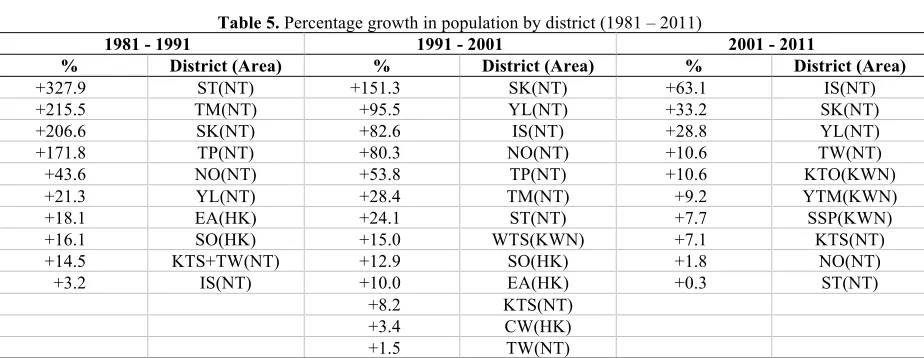
In Table 5, we have listed out all the district population growth rates (in descending order) over every decade between 1981 – 2011. In the 1980s, all NT districts have recorded positive growth. And the increases observed in ST, TM, SK and TP were explosive, largely thanks to the developments of new towns. Since the number of residents in HK has risen only mildly during the period, we can infer that there had been large internal migration from KWN (as demonstrated by its drastic drop as a whole) to the four districts in NT. In the following decade (1991 – 2001), the growth rates of seven out of the nine districts in NT have again ranked the very top, resulting in further 1-million surge in overall NT population. The growths in YL, IS and NO have been more impressive than in 1980s. In the meantime, modest growth and minimal decline have been recorded in HK and KWN, respectively. Hence, the prior trend of migration from KWN into NT just continued, but the pace has slowed down. Over the most recent decade (2001 – 2011), population in NT has expanded further by 0.35 million (mainly in IS, SK and YL). However, here exists a reverse direction, in that population in KWN has rebounded slightly (0.08 million), whereas those of HK has shrunk by a smaller amount (0.06 million). To sum up, over the past three decades, migration into NT is very evident. Equally noticeable is the tendency to reside outward into the edge of NT (for example, from ST and TM to YL, IS and NO) where land supply is more abundant. Even though the pace seems to have slowed down recently, NT is still believed to be the primary destination for in-migration as expanding railway network will make it more accessible and commuting costs lowered.
Figure 3. Population by area (1981 – 2011)
Table 5. Percentage growth in population by district (1981 – 2011)
1981 - 1991 1991 - 2001 2001 - 2011
% District (Area) % District (Area) % District (Area)
+327.9 ST(NT) +151.3 SK(NT) +63.1 IS(NT)
+215.5 TM(NT) +95.5 YL(NT) +33.2 SK(NT)
+206.6 SK(NT) +82.6 IS(NT) +28.8 YL(NT)
+171.8 TP(NT) +80.3 NO(NT) +10.6 TW(NT)
+43.6 NO(NT) +53.8 TP(NT) +10.6 KTO(KWN)
+21.3 YL(NT) +28.4 TM(NT) +9.2 YTM(KWN)
+18.1 EA(HK) +24.1 ST(NT) +7.7 SSP(KWN)
+16.1 SO(HK) +15.0 WTS(KWN) +7.1 KTS(NT)
+14.5 KTS+TW(NT) +12.9 SO(HK) +1.8 NO(NT)
+3.2 IS(NT) +10.0 EA(HK) +0.3 ST(NT)
+8.2 KTS(NT)
+3.4 CW(HK)
+1.5 TW(NT)
(Table 5 continued on next page)
0 1 000 2 000 3 000 4 000
1981 1986 1991 1996 2001 2006 2011
Po
pu
la
tio
n
('0
00
)
HK KWN NT
0 10 20 30 40 50 60
1981 1986 1991 1996 2001 2006 2011
Pe
rc
en
ta
ge
o
f
to
ta
l p
op
ul
at
io
n
Copyright by author(s); CC-BY 1785 The Clute Institute
(Table 5 continued)
1981 - 1991 1991 - 2001 2001 - 2011
% District (Area) % District (Area) % District (Area)
-7.5 KTO(KWN) -0.0 YTM(KWN) -0.3 TM(NT)
-10.8 CW(HK) -2.8 KTO(KWN) -1.0 KC(KWN)
-18.3 KC(KWN) -5.4 KC(KWN) -4.0 CW(HK)
-18.7 SSP(KWN) -7.1 SSP(KWN) -4.0 SO(HK)
-23.3 WTS(KWN) -7.3 WC(HK) -4.5 TP(NT)
-23.6 WC(HK) -4.6 EA(HK)
-33.6 YTM(KWN) -5.5 WTS(KWN)
-8.7 WC(HK)
5.4 Scattered Employment Opportunities
Heretofore we have hypothesized that there is only one CBD – YTM in KWN – in Hong Kong. However, as we have shown earlier, that the actual places of work are rather evenly dispersed among HK, KWN and NT. This mystery might be better unraveled by viewing Hong Kong as a “polycentric” city, wherein there is a secondary business district (SBD) in both HK and NT. Serving as employment subcenters, SBD furnishes extra job opportunities, possibly more associated with specific type of industries. After refining the model, an appealingly new direction is unfolded to understanding the spatial structure of the territory. Via comparing the relative size of stock in Appendix 1 of each kind among areas and districts, the major type of workplaces in different areas can be identified more specifically: commercial and retail premises [KWN] (Panel A), business offices [HK] (Panel B), and factories and industrial buildings [NT] (Panel C). At district level, YTM is the CBD in KWN as previously held, and, CW and KTS turn out to be the SBD of HK and NT respectively. Horizontal summation of all stock enables spatial comparison with the following results: 11,529,700 m2 (HK), 14,484,400 m2 (KWN) and 12,984,600 m2 (NT), or, in terms of percentage of total stock size in Hong Kong: 29.56 percent, 37.14 percent and 33.29 percent accordingly. Appreciably, the percentages resemble quite closely that of worksites of the working population in 2011 (Table 1).19
6. CONCLUSION
In this study, we heavily make use of census data (down to district level) to identify potential regular spatial patterns as recognized by Brueckner (2011) using the monocentric urban model in the context of Hong Kong. We find that such a simple model is incapable of elucidating fully the complicated setting of the modern city, and refinements are thus made to make it more adaptive. Moreover, we take one step forward after Lam (2015), by reckoning a structural break in 2008M11; after taking that into consideration, the shifting pattern of the ripple effect previously reported has simply collapsed. More strikingly, our results corroborate that NT leads the price changes of all classes since the structural change, without any drift.
Two articles from Meen (1999; 2001, Chapter 4) have distinguished several contributory factors to the formation of such spatial price patterns, two of which are especially relevant and deserve more discussion here: migration and spatial coefficient heterogeneity. The prolonged migration inflow into NT over the past three decades probably have attracted some of the rich, as reflected by its highest income growth between 2000 – 2014 [33.49 percent (HK), 31.57 percent (KWN), and 40.46 percent (NT)]. Its prices might be anticipated to be bidden up by largest extent. Yet we observe just the opposite.20 This surely shows the insufficiency of the explanation; as our recognition of ripples is only confined to 2008M12 – 2014M12. The second factor has underscored the importance of differing price responsiveness due to underlying structural differences in segments. For example, Li (2014, Chapter 5) finds stronger relationships between GDP and prices of larger-sized units. Lam (2016) not only acknowledges similar finding but also establishes
19 It can be argued that more accurate estimation of relative “workplaces” should be done by subtracting the corresponding vacant amount from stock. For simplicity, they are neglected in Appendix 1.
Copyright by author(s); CC-BY 1786 The Clute Institute that NT price is most sensitive to interest rate variations, relative to other areas. This fits in the episode that interest rates drop from End-2008 onwards, thus pushing up NT prices by greatest scale (170.69 percent).
Our evidence thus far is by no means conclusive. Neither do we think the above two explanations could explain perfectly the ripple effects. Rather, our paper attempts to, via discussion of the spatial pattern of Hong Kong, underline the socio-economic elements while analyzing our residential market, amid the main constraint of spatial demographic data shortage.
ACKNOWLEDGEMENTS
I feel greatly indebted to Prof. Ping Zou of Shanghai University of Finance and Economics for his forbearance in providing insightful comments and relentless support throughout the whole course of this research. Special thanks are also due to other faculty members at the School of Finance of the University for overall guidance. The usual disclaimer applies.
AUTHOR BIOGRAPHY
Kwok-Chiu Lam is a Teaching Fellow at School of Accounting and Finance, Hong Kong Polytechnic University, Hong Kong and also a PhD candidate at School of Finance, Shanghai University of Finance and Economics, Shanghai, China. Academic & professional qualifications: BBA (HKUST), MSc (CUHK), CFA, CFPCM, FRM. Research interest: investments, real estate finance and financial planning. Email: [email protected]
REFERENCES
Aassve, A., Arpino, B., & Billari, F. C. (2013). Age norms on leaving home: multilevel evidence from the European Social
Survey. Environment and Planning A, 45(2), 383-401.
Alonso, W. (1964). Location and land use: toward a general theory of land rent. Cambridge: Harvard University Press.
Anderson, S. T., & West, S. E. (2006). Open space, residential property values, and spatial context. Regional Science and Urban
Economics, 36(6), 773-789.
Boumeester, H. J. F. M. (2011). Traditional housing demand research. In S. J. T. Jansen, H. C. C. H. Coolen & R. W. Goetgeluk
(Eds.), The measurement and analysis of housing preference and choice, 27-55. Dordrecht/ Heidelberg/ London/ New
York: Springer.
Brueckner, J. K. (2011). Lectures on urban economics. Cambridge: MIT Press.
Choy, L. H. T., Mak, S. W. K., & Ho, W. K. O. (2007). Modeling Hong Kong real estate prices. Journal of Housing and the Built
Environment, 22(4), 359-368.
Demographia (2016a). Demographia world urban areas – 12th annual edition: 2016:04. Available at:
http://www.demographia.com/db-worldua.pdf
Demographia, (2016b). 12th annual demographia international housing affordability survey: 2016. Available at:
www.demographia.com/dhi.pdf
EViews (2014). EViews 8.1 User’s Guide II, IHS, Global Inc., Irvine CA, USA.
Fack, G. & Grenet, J. (2010). When do better schools raise housing prices? Evidence from Paris public and private schools.
Journal of Public Economics, 94(1-2), 59-77.
Ferrari, E., & Green, M. A. (2013). Travel to school and housing markets: a case study of Sheffield, England. Environment and
Planning A, 45(11), 2771-2788.
Joyce, M,. Miles, D., Scott, A., & Vayanos, D. (2012). Quantitative easing and unconventional monetary policy – an
introduction. The Economic Journal, 122(564), F271-F288.
Kiel, K. A., & Zabel, J. E. (2008). Location, location, location: the 3L approach to house price determination. Journal of Housing
Economics, 17(2), 175-190.
Lam, K.-C. (2015). Testing the present value model and domino (ripple) effects for Hong Kong private residential housing
prices. International Journal of Financial Research, 6(4), 22-35.
Lam, K.-C. (2016). The responsiveness of Hong Kong private residential housing prices. International Journal of Economics and
Financial Issues, 6(1), 26-36.
Leung, T. C., & Tsang, K. P. (2012). Love thy neighbor: income distribution and housing preferences. Journal of Housing
Economics, 21(4), 322-335.
Li, R. Y. M. (2014). Law, economics and finance of the real estate market – a perspective of Hong Kong and Singapore.
Copyright by author(s); CC-BY 1787 The Clute Institute
Li, R. Y. M. (2015). Generation X and Y’s demand for homeownership in Hong Kong. Pacific Rim Property Research Journal,
21(1), 15-36.
Li, R. Y. M., Chau, K. W., Law, C. Y., & Leung, T. H. (2016). Superstition and Hong Kong housing prices. In R. Y. M. Li & K.
W. Chau (Eds.), Econometric analyses of international housing markets, 92-115. New York: Routledge.
McDonald, J. F. (1989). Econometric studies of urban population density: a survey. Journal of Urban Economics, 26(3),
361-385.
Meen, G. P. (1999). Regional house prices and the ripple effect: a new interpretation. Housing Studies, 14(6), 733-753.
Meen, G. P. (2001). Modelling spatial housing markets: theory, analysis and policy. Boston/ Dordrecht/ London: Kluwer
Academic Publishers.
Rabe, B., & Taylor, M. (2010). Residential mobility, quality of neighbourhood and life course events. Journal of the Royal
Statistical Society, 173(3), 531-555.
Copyright by author(s); CC-BY 1788 The Clute Institute APPENDICES
Appendix 1. Stock (in m2) of private commercial, offices, and flatted factories at End-2014
Panel A: Private commercial
Panel B: Private offices
Panel C: Private flatted
factories
Abbrev. Total Grade A Grade B Grade C Total Total
HK
CW 1 125 300 1 904 800 771 400 577 500 3 253 700 66 900
WC 1 083 000 908 400 571 000 306 000 1 785 400 0
EA 765 200 740 000 201 900 79 800 1 021 700 1 254 800
SO 254 200 147 000 48 900 10 500 206 400 713 100
3 227 700 3 700 200 1 593 200 973 800 6 267 200 2 034 800
KWN
YTM 2 084 500 1 141 500 617 500 411 200 2 170 200 306 500
SSP 702 900 178 700 55 900 39 200 273 800 1 038 100
KC 712 000 107 300 49 200 20 400 176 900 850 500
WTS 320 000 0 45 700 1 200 46 900 763 300
KTO 629 200 1 152 500 72 900 12 500 1 237 900 3 171 700
4 448 600 2 580 000 841 200 484 500 3 905 700 6 130 100
NT
KTS 347 200 149 100 11 500 2 000 162 600 3 296 400
TW 499 000 114 600 10 300 800 125 700 2 321 400
TM 414 300 32 700 0 8 500 41 200 1 476 300
YL 468 400 9 200 9 800 19 000 38 000 203 400
NO 229 800 26 900 3 300 500 30 700 286 600
TP 232 000 0 5 200 1 200 6 400 151 900
ST 462 600 309 100 16 000 0 325 100 1 110 000
SK 290 300 9 000 0 0 9 000 9 000
IS 297 300 130 200 18 900 0 149 100 900
3 240 900 780 800 75 000 32 000 887 800 8 855 900
OVERALL 10 917 200 7 061 000 2 509 400 1 490 300 11 060 700 17 020 800
Copyright by author(s); CC-BY 1789 The Clute Institute
Appendix 2. “Sequential L+1 breaks vs. L” multiple breakpoint testing approach
Bai-Perron tests of L+1 vs. L sequentially determined breaks
Sequential F-statistic determined breaks: 1
Scaled Critical
Break Test F-statistic F-statistic Value**
0 vs. 1 * 10.96875 21.93750 11.47
1 vs. 2 4.384227 8.768455 12.95
Break dates:
Sequential Repartition
1 2008M12 2008M12
Copyright by author(s); CC-BY 1790 The Clute Institute
Appendix 3. “Global L breaks vs none” multiple breakpoint testing approach
Bai-Perron tests of 1 to M globally determined breaks
Sequential F-statistic determined breaks: 5
Significant F-statistic largest breaks: 5
UDmax determined breaks: 1
WDmax determined breaks: 1
Scaled Weighted Critical
Breaks F-statistic F-statistic F-statistic Value
1 * 10.96875 21.93750 21.93750 11.47
2 * 7.760468 15.52094 18.25899 9.75
3 * 5.860540 11.72108 16.08144 8.36
4 * 6.111012 12.22202 19.49744 7.19
5 * 5.163969 10.32794 20.24982 5.85
UDMax statistic* 21.93750 UDMax critical value** 11.70
WDMax statistic* 21.93750 WDMax critical value** 12.81
Estimated break dates: 1: 2008M12
2: 1998M04, 2008M12
3: 1998M04, 2001M11, 2008M12
4: 1998M04, 2001M11, 2005M04, 2008M12
5: 1998M04, 2001M11, 2005M04, 2008M12, 2011M12
Copyright by author(s); CC-BY 1791 The Clute Institute
Appendix 4. Pairwise Granger-causality test statistics on intraclass ripple effects (1999M1 – 2008M11)
Trivariate
VAR Lag p Null Hypothesis F-Statistic Probability Causality*
1 DLKWN_A_RP does not Granger Cause DLHK_A_RP DLHK_A_RP does not Granger Cause DLKWN_A_RP 12.3515 2.38599 0.1252 0.0006 HK → KWN
1 DLNT_A_RP does not Granger Cause DLHK_A_RP DLHK_A_RP does not Granger Cause DLNT_A_RP 9.26647 2.54637 0.0029 0.1133 NT → HK
1 DLNT_A_RP does not Granger Cause DLKWN_A_RP 22.2822 7×10
-6
KWN ↔ NT
DLKWN_A_RP does not Granger Cause DLNT_A_RP 3.45681 0.0656
1 DLKWN_B_RP does not Granger Cause DLHK_B_RP DLHK_B_RP does not Granger Cause DLKWN_B_RP 20.7774 0.28789 10.5926 ×10⁻⁵ KWN → HK
1 DLNT_B_RP does not Granger Cause DLHK_B_RP DHK_B_RP does not Granger Cause DLNT_B_RP 4.80264 6.17896 0.0304 0.0144 NT ↔ HK
1 DLNT_B_RP does not Granger Cause DLKWN_B_RP 2.91412 0.0905 NT ↔ KWN
DKWN_B_RP does not Granger Cause DLNT_B_RP 9.04923 0.0032
1 DLKWN_C_RP does not Granger Cause DLHK_C_RP DHK_C_RP does not Granger Cause DLKWN_C_RP 3.75011 1.82382 0.0553 0.1795 KWN → HK
1 DLNT_C_RP does not Granger Cause DLHK_C_RP DHK_C_RP does not Granger Cause DLNT_C_RP 0.78844 8.51668 0.3764 0.0042 HK → NT
1 DLNT_C_RP does not Granger Cause DLKWN_C_RP DKWN_C_RP does not Granger Cause DLNT_C_RP 0.90568 3.64107 0.3433 0.0589 KWN → NT
1 DLKWN_D_RP does not Granger Cause DLHK_D_RP DLHK_D_RP does not Granger Cause DLKWN_D_RP 5.59832 1.15275 0.0197 0.2852 KWN → HK
1 DLNT_D_RP does not Granger Cause DLHK_D_RP DLHK_D_RP does not Granger Cause DLNT_D_RP 3.69822 1.99024 0.0570 0.1610 NT → HK
1 DLNT_D_RP does not Granger Cause DLKWN_D_RP 0.45332 0.5021 n/a
DLKWN_D_RP does not Granger Cause DLNT_D_RP 0.11067 0.7400
Copyright by author(s); CC-BY 1792 The Clute Institute
Appendix 5. Pairwise Granger-causality test statistics on intraclass ripple effects (2008M12 – 2014M12)
Trivariate
VAR Lag p Null Hypothesis F-Statistic Probability Causality*
1 DLKWN_A_RP does not Granger Cause DLHK_A_RP DLHK_A_RP does not Granger Cause DLKWN_A_RP 10.1903 0.15113 0.0021 0.6986 KWN → HK
1 DLNT_A_RP does not Granger Cause DLHK_A_RP DLHK_A_RP does not Granger Cause DLNT_A_RP 8.65729 0.94996 0.0044 0.3331 NT → HK
1 DLNT_A_RP does not Granger Cause DLKWN_A_RP DLKWN_A_RP does not Granger Cause DLNT_A_RP 6.77046 0.74672 0.0113 0.3905 NT → KWN
1 DLKWN_B_RP does not Granger Cause DLHK_B_RP DLHK_B_RP does not Granger Cause DLKWN_B_RP 2.00460 0.23077 0.1613 0.6324 n/a
1 DLNT_B_RP does not Granger Cause DLHK_B_RP DHK_B_RP does not Granger Cause DLNT_B_RP 9.20854 1.43981 0.0034 0.2342 NT → HK
1 DLNT_B_RP does not Granger Cause DLKWN_B_RP 7.64320 0.0073 NT → KWN
DKWN_B_RP does not Granger Cause DLNT_B_RP 1.43431 0.2351
1 DLKWN_C_RP does not Granger Cause DLHK_C_RP DHK_C_RP does not Granger Cause DLKWN_C_RP 0.08451 2.57134 0.7721 0.1133 n/a
1 DLNT_C_RP does not Granger Cause DLHK_C_RP DHK_C_RP does not Granger Cause DLNT_C_RP 0.88706 0.48158 0.3495 0.4900 n/a
1 DLNT_C_RP does not Granger Cause DLKWN_C_RP DKWN_C_RP does not Granger Cause DLNT_C_RP 3.59609 1.97104 0.0620 0.1648 NT → KWN
1 DLKWN_D_RP does not Granger Cause DLHK_D_RP DLHK_D_RP does not Granger Cause DLKWN_D_RP 0.33644 0.93435 0.5638 0.3371 n/a
1 DLNT_D_RP does not Granger Cause DLHK_D_RP DLHK_D_RP does not Granger Cause DLNT_D_RP 3.19022 1.94249 0.0784 0.1678 NT → HK
1 DLNT_D_RP does not Granger Cause DLKWN_D_RP 0.98711 0.3239 n/a
DLKWN_D_RP does not Granger Cause DLNT_D_RP 0.12885 0.7207