University of Pennsylvania
ScholarlyCommons
Publicly Accessible Penn Dissertations
2017
Essays On Social Norms
Nicholas Janetos
University of Pennsylvania, njanetos@econ.upenn.edu
Follow this and additional works at:https://repository.upenn.edu/edissertations
Part of theEconomics Commons
This paper is posted at ScholarlyCommons.https://repository.upenn.edu/edissertations/2358 For more information, please contactrepository@pobox.upenn.edu.
Recommended Citation
Janetos, Nicholas, "Essays On Social Norms" (2017).Publicly Accessible Penn Dissertations. 2358.
Essays On Social Norms
Abstract
I study equilibrium behavior in games for which players have some preference for appearing to be well-informed. In chapter one, I study the effect of such preferences in a dynamic game where players have preferences for appearing to be well-informed about the actions of past players. I find that such games display cyclical behavior, which I interpret as a model of `fads'. I show that the speed of the fads is driven by the information available to less well-informed players. In chapter two, I study the effect of such preferences in a static game of voting with many players. Prior work studies voting games in which player's preferences are determined only by some disutility of voting, as well as some concern for swaying the outcome of the election to one's favored candidate. This literature finds that, in equilibrium, a vanishingly small percentage of the population votes, since the chance of swaying the election disappears as more players vote, while the cost of voting remains high for all. I introduce uncertainty about the quality of the candidates, as well as a preference for appearing to be well-informed about the candidates. I find that high levels of voter turnout are supported in equilibrium even when the number of players in the game is large. This resolves the empirical puzzle of why the chance of swaying the election should matter, given that it is very small.
Degree Type Dissertation
Degree Name
Doctor of Philosophy (PhD)
Graduate Group Economics
First Advisor Steven Matthews
ESSAYS IN SOCIAL NORMS
Nicholas Janetos
A DISSERTATION
in
Economics
Presented to the Faculties of the University of Pennsylvania in Partial
Fulfillment of the Requirements for the Degree of Doctor of Philosophy
2017
Steven Matthews, Professor of Economics
Supervisor of Dissertation
Jesus Fernandez-Villaverde, Professor of Economics
Graduate Group Chairperson
Dissertation Committee
Steven Matthews, Professor of Economics
ESSAYS IN SOCIAL NORMS
© Copyright 2017
Nicholas Janetos
This work is licensed under the
Attribution-NonCommercial-ShareAlike 4.0 International
License. To view a copy of
r
To my parents, who gifted me intellectual
Acknowledgments
I would like to thank the friends, family, teachers, and colleagues who supported me during
my graduate career.
In particular, I thank my colleagues Selman Erol, Dan Hauser, Ami Ko, Yunan Li, and
Laura Liu, for much fruitful discussion and feedback. I especially thank my co-author, Jan
Tilly, for his endless enthusiasm and inventiveness.
I thank the faculty at the University of Pennsylvania for fostering an atmosphere of
in-tellectual pursuit and excitement. In particular, I thank Aislinn Bohren, David Dillenberger,
Sangmok Lee, George Mailath, Mallesh Pai, Andrew Postlewaite, Alvaro Sandroni, Rakesh
Vohra, and Yuichi Yamamoto for their time and efforts. I would especially like to thank my
advisor, Steven Matthews, whose energy and dedication has made me a better researcher
and writer.
Nicholas Janetos
Philadelphia, PA
ABSTRACT
ESSAYS IN SOCIAL NORMS
Nicholas Janetos
Steven Matthews
My dissertation studies equilibrium behavior in games for which players have some
pref-erence for appearing to be well-informed. In chapter one, I study the effect of such
prefer-ences in a dynamic game where players have preferprefer-ences for appearing to be well-informed
about the actions of past players. In the main result, I find that such games display cyclical
behavior, which I interpret as a model of ‘fads’. I show that the speed of the fads is driven
by the information available to less well-informed players. In chapter two, I study the effect
of such preferences in a static game of voting with many players. Prior work studies voting
games in which player’s preferences are determined only by some disutility of voting, as well
as some concern for swaying the outcome of the election to one’s favored candidate. This
literature finds that, in equilibrium, a vanishingly small percentage of the population votes,
since the chance of swaying the election disappears as more players vote, while the cost of
voting remains high for all. I introduce uncertainty about the quality of the candidates, as
well as a preference for appearing to be well-informed about the candidates. I find that high
levels of voter turnout are supported in equilibrium even when the number of players in the
game is large. This resolves the empirical puzzle of why the chance of swaying the election
Contents
List of Figures viii
Introduction 1
1 Fads and imperfect information 5
1.1 Introduction . . . 5
1.1.1 Previous literature . . . 10
1.2 Illustrative example . . . 13
1.3 Static stage game. . . 21
1.3.1 Equilibria of the stage game . . . 23
1.4 Dynamic game . . . 31
1.4.1 Equilibria of the dynamic game . . . 38
1.4.2 Instrumental preferences for conformity . . . 40
1.5 Matching game application . . . 43
1.5.1 Comparative statics . . . 50
1.6 Extensions . . . 62
1.6.1 βplayers are valued . . . 62
1.6.2 rα <rβ . . . 64
1.7 Conclusion . . . 65
2 Voting as a signal of education 69 2.1 Introduction . . . 69
2.1.1 Prior literature . . . 71
2.2 Model . . . 75
2.2.1 Assumptions on the information structure . . . 81
2.2.2 Firm beliefs . . . 82
2.3 Analysis . . . 83
2.3.1 Useful facts and notation . . . 84
2.3.2 Voter turnout in large games . . . 85
2.3.3 Constructing equilibria . . . 88
2.3.4 Heterogeneous costs. . . 92
2.3.5 Numerical example with continuous costs and finiteN . . . 95
Appendices 101
List of Figures
1.1 Two equilibrium path realizations of the pooling (top) and periodic
(bot-tom) equilibria. . . 17
1.2 Construction of simple static equilibria. . . 28
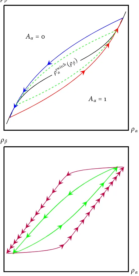
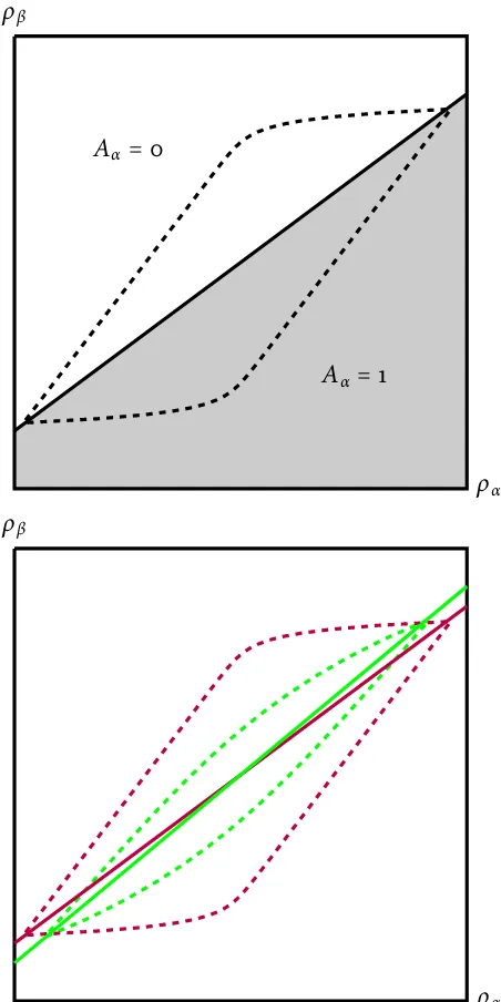
1.3 Outcome paths in stationary equilibria . . . 51
1.4 Stationary equilibria and their corresponding linear strategies . . . 59
1.5 Outcome paths as a function of time . . . 61
2.1 An example of the conditional distributions induced by a rotation order whenγ0>γ1>γ2. . . 89
2.2 When there are no signaling concerns, more informed players than unin-formed players vote.. . . 98
3 Equivalence of the inference problems between a player with uniform beliefs over calendar time, and a player with stationary beliefs over the state. . . 112
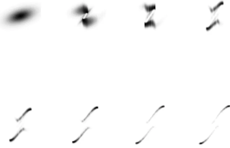
4 Numerical simulation of equilibrium non-stationary distribution. . . 144
5 Numerical simulation of equilibrium non-stationary distribution, part 2. . . 145
6 Numerical simulation of equilibrium non-stationary distribution, part 3. . . 145
Introduction
Fads are a pervasive economic phenomenon, and large industries (advertising, branding,
etc.) exist with the goal of influencing which products are âĂŸin vogueâĂŹ by influencing
who is perceived to be choosing which actions. In chapter one, ‘Fads and imperfect
informa-tion’, I provide a framework to analyze such behavior, grounded in rational agents, and based
on asymmetric information. I model fads as an equilibrium outcome of a dynamic game
with imperfect information. The game has high- and low-type players who differ from each
other in two ways. First, all players want to match the actions of high-types and want not
to match the actions of low-types. Second, the high-type players have access to better
infor-mation about the actions chosen by players in the past—although no player has any special
ability to identify which types chose which actions. The high-type players are interpreted
as a well-connected âĂŸin-groupâĂŹ, and the low-type players as an âĂŸout-groupâĂŹ.
For example, the high-type players may be interpreted as people who live in Manhattan, the
low-types as people who live in a rural area, and the actions as some choice between styles
of clothing to wear. Equilibria of this game display cyclical behavior. Initially, the high-type
is, and start playing it too. Eventually, a tipping point is reached, and the high-type
play-ers switch to coordinate on a different action. They can do so because they are the first to
perceive that an action has become too popular. These dynamics then repeat, with players
periodically switching between actions.
I argue that the model formalizes an intuition about the dynamics of social identity. We
draw credible, positive inferences about well-dressed people—not because they signal their
wealth by buying expensive clothing, but because they signal that they are the sort of people
who understand what one wears in order to appear âĂŸwell-dressedâĂŹ. The key insight of
this chapter is that when the out-group can learn what members of the in-group are wearing,
the meaning of âĂŸwell-dressedâĂŹ must shift over time to remain credible, and the rate
at which it shifts is driven by the speed at which the out-group learns. Equilibria of the
game have surprising properties. Low-type players fail to coordinate on the high-typeâĂŹs
actions because they have access to information which is more âĂŸout-of-dateâĂŹ about
the actions of others. Giving low-type players more up-to-date information causes them to
learn faster, and high-type players to switch more rapidly. The net effect on welfare is zero.
The model, therefore, suggests an explanation for why we cycle through fads more rapidly
today than a century ago: the increasing democratization of information (through radio,
television, social media, etc.) has made it easier for the out-group to learn, speeding up
fads, even if it has not improved their welfare. I show also that low-type players behave as
if they had preferences for conformity. They simply imitate the actions they see were taken
sometimes behave as if anti-conformist. Finally, I consider several extensions to the model.
In one, the in-group has access to older information about the actions of other players; in this
case, they coordinate on actions which appear relatively less popular recently. In another,
players have preferences for appearing to be part of the out-group; in this case, no cyclical
dynamics can be supported, and players simply randomize independently over actions.
Chapter two, ‘Voting as a signal of education’, is motivated by the two facts that voters in
the US are, on average, better educated than the population as a whole, and that self-reported
voter turnout is significantly higher than actual voter turnout. This suggests that there is
a reputational aspect to voting driven by a concern for appearing to be well-informed. I
study voting game in which some players are better informed about the candidates standing
for election. All players have the same cost to voting and preferences for swaying the
elec-tion, and, most importantly, all players have a reputational concern for appearing to be
well-informed through their voting choice. In the game, as the number of players grows large, the
chance of any individual voter swaying the election (the pivot probability) disappears. Voters
endogenously tend to be better-informed than non-voters, and so a large percentage of
play-ers vote—even in large elections—in order to signal their education. The signaling is driven
not be heterogeneity in the cost of voting, but by heterogeneity in voterâĂŹs beliefs about
the value of swaying the election. In contrast to other literature on voting as signaling, the
pivot probability plays an important role in driving voter turnout. The paper thus provides a
resolution to the âĂŸparadox of votingâĂŹ, demonstrating that large levels of voter turnout
quality of all playerâĂŹs information has an ambiguous effect on voter turnout. This result
sheds light on the puzzle that that over the past century, educational attainment in the US
has significantly increased, while voter participation has not, even as voting participation
1
|
Fads and imperfect information
1.1 Introduction
An important feature of consumer choice is that it is observed to shift over time, and in a
way so that choices are correlated among individuals. For example, in the United States in
the 1990s, consumers tended to choose loose-fitted clothing over tight-fitted clothing. In
the 2000s, consumers tended to choose tight-fitted clothing instead. This back and forth in
Western culture can be traced back centuries, to the tight and baggy breeches of
Rennais-sance Europe.
As a positive model of this phenomenom, the standard economic model of consumer
choice is unsatisfactory because it requires us to accept time-varying and correlated
prefer-ences. Such a model is both intractable, and can explain too much behavior. In this paper, I
take a different approach. I analyze a dynamic game between two types of short-lived
play-ers, high and low, each choosing between two equally costly actions, and who differ from
each other in two ways. First, all of the players have preferences for matching the action of
have made the same action choice randomly match with each other, and derive utility from
matching with high type players. Second, the players differ in the quality of information they
possess about the actions of players in the past. I mainly consider the case in which high type
players have better information than low type players about the actions of past players, and
consider other cases in extensions. Players have no special ability to distinguish which types
of players choose which actions, rather, they only observe some information informative
about the relative fractions of players who choose each action in the past. In the body of this
paper, I model this in the following way. I assume that once a player makes an action choice,
their choice (but not their type) is visible for some (stochastic) period of time to other
play-ers. Technically, this corresponds to assuming that players observe a time-weighted average
of past actions. High type players see an average of past actions which places more weight
on more recent actions.
To fix an example, consider the high type players as being those who live in or near
major population centers, and low type players as being those who live in or near rural or
surburban regions, and consider the action choice as being between loose or baggy clothing.
The interpretation, then, is that players prefer to dress like those who live in the city, and that
those in the city have more up-to-date information about the sorts of clothing other players
are wearing. It is not difficult to invent other examples. High type players may be those who
have many friends on Facebook, low type players are those who do not have many friends,
and the choice set is possible news articles to share. Or, high types may be white, low types
applying to a college which wishes to covertly discriminate against Asians.
I focus on stationary equilibria of this game, and I show they may be classified into two
groups. In the first, players mix independently and identically between actions. No
non-trivial dynamics arise from this group of equilibria. Players may all coordinate on one action,
or another, or mix equally between both. In the second, players periodically switch between
action choices. These dynamics are driven by the following intuition. Initially, the high type
players coordinate on an action. Over time, the low type players learn which action the high
type players are coordinating on, and start to choose that action. At some endogenously
determined ‘tipping point’, the high type players switch to coordinate on a different action,
while the low type players continue to coordinate on the ‘old’ action. The high type players
are the first to switch because they are the first to percieve that the trend has ‘played itself
out’. The cycle then repeats, with high type players periodically switching between actions,
and low type players following.
Equilibria of the model have features, broadly consistent with stylized facts, that might
otherwise seem counter-intuitive. Less-informed players mimic the actions they see others
taking, even though they may be mimicking the actions of other less-informed players. In
this sense, less-informed players display instrumental preferences for conforming to the
ma-jority action, even though they do not have direct preferences for conformity. Well-informed
players sometimes mimic the actions they see others taking, and sometimes do not, so that
well-informed players sometimes appear to have preferences for conformity, and sometimes
example: When I go to buy clothing, I tend to buy the sorts of clothing that I see others
around me wearing. An economist observing my choices might reasonably conclude that I
have a preference for conforming to what others are doing, i.e., I prefer to look like those
around me. However, if I go to buy clothing with a fashionable friend, who recommends
I buy a pair of pants that I haven’t seen anyone else wearing, I strictly prefer his
recom-mendation over any choice I would have made. An economist observing my choices in this
case might reasonably conclude the opposite, that I have preferences for anti-conformity,
i.e., I prefer not to look like those around me. In both cases the economist is wrong, my
choices are driven not by any intrinsic preferences for conformity or anti-conformity, but
rather the information available to me about what certain classes of players are wearing. In
this sense, the model considered in this paper is a dynamic extension ofBernheim(1994),
in providing a rationale for the dynamics of conformist and anti-conformist behavior that
is not directly grounded in direct preferences for conformity. In general, we draw negative
inferences about people who are perceived to be conformist; the model suggests a rationale
for why, since only less-informed players consistently act as if conformist.
I show also that the rate at which players switch between actions is driven by the speed
of learning of less-informed players. If less-informed players only learn which action the
well-informed players are coordinating on slowly, then the well-informed players switch
less rapidly. The additional information available to well-informed players, however, has no
effect on the rate at which players switch between actions. It serves purely as a coordination
and end has increased. The shift from Renaissance-era baggy breeches to tight breeches
took centuries, the shift from loose fitting pants in the 2000s to tight fitting pants took a
decade. The model suggests that this phenomenon is driven by two factors. The first is the
increasing visibility of well-informed elites. In the 1600s, this might have been the nobility,
in 1980, it was popular musicians and actors. The second is the increasing democratization
of information. In the 1800s, it may have taken weeks for information to spread among elites.
In 1950, it still took weeks for information to spread among elites. But due to the invention
of widely available sources of information such as broadcast television or the radio, what
took decades to spread among non-elites in the 1800s might have only taken a few years in
1950. Accordingly, the model predicts that the length of fads in the 1800s should have been
on the order of decades, while the length of fads in 1950 should have been on the order of
years.
This democratization of information might have been expected to improve the welfare
of less-informed non-elites. I show that contrary to this intuition, it has no effect on welfare.
On one hand, the less-informed learn faster which action the well-informed are coordinating
on, but on other hand, the well-informed switch more rapidly between actions. Together,
these two effects exactly cancel out.
The model suggests that policies intended to help less-informed players have no effect
on welfare if broadly targeted. For example, some people know that it is customary to wear a
suit to a white-collar job interview. We do not wear suits to job interviews because we want
of person who understands that the sort of thing one does to get a job at a job interview
is wear a suit, and that therefore, we are the sort of person who also understands the other
sorts of things that one does in an office environment to be successful. Telling one person,
who otherwise would have worn a t-shirt, to wear a suit to a job interview might improve
her payoff, telling everyone who might otherwise have worn a t-shirt to a job interview to
wear a suit will have no effect, since the value of wearing a suit to a job interview came only
because it credibly signaled that some people are well-informed.
1.1.1 Previous literature
Previous literature on the switching dynamics considered in this paper (Karni and
Schmei-dler,1990;Matsuyama,1992;Frijters,1998;Caulkins et al.,2007) focus on models in which
cyclical behavior is driven by differences in preferences, or technology (‘conformists vs.
anti-conformists’ or ‘predator / prey’ models).
The paper conceptually closest to this one isCorneo and Jeanne (1999). There, as in
this paper, one sort of player has access to better information than the other, such as the
right restaurant to eat at. Gradually, theβs learn which restaurant is cool, and the authors
analyze the dynamics of this learning process. However, they stop short of considering how
players might switch to other restaurants once everyone has learned where to eat, and how
this might impact the dynamics of the game; in the limit, players end up all pooling on one
action. The major difference to this paper is that inCorneo and Jeanne(1999), players private
players is about the actions of other players, which I show gives rise to equilibrium switching
dynamics.
The question of why we observe fashion and fashion trends is an old one in economics
(Foley,1893). Previous literature on fashion cycles focuses on Veblen goods and
conspicu-ous consumption. InPesendorfer(1995), a monopolist periodically releases new, expensive
clothing lines, giving the wealthy an opportunity to buy expensive clothing to signal their
wealth, then gradually lowers the price of the clothing to sell to more people, before
even-tually releasing a new line of expensive clothing and beginning the process again. Here, the
monopolist is a ‘norm entrepreneur’ (Sunstein,1995), strategically manufacturing social
as-sets for profit. It is true that there are examples of monopolist fashion brands at the high end
of the market—but fashion, and fashion cycles, are a much broader phenomenon, and not
limited to high-end clothing. For example, no norm entrepreneur decided that car tailfins,
which serve no aerodynamic purpose and are no more expensive than conventional styling,
should be popular in the 1950s, and Plutarch (187) describes Cato the Younger wearing a
subdued shade of purple, in reaction to what was then a trend among the Romans of
wear-ing a bright shade of red. Nobody profits from the recent trend towards uswear-ing ‘Emma’ as a
girl’s name, and many fashion trends involve clothing which is deliberately inexpensive.
Other related papers include the literature on social learning (Bikhchandani et al.,1992),
and more specifically the literature on social learning with bounded memory,Kocer(2010).
There, players do not observe (or remember, if players are interpreted as being long-lived)
furthermore, there is no underlying state of the world which players draw inferences about.
The idea behind this paper is the same one behind the literature on supporting correlated
equilibria in static games by modeling them as the result of a dynamic game in which players
condition in some way on the actions of players in the past (Aumann,1987;Milgrom and
Roberts,1991;Foster and Vohra,1997). I apply the same concept, but require player’s learning
process to be Bayesian. For any dynamic (Nash) equilibrium in my model, in any period,
the resulting distribution over action profiles is a correlated equilibria of the static game,
however, the set of correlated static equilibria which can be supported by dynamic equilibria
in this way is much smaller than the set of all correlated equilibria in the static stage game.
Although the empirical study of fads began much earlier, there is a recent interest in
applying modern econometric techniques to identifying fads (Yoganarasimhan, 2012a,b).
The ability to identify the ‘next big thing’ is of obvious interest to firms which sell consumer
products. An industry of ‘coolhunters’ revolves around identifying what will be in fashion
and what will be out of fashion.
In Section1.2, I illustrate the main idea with a simple example model. In Section 1.3, I
describe the stage game, and prove some basic results about equilibria in the static
environ-ment. In Section1.4I describe the full dynamic game. In Section1.4.1, I use analogous results
to those in the static environment to characterize equilibria in the dynamic game. I show
that a feature of all equilibria in the dynamic game is that βplayers show an instrumental
preference for conformity. In Section1.5, I apply the results from Section1.4.1to a
on the period length of the game and the strategies played by α players. In Section 1.6I
consider a generalization of the model in whichαplayers are allowed to have access to older
information about the actions of other players, and players may prefer to mimic βplayers.
In Section2.4I conclude.
1.2 Illustrative example
I begin with a simple discrete time example to illustrate the two major mechanisms driving
equilibrium dynamics in this paper: First, the preferences of players to match high type, but
not low type actions, and second, the better information of high type players. The game
analyzed in this section is simple, but not easily extendable, and so in the main body of the
paper, I consider a richer continuous time model.
Model
Consider a discrete time (t=0, 1, 2, . . .) game. In each period, a continuum of players enters,
each makes a once-and-for-all binary action choicea ∈ {0, 1}, and then each exits.1 With
equal probability, each player is either a high or a low type, denotedθ ∈ {α,β}. Once each
player has chosen an action, a single player is sampled uniformly from the set of players, and
his action choice, denoted at, is made visible to future players. Before a player chooses an
action, he sees a truncated history of past sampled actions. Specifically, a low type player in
periodtsees the past action,at−1. A high type player, on the other hand, sees the pastN>1
actions, (at−1,at−2, . . . ,at−N). (The initial players see no actions, and the second through N −1st players, if the high type, see the entire history.) Hence, the information sets of a
player of typeθin periodt,Ht θ, are
H0
α = {}
H1
α = {(a0)}
H2
α = {(a0,a1)}
Ht
α = {(at−3,at−2,at−1} ∀t≥3
H0
β = {}
Ht
β = {at−1} ∀t≥1.
elements of which are denotedht θ.
Once each player has chosen an action, players randomly and uniformly match with the
other players who chose the same action. Players who choose an action which no other
player has chosen receive a payoff of 0. Players who match with a high type player receive a
payoff of 1. Players who match with a low type player receive a payoff of 0. Players therefore
prefer to choose actions which are more likely to be chosen by high type players, and less
likely to be chosen by low type players.
Player strategies areσθ
t ∶ Hθt → [0, 1], denoting the probability that playert, of type θ,
chooses action a = 1 in period t. A strategy profile induces beliefs, which is a probability
action chosen by that player, denotedµ∈∆(Θ∞× {0, 1}∞). Random variables with respect
to the probability measure representing beliefs are denoted with tildes, so that ˜ht
βrepresents
a low type player’s uncertainty over the previous period action. Formally, a player’s payoff is
1 if and only if he is matched with a high type player, and 0 otherwise. Note that a high type
player who chooses an action expects, at the interim stage, a payoff of
Ut(a,µ,ht
α,hβt) =Pµ(θt=α∣at,at−1,at−2, . . . ,at−N),
that is, a player’s interim expected payoff is the probability that a player randomly selected
from the group of players who choose the same action is a high type player. A low type
player’s interim expected payoff, after choosinga, is then Eµ[Ut(a,µ, ˜hαt, ˜htβ) ∣htβ].
The definition of equilibrium is standard:
Definition ⟨σθ
t,µ⟩is anequilibriumiff
1. Each player is best responding, so thatσt
θ(hθt)has support contained within
arg max
a∈{0,1} Eµ[Ut(a,µ, ˜h
t
α, ˜htβ) ∣htθ],
2. and beliefs, µ, are consistent withσθ
t wherever possible.
Analysis
This simple model captures the two important components of the main game. First, low type
is a coarsening of the high type player’s information. Second, players have preferences for
matching the action which would be taken by high type players, and not matching the action
which would be taken by low type players. Consider the following two candidate strategy
profiles and beliefs, which mirror those analyzed later in the continuous-time game.
Example 1(‘Pooling’ strategy profile). Under this strategy profile, players coordinate on action
1. Formally,
σθ
t(hθt) =1∀θ,t,htθ,
and µ satisfies
Pµ(a0,θ0,a1,θ1, . . . ,at,θt) = ⎧⎪⎪⎪⎪ ⎪⎪⎪ ⎨⎪⎪⎪ ⎪⎪⎪⎪ ⎩
0 ∃i∣ai =0
(1 2)
t
otherwise.
This pooling strategy profile is one in which players coordinate on actiona=1, and
de-viators receive the lowest possible payoff, 0. Unsurprisingly, it is also an equilibrium strategy
profile.
Proposition 1. The pooling strategy profile described in Example 1 is an equilibrium strategy
profile.
Figure 1.1: Two equilibrium path realizations of the pooling (top) and periodic (bottom) equilibria.
On the top, all the players coordinate on one action (represented by black). On the bottom, withN =3, the players coordinate on an action untilN≥3, and a high type player comes along, at which point they switch. (Here, att=3,t=7, andt=10.)
conditional ona=1, is always 1/2, and so for all on-path historiesht α,htβ,
Ut(1,µ,ht
α,htβ) = 21
Ut(0,µ,ht
α,htβ) =0,
and so on-path,a=1 is trivially a best-reply.
Figure 1.1 contains an illustration of the pooling strategy profile. In this case, all the
players pool on one action.
A more interesting strategy profile, which is also an equilibrium strategy profile is the
following:
Example 2(‘Periodic’ strategy profile). Under this strategy profile, low type players mimic the
are the same, in which case, they choose a different action. Formally,
σtβ(htβ) =at−1
σα t(htα) =
⎧⎪⎪⎪⎪ ⎪⎪⎪ ⎨⎪⎪⎪ ⎪⎪⎪⎪ ⎩
1−at−1 at−1= ⋯ =at−N
at−1 otherwise.
It remains to specify the actions of the first N players. The first player uniformly chooses an
action, independently of type. The next N −1players choose actions in the following way:
1. With probability
2(NN−+11) 1
N
−1
the tth player,1≤t<N−1, mimics the previous action, at=at−1.
2. Otherwise, the tth player mixes uniformly between actions.
(The purpose of this somewhat artificial specification of the first N player’s actions is to generate
stationary beliefs. It is not strictly necessary, but assumed for tractability and simplicity.)
Proposition 2. The periodic strategy profile described in Example 2 is an equilibrium strategy
profile when N ≥5.
Proof. First, since playerst=0, 1, . . . ,N−1 choose actions with the same type-independent
is a best reply. Second, I state without proof that the players att=Nbelieve
Pµ(aN−1=aN−2 = ⋯ =ai) = ⎧⎪⎪⎪⎪ ⎪⎪⎪ ⎨⎪⎪⎪ ⎪⎪⎪⎪ ⎩
2
N+1 i=0 1
N+1 otherwise.
(1.2.1)
(In fact, the actions of the firstNplayers were constructed specifically so that (1.2.1) holds!)
Consider first whether the high type players are best responding att =N. In the event
that the pastN players are observed to be choosing the same action, each high type player
knows that each other high type player will be choosing 1−aN−1, and so optimally each high
type player prefers to choose 1−aN−1, receiving an expected payoff of 1 (since only high type
players choose 1−aN−1at this history) instead of 0 (since only low type players chooseaN−1
at this history). In the event that the pastNplayers are not observed to be choosing the same
action, each high type player expects that no other player will be choosing a different action,
and so optimally each high type player prefers to continue to mimic actionaN−1, knowing
that if they choose 1−aN−1, they will receive a payoff of zero, instead of 21 (the probability
that a player choosing actionaN−1is a high type player.) High type players, then, are trivially
best responding at t = N, because choosing the same action as high type players is a best
response.
Now consider whether the low type players are best responding att=N by mimicking
at−1. From (1.2.1), with probability N2+1, the pastN actions are the same, and by mimicking
at−1, a low type player receives a payoff of zero (since all the high type players are choosing
by mimickingat−1, a low type player receives a payoff of 12 (since all players are mimicking
the past action) instead of 0. The low type player’s best reply condition is satisfied, then, if
and only if
2
N+1 ×0+ (1− 2 N+1) ×
1
2 ≥
2
N+1 ×1+ (1− 2
N+1) ×0.
This condition is satisfied if and only ifN ≥5.
Similar reasoning establishes that players are best replying in successive periodst=N+
1,N+2, . . ., if beliefs are stationary. In fact, they are. To see this, fixt, and letPn denote the
probability thatat−n =at−n+1=at−1. Then by construction,
PN =
Probability that lastN−1 were the same
¬
PN−1 +
Probability that lastNwere the same but low type was drawn
¬1
2PN Pn =Pn−1∀1<n<N
P1 =21PN
∑ n Pn=1.
The unique solution for these beliefs is
PN = N2+1
Pn = N1+1∀n<N,
This simple model illustrates the main channel driving periodic dynamics in the main
model of the paper. Low type player mimic past actions, absent a better idea of whether
other players are conforming to the previous action or not. High type players occasionally
conform, and occasionally anti-conform when they percieve that sufficiently many other
players are choosing the same action. In the remainder of the paper, I analyze a richer model,
capable of providing comparative statics results. The main channel, however, is similar.
1.3 Static stage game
A continuum of players, some calledαs and some calledβs, play the following
simultaneous-move stage game. First, nature draws a state,ρ⃗∈ [0, 1]2, from a distributionµ ∈∆([0, 1]2).
Denote the realized state by (ρα,ρβ), and the random variable by (ρ˜α, ˜ρβ). Players then
observe private information: Theαplayers observe(ρα,ρβ), while theβplayers observe only
ρβ. Each player simultaneously chooses an action a ∈ {0, 1}. I focus on symmetric mixed
strategies,2 denoted Aα(ρα,ρβ) ∈ [0, 1]andAβ(ρβ) ∈ [0, 1], mapping private information
into the probability of choosinga=1.
Once players have chosen actions, each player receives a payoff, which is a function of his
2The analysis in the paper goes through if, instead of focusing on symmetric mixed strategies, we were to
focus on pure strategies in which players condition on their index in such a way so that the same fractions of player types choose the same actions. By the law of large numbers, this can always be done. E.g., we could have instead of the symmetric mixed strategyAβ(ρβ), we could have
Aβi(ρβ) =⎧⎪⎪⎨⎪⎪
⎩
1 i≤Aβ(ρβ)
0 i>Aβ(ρβ),
action, and the fraction of players of each type choosing his action. Formally, each player’s
payoff function isU(a,aα,aβ), whereais his action, andaα andaβ are the fractions ofα
and βplayers choosing action 1. Note thatαandβ players have the same payoff function.
Since there are many players, by the law of large numbers we have, in state(ρα,ρβ),
aα(ρα,ρβ) =Aα(ρα,ρβ),
aβ(ρβ) =Aβ(ρβ).
I impose the following assumption on payoffs:
Assumption 1. U(1,aα,aβ) >U(0,aα,aβ)if and only if aα >aβ.
Assumption1 formalizes the intuition that all players strictly prefer an action if more
αthan β players are choosing that action. This may be because players have reputational
concerns for appearing to beαplayers, conditional on the action they take. Or, players may
have intrinsic preferences for choosing the same actions asαs (Akerlof and Kranton,2000),
because they identify withαs but not withβs. Or, after the stage game, players may go on
to play a subgame, the payoffs to which depend on the action chosen in the stage game, as
illustrated in the following example.
Example 3(Matching utility). Interpret the action as a location choice, a =0or a =1, and
introduce a matching subgame in which players are randomly matched to another player at the
drawn player is an α, conditional on the action taken,
U(a,aα,aβ) = ⎧⎪⎪⎪⎪ ⎪⎪⎪ ⎨⎪⎪⎪ ⎪⎪⎪⎪ ⎩
aα
aα+aβ a=1
1−aα
1−aα+1−aβ a=0,
(1.3.1)
On the boundaries, when aα =aβ =0or aα =aβ =1, assume U(a,aα,aβ) =0∀a.3
The payoff specification in Example3will be maintained as an example for the remainder
of the paper.
1.3.1 Equilibria of the stage game
To fix ideas, I derive Bayesian equilibria of the static stage game. There are many such
equi-libria.
The game has trivial equilibria, indexed by p ∈ [0, 1], in which both sorts of players
disregard their private information and mix independently between 0 and 1, each
choos-ing a = 1 with probability p. This follows from Assumption1, which impliesU(1,p,p) =
U(0,p,p) ∀p∈ [0, 1], and so mixing is trivially a best response whenAα(ρα,ρβ) =Aβ(ρβ) =
p.
On the other hand, in no equilibria doαplayers coordinate on action 1 whileβ’s mix, i.e.,
Aα(ρα,ρβ) ≡1,Aβ(ρβ) ∈ (0, 1) ∀ρβ. In this case, it is commonly known thatAα(ρα,ρβ) =1,
and so aα > aβ, hence; by Assumption1,U(1, 1,aβ) > U(0, 1,aβ), and so βplayers strictly
3It is only important thatU(1,a
α,aβ) =U(0,aα,aβ). On the boundaries, these payoffs technically violate
prefer to choose action 1.
Are there equilibria in which theαplayers condition on their additional private
infor-mation in a non-trivial way? More precisely, are there equilibria in which theαplayers, with
positive probability, choose a different action profile than theβplayers? The answer is yes.
To see this, first, we note that in any equilibrium, αplayers are always either all playing 0,
all playing 1, or mixing with the same frequency asβplayers:
Lemma 1. Let⟨Aα,Aβ⟩be an equilibrium strategy profile. Then Aα(ρα,ρβ) ∈ {0,Aβ(ρβ), 1}
for all(ρα,ρβ).
Proof. The result follows directly from Assumption1. IfAα(ρα,ρβ) <Aβ(ρβ), then
U(1,aα,aβ) <U(0,aα,aβ),
and so Aα(ρα,ρβ) = 0 is the unique best reply. Similarly, if Aα(ρα,ρβ) > Aβ(ρβ), then
Aα(ρα,ρβ) =1 is the unique best reply. Finally, ifAα(ρα,ρβ) =Aβ(ρβ)the result holds.
Second, we note that in any equilibrium,βplayers are indifferent between actions:
Lemma 2. Let ⟨Aα,Aβ⟩be an equilibrium strategy profile. Then β players are always
indif-ferent between actions 0 and 1. That is, the following indifference condition is satisfied for all
ρβ ∈ [0, 1]:
P(Aα(ρ˜α, ˜ρβ) =0∣ρβ) × (U(0, 0,Aβ(ρβ)) −U(0, 1,Aβ(ρβ)))
Proof. Fix ˆρβ∈ [0, 1]. EitherAβ(ρˆβ) =0, orAβ(ρˆβ) ∈ (0, 1), orAβ(ρˆβ) =1.
First, ifAβ(ρˆβ) ∈ (0, 1), theβplayers are mixing and so indifferent between actions.
Second, if Aβ(ρˆβ) = 0, then by Lemma 1, Aα(ρα, ˆρβ) ∈ {0, 1}for all {ρα ∣ (ρα, ˆρβ) ∈
Supp(µ)}. Definep0,p1by
pa∶=Pµ[Aβ(ρ˜
α, ˜ρβ) =a∣ρ˜β=ρˆβ], a∈ {0, 1}.
Then a β player’s expected payoff from a = 0 is weakly less than his expected payoff from
a=1, since by Assumption1
p0U(0, 0, 0) +p1U(0, 1, 0) =p0U(1, 0, 0) +p1U(0, 1, 0)
≤p0U(1, 0, 0) +p1U(1, 1, 0),
with strict inequality if and only ifp1 =0. The best response condition then implies thatβ’s
are indifferent betweena=0 and a=1.
The case in which Aβ(ρˆβ) = 1 is analogous. To write the indifference condition, a β
player’s expected payoffs from actionais
E[U(a,Aα(ρ˜α, ˜ρβ),Aβ(ρ˜β)) ∣ρβ]
=p1U(a, 1,Aβ(ρ
β)) +p0U(a, 0,Aβ(ρβ)) + (1−p0−p1)U(a,Aβ(ρβ),Aβ(ρβ)),
impliesU(1,Aβ(ρβ),Aβ(ρβ)) =U(0,Aβ(ρβ),Aβ(ρβ))always) yields (1.3.2).
Combining Lemmas1 and2 together yields the following characterization of
equilib-ria. For ease of exposition, we now assume that µ has full support on[0, 1]2 is absolutely
continuous with respect to Lebesgue measure on the unit square.4
Proposition 3. ⟨Aα,Aβ⟩is an equilibrium of the static game if and only if, for all(ρα,ρβ) ∈
[0, 1]2,
1. Aα(ρα,ρβ) ∈ {0,Aβ(ρβ), 1}and
2. Aβ solves(1.3.2).
Proof. That these conditions are necessary follows directly from Lemmas 1and2and the
fact thatµhas full support on[0, 1]2.
To see that these conditions are also sufficient, note first that if allαplayers are choosing
actiona = 1, then by Assumption1,U(1, 1,aβ) ≥ U(0, 1,aβ) ∀aβ ∈ [0, 1], so that choosing
a=1 is a best reply. Similar reasoning sufficies to show that when allαplayers choosea=0,
it is a best reply for all αplayers to choose a = 0. Finally, when Aα(ρα,ρβ) = Aβ(ρβ), by
Assumption1αplayers are indifferent between actions, and so are best responding. This
es-tablishes thatAα(ρα,ρβ) ∈ {0, 1}is a sufficient condition forαplayers to be best responding.
Forβplayers,1.3.2is the indifference condition, and so every action is a best reply.
For example, consider the special case in which utility is given by the matching subgame,
example3. Letρβ↦g(ρβ)be any mapping into[0, 1]satisfying
Fρβ(g(ρβ)) ∈ (13,23)∀ρβ ∈ [0, 1], (1.3.3)
whereFρβis the cumulative distribution function of the marginal distribution of ˜ραfor some
fixed value ofρβ. Proposition3characterizes equilibria in whichαplayers choose 1 ifρα ≥
g(ρβ), and 0 otherwise.
Proposition 4. Say α’s play according to
Aα(ρα,ρβ) = ⎧⎪⎪⎪⎪ ⎪⎪⎪ ⎨⎪⎪⎪ ⎪⎪⎪⎪ ⎩
1 ρα ≥g(ρβ)
0 ρα <g(ρβ),
(1.3.4)
and β’s play according to
Aβ(ρβ) =2−3Fρβ(g(ρβ)). (1.3.5)
Then under the matching specification of utility,(1.3.1),⟨Aα,Aβ⟩is an equilibrium.
Proof. The proof proceeds by showing that (1.3.5) solves the indifference condition (1.3.2), it
then follows from Proposition3that⟨Aα,Aβ⟩is an equilibrium, since by construction,Aα
g(ρβ)
ρβ ρα
1 1
Aα =1
Aα =0
Aβ(ρβ)
ρβ 1 1
Figure 1.2:Construction of simple static equilibria.
On the left:αplayers coordinate using the (arbitrary) boundary(ρβ,g(ρβ)). On the right: In equilibrium,β
players are more likely to choose action 1 when they believeαplayers are more likely to choose that action.
To that end, note that by construction of theαplayer’s strategy, (1.3.4), we have
Pµ(Aα(ρ˜α, ˜ρβ) =0∣ρβ) =Fρβ(g(ρβ))
Pµ(Aα(ρ˜α, ˜ρβ) =1∣ρβ) =1−Fρβ(g(ρβ)).
The indifference condition then becomes
Fρβ(g(ρβ)) (
1
2−Aβ(ρβ)) = (1−Fρβ(g(ρβ))) (
1
1+Aβ(ρβ)),
solving yields (1.3.5), which is a well-defined strategy only when condition1.3.3is satisfied,
which, by assumption, it is. (WhenFρβ(g(ρβ)) ∉ (13,23),βplayers strictly prefer one or the
This equilibrium is one in which theαs have exclusive access to some hidden ‘sunspot’,
which allows them to coordinate on an action, represented by the value ofρα. (Sinceρβonly
ever takes one value, theβ-type players have access to no private information.) For example,
imagine that ρβ represents broadcast television, while ρα represents cable television, and
people who can afford to watch cable television would like to choose the same action as
other people who can afford to watch cable television. The model suggests they can do so by
coordinating on the information they see through cable television. In equilibrium,βplayers
are aware that this coordination is taking place, and must draw inferences about which action
αplayers are coordinating on.
The function g(ρβ)determines how likely it is that αplayers will choose actiona =1.
The lower is g(ρβ), the greater the probability that, conditional on ρβ, the α players are
coordinating on actiona=1. Theβplayers equilibrium strategy, (1.3.5), is also decreasing in
g(ρβ). In this sense,βplayers are mimickingαplayers, but the degree to which this occurs is
driven byβplayers beliefs about the extent to which otherβplayers are choosing an action.
What are the expected payoffs to players under the strategy profile described in
Propo-sition4? LetVα andVβdenote theex-anteexpected payoffs to each type of player, i.e.,
Vα ∶=Eµ[Aα(ρ˜α, ˜ρβ)U(1,Aα(ρ˜α, ˜ρβ),Aβ(ρ˜β))
+ (1−Aα(ρ˜α, ˜ρβ))U(0,Aα(ρ˜α, ˜ρβ),Aβ(ρ˜β))]
Vβ∶=Eµ[Aβ(ρ˜β)U(1,Aα(ρ˜α, ˜ρβ),Aβ(ρ˜β))
Thenαplayers can do well, as summarized in the following result:
Proposition 5. Let⟨Aα,Aβ⟩be any equilibrium in which Aαis determined by(1.3.4)for some
boundary g. Then
Vα =2Vβ,
and under the matching specification of utility,(1.3.1), Vα = 23 and Vβ = 13.
Proof. The full proof is in AppendixA.1; here I present an intuitive proof. By construction,β
players are indifferent between strategies, by construction, hence, aβplayer who randomizes
50/50 between actions receives the same payoffex-anteas in equilibrium. Half the time, such
a player chooses the same action as anαplayer and receivesVα, half the time he does not
and receives a payoff of zero, therefore,
Vβ= 12Vα.
When payoffs are induced by the matching subgame, (1.3.1), the payoff to a player is the
ex-pected probability that the player is anα, conditional on his action, so, theex-anteprobability
that a player is an αshould equal the expected payoff of players, and since the probability
that a player is anαplayer is 1 2,
1
2 =
1 2Vα+
1
2Vβ=Vβ+ 1 2Vβ=
soVβ= 13 andVα =23.
Surprisingly, the payoff to anαplayer in equilibrium is independent of the strategyAα,
as long asAα(ρα,ρβ) ∈ {0, 1}. In the next section, I augment the model so that state variable
evolves and is allowed to depend on past actions, in such a way so that over timeβplayers
can eventually learn which actionαplayers are coordinating on. Do the features of the static
game carry over into the dynamic environment? In sections1.4.1and1.5I show that they do:
αplayers can still condition on their private information, and can extract the same payoffs in
the dynamic game that they do in the static game. I show that this occurs when behavior is
cyclical — in order to extract the same payoffs,αplayers need to periodically switch between
actions. Furthermore, I show how the dynamic structure of the game induces particular
forms for g(ρβ),µ, and the β’s strategy; I give intepretations of these forms and analyze
comparative statics.
1.4 Dynamic game
Now, time is continuous, t ∈ [0,∞). In each instant t, a continuum of short-lived players
play the static game. The state space is still the unit square,[0, 1]2, but elements of the state
space are now denoted ρt = (ρt
α,ρtβ), to represent the dependence on time. I maintain the
assumption that bothαs andβs observe the value ofρt
β, but that onlyαs observeρtα. Again,
imagine that ρt
β represents a source of information available to everyone in the game, such
broadcast television, while ρt
of the population, such as cable television.
The game proceeds as follows. First, an initial condition is drawn from µ0 ∈ ∆[0, 1]2.
I denote the random variable by ˜ρ, andρ0 is the realized initial condition. Given an
ini-tial condition ρ0, the game outcome path is action paths at
α(ρ0),atβ(ρ0) and state paths ρt
α(ρ0),ρtβ(ρ0) for t ∈ [0,∞), where, analogously to the static game, atα and aβt are the
fractions of α and β players choosing action a = 1 at time t. For convenience, the
de-pendence on the (stochastic) initial conditions will be omitted where it is clear, so that
the (stochastic) value of the outcome path at time tis denoted(a˜t
α, ˜atβ, ˜ραt, ˜ρtβ)to represent
(at
α(ρ˜0α, ˜ρ0β),atβ(ρ˜0α, ˜ρ0β),ρtα(ρ˜0α, ˜ρ0β),ρβt(ρ˜0α, ˜ρ0β)).
It will be of interest to consider two special sorts of outcome paths. A pointρ∗is afixed
pointunderρtif
ρt(ρ∗) =ρ∗∀t∈ [0,∞).
A pointρ∗is aperiodic pointif there existsP>0 such that
ρP(ρ∗) =ρ∗,
and the minimum suchPis called theperiod. The set of states traced out by the state path is
called theorbit. An orbit is calledfixedif it consists of a single fixed point, andperiodicif it
Information structure
We would now like to impose a dynamic structure on the game to capture the idea thatρtis
somehow representative of actions taken in the past. To do so, I now impose the following
interpretation on the meaning of ρt. When players make an action choice, I assume that
the choice (but not the player’s type, or the time at which they chose the action) is visible
for some time afterward. Although a player’s type is not known, I assume one type’s action
choices may be more visible than others. Imagine, for example, that once a player chooses
which style of clothing to wear, they wear it for some stochastic, exogenous amount of time
before replacing it, at which point their choice is no longer visible.5The value ofρt
αrepresents
the fraction of players observed to be ‘wearing’a=1 at some location where the replacement
rate of old clothing is higher than at some other location, represented byρt
β. I assume that old
action choices disappear at some exogenous Poisson raterα andrβ, respectively. Formally,
the change in the fraction of players observed to have been choosinga =1, for small time
increments, evolves approximately according to
ρt+ε
α ≈ (1−εrα)ρtα+εrα(λαatα+λβrtβ)
ρt+ε
β ≈ (1−εrβ)ρβt +εrβ(λαatα+λβrtβ).
5When the player replaces his clothing, we could imagine that he returns to the game and makes a new
Here, λαatα +λβatβ is some average of the actions being taken by each player type. λα and
λβ are intratemporal weights, parameterizing how visible a particular player type’s action
choices are. Accordingly, we takeλα +λβ = 1 andλα,λβ >0. Whenλα is large,ραt andρtβ
mostly reflect the actions of high types, conversely, whenλβis large,ραt andρtβmostly reflect
the actions of low types.
While λα and λβ are interpreted as intratemporal weights, rα andrβ areintertemporal
weights, adjusting how rapidly it is that old actions disappear. Consistent with the
interpre-tation above, I assume thatrα >rβ >0, so that ρtα represents a more ‘up-to-date’ average of
the actions being taken.
In the limit asε→0, we derive
˙ ρt
α =rα(λαaαt +λβatβ−ρtα) (1.4.1)
˙ ρt
the laws of motion ofρ⃗t.6A solution to (1.4.1) and (1.4.1) is
ρt
α =e−rαtρ0α+rα∫ t
0 e
−rα(τ−t)(λ
αaτα+λβaτβ)dτ (1.4.3)
ρt
β =e−rβtρ0β+rβ∫ t
0 e
−rβ(τ−t)(λ
αaτα+λβaτβ)dτ, (1.4.4)
which makes explicit the fact that we assume that ρ⃗tis an exponentially-weighted moving
average of past actions, with weightsrα andrβ, up toρ0, the initial condition.78
This specification ofρ⃗t captures the idea that players have some information about the
actions of other players, but that this information is delayed, and does not immediately
re-flect changes in action choices. The assumption thatrα > rβ captures the idea that the αs
have access to more up-to-date information thanβs, since a higher value forrαplaces more
weight on more recent actions.9
6More generally, we might specify that(ρt
α,ρtβ)evolve according to some law of motion which depends
on the action profile,
˙ st
α= fα(ραt,atα,atβ)
˙ st
β= fβ(ρtβ,atα,atβ),
in which case fα(ρα,aα,aβ) =rα(ρα−λαaα−λβaβ), fβ(ρβ,aα,aβ) =rβ(ρβ−λαaα−λβaβ)corresponds
to an exponentially weighted moving average; the assumption thatρα,ρβare exponentially weighted moving
averages is tractable and has a simple interpretation compared to the general case.
7There is some ambiguity as to the meaning of a solution to a discontinuous differential equation,
which (1.4.1), (1.4.2) may be. Here, I mean a Carathéodory solution, that is, the solution should satisfy
st = ∫ t
0 s˙
τdτ+s0.
8An alternate way to have set up the model would been to have had time begin at−∞, which motivates
an interpretation ofρ0
α,ρ0βas representing, in some reduced-form way, the state of the system at time 0.
9An exponentially weighted moving average is, of course, simply one out of many which we could have
Strategies
A strategy profile is now functions mapping calendar time and the observed state variable
into the probability of choosing action a = 1, denoted Atα(ρ
α,ρβ),Atβ(ρβ). A strategy is
stationarymeans it is independent of calendar time,At
α =Aα,Atβ =Aβ∀t∈ [0,∞).
A strategy profile⟨At
α,Atβ⟩, induces an action path through—analogously to the static
setting—the conditions
at
α =Atα(ραt,ρtβ) (1.4.5)
at
β=Atβ(ρtβ)∀t∈ [0,∞) (1.4.6)
from the law of large numbers; it induces a state path through the laws of motion (1.4.3), (1.4.4).10
Payoffs
For a fixed outcome path, the payoffs to a player in periodtare the same as in the static game,
that is, if a player chooses actionaat timet, his payoff isU(a,at
α,aβt), satisfying
Assump-tion1. A player who sees private informationsupdates his beliefs over initial conditions, as
10Outcome paths satisfying (1.4.5), (1.4.6), (1.4.3), and (1.4.4) are neither guaranteed to exist, nor to be
unique. In the case where an outcome path does not exist, as may occur, for example, if Aα orAβ are not
previously noted, for every initial condition there is a unique outcome path, hence, beliefs
over initial conditions induce beliefs over the value of the outcome path at every time t. I
denote random variables with tildes and realizations without tildes.
Equilibrium
An equilibrium consists of a strategy profile and beliefs over the state variable at each time
t, denoted⟨At
α,Atβ,µt⟩, such that players are best responding to their beliefs, and beliefs are
consistent with the outcome path induced by⟨At α,Atβ⟩.
Formally, players are best responding given beliefs when (note that the expectation
op-erator is omitted forαplayers, since their belief updating process is trivial)
Supp(At
α(ραt,ρtβ)) ⊆arg max
a∈{0,1} U(a,a
t
α,atβ) (1.4.7)
Supp(At
β(ρtβ)) ⊆arg max a∈{0,1} Eµ
t[U(a, ˜aαt, ˜atβ) ∣ρ˜tβ=ρβ] ∀t∈ [0,∞) (1.4.8)
and beliefs are consistent with equilibrium behavior when, for all measurable subsets S ⊂
[0, 1]2,
µ0(S) =µt(ρtα(S),ρt
β(S)) ∀t∈ [0,∞). (1.4.9)
An equilibrium is stationarymeans the strategy profile and beliefs are stationary, so that
At
α = Aα,Atβ =Aβ, and µt = µ∀t ∈ [0,∞). Stationarity does not imply stationarity of the
1.4.1 Equilibria of the dynamic game
I formally state a characterization of stationary equilibria in this game and discuss its
impli-cations. The full proof is in the appendix.
Proposition 6. Let⟨At
α,Atβ,µt⟩, be an equilibrium. Then, for all t,
1. At
α satisfies
At
α(ρ˜α, ˜ρβ) ∈ {0,Atβ(ρ˜β), 1}and (1.4.10)
2. At
β(ρβ)solves
Pµt(Aα(ρ˜αt, ˜ρtβ) =0∣ρ˜βt =ρβ) × (U(0, 0,Atβ(ρβ)) −U(1, 0,Atβ(ρβ)))
=Pµt(Aα(ρ˜αt, ˜ρtβ) =1∣ρ˜tβ =ρβ) × (U(1, 1,Atβ(ρβ)) −U(0, 1,Atβ(ρβ))) (1.4.11)
Furthermore, these conditions are sufficient for equilibria, in the following sense: Let⟨At α,Atβ⟩
be a strategy profile, and say µt are probability distributions over[0, 1]2 consistent with the
outcome path induced by⟨At
α,Atβ⟩. If for all t ∈ [0,∞), ρα,ρβ ∈Supp(µt), it is the case that
Aα(ρα,ρβ)satisfies(1.4.10)and Aβ(ρβ)satisfies(1.4.11), then⟨Atα,Atβ,µt⟩, is an equilibrium.
Proposition6is simply a re-statement of Lemmas1and2, from the static environment in
the dynamic environment. If we require equilibria to be stationary, we can derive stronger
Proposition 7. Let ⟨Aα,Aβ⟩, µ be a stationary equilibrium. Then, for allρ⃗∈ Supp(µ), Aα
satisfies(1.4.10), Aβ solves
∣λα+λβAβ(ρβ) −ρβ∣ × (U(0, 0,Aβ(ρβ)) −U(1, 0,Aβ(ρβ)))
= ∣λβAβ(ρβ) −ρβ∣ × (U(1, 1,Aβ(ρβ)) −U(0, 1,Aβ(ρβ))) (1.4.12)
almost surely, and λα+λβAβ(ρβ) −ρβ ≥0and λβAβ(ρβ) −ρβ ≤0.
Furthermore, these conditions are sufficient for equilibria, in the following sense: Let⟨Aα,Aβ⟩
be a stationary strategy profile. If for allρ⃗∈ [0, 1]2, it is the case that A
α(ρα,ρβ)satisfies(1.4.10)
and Aβ(ρβ)satisfies (1.4.12), then there exists a probability measure µ on [0, 1]2 such that
⟨Aα,Aβ,µ⟩, is a stationary equilibrium.
Propositions6and7look similar, and so it is worthwhile to consider their differences.
Proposition 6is the dynamic version of Proposition3, and the proof is similar. In
Propo-sition 3, µ was taken to be exogenous. Proposition6 has nothing further to say about µt
beyond the equilibrium requirement that it be consistent with player’s behavior. For
sta-tionary equilibria, however, it is possible to say more about µ. Specifically, the marginal
distributions Pµt(Aα(ρ˜tα, ˜ρtβ) = 0 ∣ ρ˜tβ = ρβ) and Pµt(Aα(ρ˜tα, ˜ρβt) = 1 ∣ ρ˜tβ = ρβ)may be
characterized, which yields (1.4.12), and furthermore, given strategy profiles⟨Aα,Aβ⟩
satis-fying (1.4.10) and (1.4.12), Proposition7states that consistent equilibrium beliefs exist, while
Proposition6has nothing to say about the existence of consistent beliefs for a given strategy
A focus on stationary equilibria is often justified through an argument that they
repre-sent, in some way, the long-run of a non-stationary equilibrium of the game. Since I mainly
focus on stationary equilibria for the rest of the paper, in AppendixA.2I show via
numer-ical simulation that it is not unusual for non-stationary equilibrium behavior to result in
convergence to a stationary equilibrium.
1.4.2 Instrumental preferences for conformity
Under the matching specification of utility, it is possible to explicitly characterize
equilib-rium strategy profiles in stationary equilibria forβplayers by applying (1.4.12) from
Propo-sition7:
Example 4(Matching utility I cont.). Here,
U(a,aα,aβ) = ⎧⎪⎪⎪⎪ ⎪⎪⎪ ⎨⎪⎪⎪ ⎪⎪⎪⎪ ⎩
aα
aα+aβ a=1
1−aα
1−aα+1−aβ a=0,
when aα ≠0or aβ≠0, and0if aα =aβ =0. Then equation(1.4.12)becomes
rβ(ρβ−λβAβ(ρβ)) ×1+ (1−1Aβ(ρ
β)) =rβ(ρβ−λα−λβAβ(ρβ)) × 1
1+Aβ(ρβ), (1.4.13)
Solving yields
That is, under the matching specification of utility, β players mimic the actions they see have
been taken in the past. It is not clearex-antethat β players should display this behavior, after
all, they do not have direct preferences for conformity, in the sense that their payoffs are not
necessarily increasing in the number of other players choosing the same action. Is this a general
feature of the model, or is it specific to the matching specification of utility? In this section, I
argue that it is a general feature of the model, in the sense that β players are more likely to
take an action the more they see that other players have chosen that action in the past, in every
stationary equilibrium.
An interpretation of equation (1.4.14) is that theβplayers are ‘endogenously’ conformist.
Their strategy could be interpreted as the players sampling an action from the social network
represented by ρβ, and mimicking it. In fact, this induced preference for conformity is a
feature of the general model:
Proposition 8 (Instrumental preferences for conformity). Say ⟨Aα,Aβ,µ⟩ is a stationary
equilibrium. If ρβ,ρ′β are two draws fromρ˜β and ρ′β > ρβ, then with probability 1, Aβ(ρ′β) ≥ Aβ(ρβ).
Aβ(ρ′
β) <Aβ(ρβ). Then, by Assumption1, we have
U(1, 1,Aβ(ρβ)) <U(1, 1,Aβ(ρ′β))
U(0, 1,Aβ(ρβ)) >U(0, 1,Aβ(ρ′
β))
U(0, 0,Aβ(ρβ)) >U(0, 0,Aβ(ρ′
β))
U(1, 0,Aβ(ρβ)) <U(1, 0,Aβ(ρ′
β)),
and so
U(0, 0,Aβ(ρβ)) −U(1, 0,Aβ(ρβ)) >U(0, 0,Aβ(ρ′
β)) −U(1, 0,Aβ(ρ′β)) (1.4.15) U(1, 1,Aβ(ρβ)) −U(0, 1,Aβ(ρβ)) <U(1, 1,Aβ(ρ′
β)) −U(0, 1,Aβ(ρ′β)). (1.4.16)
On the other hand, (recall by Proposition7thatλβAβ(ρβ) −ρβ≤0,λβAβ(ρ′β) −ρβ ≤0):
∣λα +λβAβ(ρβ) −ρβ∣ ≤ ∣λα+λβAβ(ρ′β) −ρβ∣ (1.4.17)
∣λβAβ(ρβ) −ρβ∣ ≥ ∣λβAβ(ρ′β) −ρβ)∣. (1.4.18)
Together, (1.4.15), (1.4.16), (1.4.17), and (1.4.18) contradict (1.4.12), which holds with
proba-bility 1, and so it must be with probaproba-bility 1 thatAβ(ρ′
β) ≥Aβ(ρβ), the desired result.
That is, with two independent draws from ˜ρβ, it is almost certain that theβplayers will
for conformity, rather, it arises from strategic incentives on the part of players to appear to
have better information about the actions of other players. It provides a rational for why
we might observe aesthetic preferences for conformity, and furthermore, why preferences
for conformity might be viewed negatively by others, or associated with lower-class tastes
(Bourdieu,1984).
1.5 Matching game application
In this section, I apply Proposition7to explicitly compute equilibria in the case where payoffs
are determined by the matching subgame, as in example 3. Imagine that player’s action
choices are interpreted as a choice between locations (for example,a=0 represents a bar on
the east side of town, anda=1 represents a bar on the west side of town). Once players have
made the action choice, they travel to the location, and look for someone to match with.
Matching with anαresults in a payoff of 1, and matching with a βresults in a payoff of 0.
Say in addition that instead of unit masses of both sorts of players, there is a mass Mα ofα
players andMβofβplayers. The payoff of a player who chooses actionais therefore derived
using Bayes’ rule as
U(a,aα,aβ) =P(Meeting anα∣Choosinga)
=⎧⎪⎪⎪⎪⎪⎪⎪⎨⎪⎪⎪ ⎪⎪⎪⎪ ⎩
Mαaα
Mαaα+Mβaβ a=1
Mα(1−aα)
Mα(1−aα)+Mβ(1−aβ) a=0.