The Epoch of Reionization: Foregrounds and Calibration With Paper

(1)

University of Pennsylvania

ScholarlyCommons

Publicly Accessible Penn Dissertations

Summer 8-12-2011

The Epoch of Reionization: Foregrounds and

Calibration With Paper

Daniel C. Jacobs

University of Pennsylvania, [email protected]

Follow this and additional works at:http://repository.upenn.edu/edissertations

Part of theCosmology, Relativity, and Gravity Commons, and theInstrumentation Commons

This paper is posted at ScholarlyCommons.http://repository.upenn.edu/edissertations/362

Recommended Citation

Jacobs, Daniel C., "The Epoch of Reionization: Foregrounds and Calibration With Paper" (2011).Publicly Accessible Penn Dissertations. 362.

(2)

The Epoch of Reionization: Foregrounds and Calibration With Paper

Abstract

Nearly half a billion years passed between the release of the now routinely observed Comic Microwave Backrgound and the formation of the first galaxies and black holes which reionized the ubiquitous hydrogen. This Epoch of Reionization (EoR) is the next major unexplored cosmological milestone. At the current time the space between galaxies is almost completely ionized, therefor we know that the universe must have undergone a global phase transition. The nature of the ionizing sources, whether young galaxies or accreting massive black holes is unknown. Neither do we know when this reionization occured or how long it took. Models suggest that we can detect fluctuations in the 21cm hydrogen emission line as ionization proceeds and high contrast ionized holes are carved in the neutral hydrogen. Detecting these fluctuations is one of the few direct probes of the reionization process but is a difficult task requiring a new generation of low frequency radio telescopes. Motivated by the breadth of unknowns, the Precision Array for Probing the Epoch of Reionization (PAPER) has been slowly building in complexity while folding the results of observations back into improving the design and operation of the telescope. As part of this process, this thesis analyzes early observations to explore three major areas of concern in detecting EoR: contamination by foreground sources, calibration stability and limiting sensitivity. Catalogs produced from this early data show good agreement with previous measurements. We conclude that the calibration is stable and sensitivity floors are close to the expected theoretical levels.

Degree Type

Dissertation

Degree Name

Doctor of Philosophy (PhD)

Graduate Group

Physics & Astronomy

First Advisor

James Aguirre

Keywords

Epoch of Reionization, Cosmology, radio interferometry, 21cm

Subject Categories

(3)

THE EPOCH OF REIONIZATION:

FOREGROUNDS AND CALIBRATION WITH PAPER

Daniel C. Jacobs

A DISSERTATION

in

Physics and Astronomy

Presented to the Faculties of the University of Pennsylvania in Partial Fulfillment of the Requirements for the Degree of Doctor of Philosophy

2011

James Aguirre,

Supervisor of Dissertation

Charlie Johnson, Graduate Group Chair

Dissertation Committee:

(4)

COPYRIGHT

2011

Daniel C. Jacobs

This work is copyright under the

Creative Commons Attribution-NonCommercial-ShareAlike 3.0 License

To view a copy of this license, visit

(5)

This thesis has benefited beyond measure from the help, advice and pointed criticism of many people who are actually not too numerous to thank. Naturally none of this would have been possible without team PAPER: Aaron Parsons, Jonnie Pober, David Moore, Rich Bradley, Nicole Gugliucci, Pat Klima, and Erin Benoit. My South African friends Carel van der Merwe and Jason Manley were exquisite hosts in all capacities as were invaluable interns Tandeka, Charity, Freedom & Gerard. Ngiyabonga kakhulu! PAPER was the brain-child of Don Backer, an amazing person who took a chance with me. He was an honest and gentle role model who is sorely missed.

During the course of this work I benefited immensely from specific contributions by others that are worth calling out. David Moore overcame his natural enmity with computers to write a very nice CASA data converter, Jonnie Pober suggested the faceting that resulted in a fabulous all-sky map and Aaron Parsons invented, then carefully explained delay transforms and spearheaded the (ongoing) sensitivity calculations. In places of subtle genius their hand is clear; any mistakes are my own.

Thank you to my committee for taking on yet another student and setting aside part of your brain for radio astronomy. Though for James Aguirre I must reserve the largest measure of my gratitude. Thank you for taking me on and then trusting me to follow my family back across the country to finish this work in New Mexico.

Though the west would present its challenges. This thesis would have been unfinished without the brave people who fought the Las Conchas forest fire threatening Los Alamos while I finished the last chapter. Thanks for saving my town.

During the past few years my family really shone. Sister Becky, you cheered without flagging. Mom, thanks for the commiserations. There were many times when you said exactly the right thing. You won the PhD race! Thanks for helping me to the finish line. Dad, you are kind, gentle and wise. Thanks for the phone calls, they were some of the finest procrastination a son could ask for.

(6)

ABSTRACT

Daniel C. Jacobs

Supervisor: James Aguirre

Over the last 20 years we have learned that the contents of the universe are spit into 76% Dark Energy and 24% Matter, 17% of which is ordinary matter. Of the ordinary matter the bulk is hydrogen which forms the raw material for building stars. The universe began 14 Billion years ago with an expanding space-time and quickly began After about 300,000 years this all cooled enough for the plasma to recombine into neutral hydrogen gas and release photons which we eventually observe redshifted into the radio; the Cosmic Mi-crowave Background (CMB). Nearly half a billion years passed before the slow process of gravitational collapse would lead to the formation of the first galaxies and the (re) ion-ization of the ubiquitous hydrogen. This Epoch of Reionion-ization (EoR) is the next major unexplored cosmological milestone. At the current time the space between galaxies is al-most completely ionized, therefor we know that the universe must have undergone a global phase transition. The nature of the ionizing sources, whether young galaxies or accreting massive black holes is unknown. Neither do we know when this reionization occured or how long it took.

(7)

List of Tables

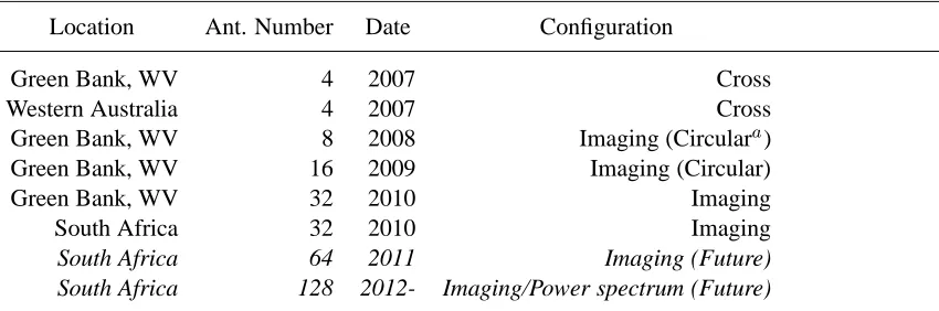
2.1 PAPER deployments . . . 29

2.2 PSA32 Observations . . . 34

2.3 A comparison between AIPY and CASA . . . 36

3.1 Low frequency surveys . . . 38

(10)

List of Figures

1.1 Global evolution of the CMB, gas and Kinetic temperatures (via Pritchard

& Loeb (2008)) . . . 7

1.2 A slice through a model of 21cm brightness temperature showing evolu-tion with redshift. . . 8

1.3 A summary of the EoR power spectrum: models, sensitivity, and data . . 9

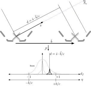
1.4 Basic interferometer operation: The delay in arrival time between wave-fronts corresponds with a peak in the spectral Fourier transform ”delay space”. . . 11

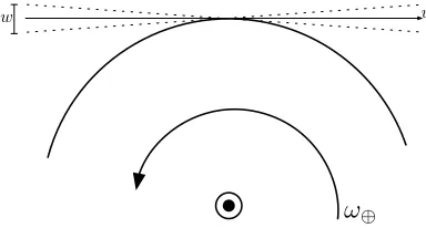
1.5 Snapshot approximation: Over a ten minute snapshot the w term of the baseline vector is much smaller thanuandv terms. . . 13

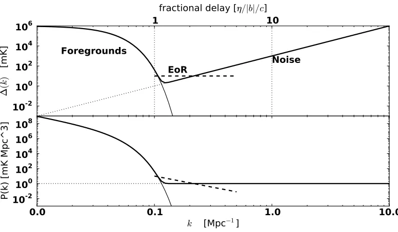
1.6 A power spectrum schematic: foregrounds, noise, EoR . . . 16

1.7 The relationship between foregrounds and EoR power. . . 18

1.8 The dimensions of the power spectrum measured by PAPER (adapted from Morales & Wyithe (2010)). . . 20

2.1 Labeled photo of a PAPER station . . . 26

2.2 Schematic diagram of PAPER . . . 27

2.3 A perpendicular cut through the PAPER primary beam at 150MHz . . . . 30

2.4 Aerial photo and configuration map of PAPER South Africa 32 element imaging array . . . 31

2.5 uvdistribution of PSA32 imaging configuration . . . 31

2.6 Point-spread function (PSF) of the PSA32 ”dirty beam”. . . 32

2.7 RFI survey of PAPER South Africa Site . . . 33

2.8 RFI flagging in South Africa . . . 34

3.1 Comparison between NVSS catalog values and NVSS points as given in Helmboldt. . . 42

3.2 Distribution of delay solution used for PSA32 catalog . . . 43

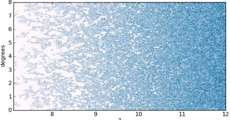
3.3 PSA32 sky coverage. . . 45

3.4 Declination and LST survey coverage . . . 46

3.5 A PSA32 wide bandwidth image centered at 22h-30d. . . 48

3.6 PAPER additions to two interesting spectra. . . 49

(11)

3.8 Section of PSA32 sky survey image near 5h 0d, showing corruption from

Crab low in the beam . . . 51

3.9 Catalog fluxscale map. . . 52

3.10 PAPER’s flux scale distribution . . . 53

4.1 Effect of delay calibration on imaging. . . 58

4.2 Key regions of the sky and the de Oliviera-Costa/Haslam smooth sky model. 59 4.3 Pictor A field. . . 60

4.4 EoR fields with CASA calibration and imaging. . . 61

4.5 Fornax A. Resolved as a double lobed radio galaxy. . . 63

4.6 Bandpass phase solution modeled as a single delay and a phase offset. . . 64

4.7 Delay solutions over 11 days are remarkably stable. . . 65

4.8 Relative amplitude solutions over 11 days are also very stable. . . 66

4.9 Centaurus A as imaged by PAPER 160MHz compared with new ATCA+Parkes mosaic . . . 67

4.10 The system temperate spectrum and time dependence: model and data. Deviation of the correlation temperature from the system temperature. . . 70

5.1 The delay spectrum of a typical but steep spectrum source with some RFI flagging is well isolated by the polyphase filter bank/CLEAN combination. 74 5.2 A model of foregrounds in a wide-band delay transform. . . 75

5.3 Integrating noise on a simulated correlation. . . 78

5.4 The single baseline, unit variance power spectrum and its integration prop-erties in minimally processed data. . . 79

5.5 Cross-talk is stable. . . 81

5.6 Removing a long time average is effective. . . 83

(12)

Preface

Sometime about 14 Billion years ago the universe began with a hot big bang. We now know that the universe was endowed with a certain amount of energy which is divided be-tween dark energy, dark matter, photons and baryons most of which was hydrogen plasma. After 300,000 years or so this plasma cooled enough for the electrons to recombine with the protons and release the photons of the Cosmic Microwave Background. After the first billion years the first stars, galaxies and black holes had formed into the objects we recognize today.

Observations of the CMB have verified this cosmological picture while deep integra-tions with optical and infrared telescopes have pushed closer to the birth of stars and galaxies. Despite these efforts, much remains unknown about the first billion years of evolution. In particular, we know very little about the first stars and galaxies. Were they massive and bright? Where they numerous but dim? Where the first galaxies anything at all like we see in more recent times? We see tantalizing hints of early galactic evolution at later times but, occasionally these facts are at odds. The period between the CMB era and the earliest observed galaxies is completely uncharted territory.

One of the last truly global events is the (re)ionization of hydrogen. It is certain to have happened, we observe that the bulk of the hydrogen is ionized to very high redshift yet must have been neutral for the CMB to propagate. Hydrogen emits a narrow spectral line at 21cm which we observe redshifted to several meters, near the commercial FM radio radio band. This transition is theoretically detectable with a sensitive telescope operating between 100 to 200 MHz. Ideally this telescope would image the gas at narrow redshift slices and so get a complete 3D image cube. This is out of reach of current technology, but even a relatively modest telescope may measure the power spectrum which is made bright and distinctive by the high contrast ionized holes in the neutral gas. Detection of hydrogen as it undergoes this process would be the highest redshift yet seen, a significant discovery. It is an ideal probe of early star and galaxy formation processes and an ideal compliment to traditional stellar astronomy.

(13)

of the sky, making it an ideal instrument for a power spectrum measurement, but existing telescopes do not have enough elements to achieve the desired sensitivity. The Precision Array for Probing the Epoch of Reionization (PAPER) is one of several radio interferom-eters now under construction with the goal of detecting the power spectrum of hydrogen undergoing reionization. It is the only interferometer built solely for this purpose.

The design of the instrument is dictated by the need to cover a wide range of redshifts and therefor a wide bandwidth, but also achieve a high sensitivity and therefore a large number of antennae. This results in a challenging amount of data and a very wide band-width. To simplify calibration and minimize instrumental effects, the antenna must have a smooth spectral and spatial response. When combined with cost constraints these require-ments result in a small element with a very wide field of view that breaks a number of common simplifying assumptions used in radio inteferometry.

All of these problems are scaled by the ever increasing size of the array with the cor-relation of N antenna scaling everything by N2_{. This work explores the data from 32} antennae. Only a year later we are now collecting 64 antenna data which is larger by a factor of four. Assuming no improvement in analysis tools the fraction of data we are able to explore will decrease by the same amount.

Radio astronomy has a long tradition of imaging. Despite our almost exclusive interest in the power spectrum, there are still several good reasons to image as well. If the data are faulty, error-prone or mis-calibrated this is very difficult to tell by direct examination, partly because of the sheer volume of correlation measurements and partly because of the unintuitive nature of interferometric measurements. Successful imaging is a powerful argument for instrumental stability.

However, in an array that is starved for sensitivity, imaging is in direct competition with measuring the power spectrum. In an interferometer the positions of the elements de-termine the Fourier modes measured. A power spectrum measurement must first measure each Fourier mode to good sensitivity which necessitates an arrangement that minimizes the number of independent modes sampled while an imaging array is optimal when it max-imizes the number of modes sampled. These two requirements are in tension. We believe that we must observe in both imaging and power spectrum configurations to characterize the instrument and foregrounds and to achieve a power spectrum detection.

The large number of elements, the large bandwidth and necessity of balancing imaging with measuring the power spectrum are some of the difficulties with which we must con-tend. We can not nor need not fully investigate each problem with the same level of detail. The PAPER experiment approach is to investigate and solve problems as they come up and save money by only solving problems that need to be solved. These lessons will eventu-ally inform the building of much larger telescopes where such an approach would not be possible. In this thesis I embrace this approach by investigating recent PAPER observa-tions performing the first level of checks for problems that would prevent us from reaching design sensitivity. In this thesis I try to answer this question using early observations from the PAPER instrument taken during its extended construction period.

(14)

students and engineers. This small group operates mainly out of the US with around two deployments to South Africa per year. Beginning in 2007 PAPER has yearly increased the size of the array by a factor of 2 with a goal of 128 elements in 2012.

PAPER’s copper pipe dipole antennae, amplifiers, plastic pipe reflector frames and correlator are fabricated in the US and shipped to South Africa where we assemble them into an interferometer. Throughout the past three years I have had many opportunities to work with the instrument in the field. In addition to several outings to the test array in Green Bank, WV I was a key member of two of the past four deployments to South Africa. In October 2009 I was first on site to break ground and work the assembly and deployment effort for the first 16 dipoles. I led the effort to calibrate the positions of the elements using precision GPS surveying equipment and held primary responsibility for array position configuration. As a member of a three person team I worked a second deployment in May 2010 to commission the now 32 element array and make the first observations.

During this time it was common for more data to be produced than could be analyzed in detail. This thesis goes some small way to rectifying this situation by providing both an image and power spectrum analysis of the two problems most likely to affect an EoR detection: foregrounds and sensitivity.

The foregrounds are addressed by imaging the sky and extracting a catalog. To show that this is the output of a stable instrument, I compare the catalog fluxes and positions to those previously recorded and find a reasonable match. Not only did this prove the instrument was more stable than was previously thought, it also provided the first new measurements of many of these sources in almost 50 years. In the power spectrum domain I show via simulations and real data that if foregrounds are smooth as expected then they can be isolated from the region of power spectrum we would like to measure. As part of this I explain in more detail that the power spectrum measured by PAPER is almost entirely in the spectral domain i.e. the Fourier transform of the frequency spectrum. Careful transformation along this axis is key to foreground isolation, but unstable calibration or poor sampling along the spectral axis can swamp the measurement.

To get a better look at the calibration I brought the data into another analysis pipeline where time dependent solutions, among other things, were possible. To do this I worked closely with the Nation Radio Astronomy Observatory scientists and software engineers and organized the effort within PAPER including setting up several project workshops at the VLA operations and science center in Socorro, New Mexico. The result of this analysis was the first proof that the calibration heretofore assumed to be stable, actually was. As an additional validation of this pipeline I also generated several images of interest to observers.

(15)

and thus has a spectral slope and is time variable. In addition, the variance in the cross-correlations is not necessarily proportional to the system temperature. Indeed this turned out to be the case for the upper half of the band. I do not theorize about this discovery; more investigation is warranted. It is sufficient to say that it might be indicative of a kind of noise that does not integrate down as thermal noise.

For this reason I explore the ability of just a single baseline to integrate down as it should. With only rudimentary data processing the noise integrates down with some re-maining residual. Though, If we hope to integrate for 100 times longer more work is left to be done in identifying the limiting factors.. There are enough hints and approximations made that this can probably be achieved in the current data but with new and better data coming soon from the latest 64 antenna deployment our focus will most likely shift in that direction.

This catalog and the work published in this thesis is the first and possibly last look at 32 antenna PAPER data. It is a snapshot in time of the project and a rare glimpse into a project moving quickly towards its goal. Hopefully it will go some small way to providing the interested observer a better idea of where we are, the promise of the data and maybe some hints about where we are going.

(16)

Chapter 1 The Epoch of Reionization

1.1 In the beginning...

The story of the Epoch of Reionization begins, as all stories must, with the Big Bang. Here was the beginning of time as we know it; a universe filled with copious amounts of ionized Hydrogen (and Helium) plasma, black body photons and hugely inflated quantum density fluctuations. All of which were extremely hot and embedded in an expanding space-time. At these temperatures and densities the Hydrogen plasma was in thermal equilibrium with the photons; the free electrons scattered the photons making space opaque. Time passed and the Universe cooled. After about 300,000 years the number of photons above 13.6eV drops below the number of baryons and Hydrogen began to capture electrons. The plasma was neutralized and photons were free to proceed a few of which were eventually observed by us as the Cosmic Microwave Background (CMB; Loeb & Barkana (2001).

Freed of its connection to photons, the Hydrogen (HI) pursued its own gravitational interests. Density fluctuations began to slowly accrete gas into what would eventually be clusters of galaxies. At the same time the hydrogen began to radiate, including a very long lived transition emitting photons 21cm long, which unfortunately appear to us, redshifted1 as they are by intervening spacetime expansion, to have the unreasonable wavelength of 230 meters. At these wavelengths the ionosphere is completely opaque, the IGM is in free-free absorption and above redshift of 150 the HI emission is invisible against the CMB. Save these few radio waves and other similar atomic lines, no radiation is thought to have been generated for the next 500 million years until the birth of the first stars.

Thus began the time period known colloquially as the Dark Ages which was ended by an enlightenment of stars and AGN beginning around a redshift of 20, lasted around 700 million years and eventually resulted in the complete RE-ionization of Hydrogen.

But of course the Dark Ages were not dark. By redshift 20, the observed HI wavelength is only 4 meters, a challenging but not impossible observation. Here we will explore the

1_{Redshift (}_z_{) is the inverse of the expanding Universe’s scale factor (}_z _{= 1}_/a_{) where a goes from zero}

(17)

global evolution during the beginning of the end for HI. We will find that the stars drive the HI to have a distinct global spectrum ending in an Epoch of Reionization (EoR). We know HI is currently ionized but models give a range of redshifts at which reionization could have reached 50%. Establishing the redshift at which the universe is 50% ionized (zreion) is a goal of current EoR experiments (Furlanetto et al., 2006; Morales & Wyithe,

2010).

Constraining zreion could answer many questions about the origin of stars, galaxies

and massive black holes. Is a hierarchical model of galaxy formation correct? How does feedback affect star formation? What kind of fossils might remain today? Many of these questions can be constrained by single observable: When did the IGM re-ionize?

1.2 Observing the EoR

Evidence from absorption of quasars and the CMB indicates that the EoR most likely oc-curred between redshifts 6 and 14 (Furlanetto et al., 2006; Fan et al., 2006), but even this broad limit assumes a fairly simple ”instantaneous” model of the transition. The Gunn-Peterson troughs caused by Lyαabsorption of quasar spectra provide a sound lower limit ofz _≈6. However the Lyαline quickly saturates at relatively small neutral fractions (Fan et al., 2006). This effective limit in redshift space is compounded by the lack of decent statistics; we are limited in the number of pierce points by the number of known quasars at high redshift. Most recently observations of quasar ULASJ112001.48+064124.3 at z=7.085 (ν21 = 175MHz) have been found to be consistent with a neutral fraction of 0.1 or greater (Mortlock et al., 2011).

In concert with other cosmological measurements, polarized Thompson scattering of the CMB provide an optical depth of free electrons, a measure of the age of our ionized IGM. The measure is consistent with a instantaneous re-ionization process sometime be-tween9< z < 14or a gradual, multi-stage process with a first stage at12< z < 17and a second near z _≈ 7. Like the quasar and other absorption estimates the best constraint provided by the CMB is on the end of re-ionization. Instantaneous ionization atz = 6has been ruled out to 99.9% confidence level (Dunkley et al., 2009).

Galaxy surveys, particularly with the Hubble Space Telescope, have begun to produce estimates of star formation rate and photon escape fraction at higher redshifts. These few measurements of total radiation and star formation history at high redshift are also domi-nated by strong selection limitations and other errors. Together their estimates of ionizing radiation suggest that there was probably enough Lyman-continuum radiation from stars to ionize the the IGM (Robertson et al., 2010). Deeper observations might reduce the un-certainty in this measurement. A good sample would require a much deeper survey in the near-IR by James Webb Space Telescope or a 30m class ground-based telescope. However these observations cannot by themselves establish the stars as the cause of reionization, nor will they be able to easily probe higher redshifts. Galaxy surveys in a universe where gaseous Hydrogen is the dominant baryonic matter are only part of the story.

(18)

spin-flip transition radiates a very narrow-band spectral line that allows precise determination of relative velocity, which for these distances is dominated by the Hubble flow, giving us a precise distance measure. Because of its low optical depth, this 3D probe traces both mass and temperature via its intensity but also provides a high-contrast probe of the ionization process and has been recognized as a very potent observable for everything from cosmology to galaxy formation and IGM astrophysics.

Direct detection of HI during reionization remains elusive. To-date only relatively un-likely scenarios have been ruled out. The single antenna EDGES experiment (Bowman & Rogers, 2010) has been able to eliminate ”fast” reionizationdz <0.05at good confidence while Paciga et al. (2011) have made GMRT observations (see Fig 1.3) that rule out a fairly unlikely cold reionization (described below).

In the absence of any detection of high redshift hydrogen we are limited to best guesses from partly analytic and partly numerical simulations that track density, temperature and ionization fronts. Broadly, these models agree that as more objects radiate UV photons, ionization regions will increase in size eventually percolating through all space leaving only small islands of neutral hydrogen in deep, galactic-scale, gravity wells. These models provide a target sensitivity for detection efforts as illustrated in Fig 1.3. Most models agree to within a factor of 2 onzreionand predict a somewhat wider spread of amplitudes.

Several EoR experiments are currently operating, including the Murchison Widefield Array (MWA; Lonsdale et al. 2009), the Low Frequency Array (LOFAR; R¨ottgering et al. 2006), the Giant Metre-wave Radio Telescope (GMRT; Paciga et al. 2011), and the Pre-cision Array for Probing the Epoch of Reionization (PAPER; Parsons et al. 2010). Here we will focus on PAPER, an experimental meter wave interferometer under construction in South Africa.

The first detection of 21cm radiation in 6 _≤ z _≤ 13 will put a date on ionization of various size scales by constraining the power spectrum amplitude and redshift Bittner & Loeb (2011). Later experiments will measure the shape of the power spectrum from which we can learn about the matter and velocity distribution, as well as details about the ionization process and cosmological initial conditions (Lidz et al., 2007). In particular the deviations from spherical symmetry can constrain the initial power spectrum to put limits on inflation (Bowman et al., 2007). Imaging the spectral line signal is more challenging yet and is forecasted to start to be possible with arrays 10x the size of those currently under construction while full 3D imaging needs 100x, a enormous scale usually referred to as a Square Kilometer Array (SKA).

1.3 Theory

Like the CMB, much can be gleaned from the global spectrum of HI as it evolves. The brightness temperature of the 21cm (Tb) line depends on couplings between the population

(19)

n2 n1

= 3 expT⋆ Ts

and available energy sources. The HI emission is viewed in contrast to the CMB photon field

Tb ⋍29mK

1 +z

10

Ts−TCM B

Ts

(1 +δm)χH

and is modulated by the gas densityδmand the ionization fractionχH.

In the absence of energy sources like stars the temperature of the HI line is limited to coupling with either the cosmological matter (Tk) or photons (TCM B). The temperatures

of these reservoirs drop as the universe expands until the birth of the first UV and Xray sources begins to significantly heat the gas. Eventually it succumbs to ionization.

The evolution of HI temperature has been analytically calculated by Pritchard & Loeb (2008) as shown in Figure 1.1. After recombination (z _∼ 1100) there were enough free electrons left over to couple the gas to the CMB photons (Ts = TCM B) but byz ∼ 300

these were absorbed by the increasingly cool gas. At this early time the matter density is still high enough to collisionally couple the spin state to the gas kinetic temperature (which is colder than the CMB by a factor of(1 +z)−1_{) paradoxically putting the line into} absorption with the CMB (Ts ∼ TM < TCM B). Eventually, probably aroundz ∼ 70, the

gas became too rarified to collisionally couple and the HI was once again dominated by the black body CMB photons (Tb =TCM B).

This state of things continued until the very first stars began to radiate (z _∼20₋30). First the X-Rays and then UV photons from these early objects pump the 21cm transition via the Wouthuysen Field Effect (WFE) into states that are more sensitive to the gas tem-perature which for a time means returning to the cooler gas temtem-perature (Ts = TM). As

time progresses the growing number of radiation sources raises the gas temperature into the emission regime Ts ≫ TCM B before finally beginning the ionization process where

the ionization fraction quickly grows to unity and the differential brightness temperature quickly drops to zero. Note that If the heating is so fast that the gas transitions nearly instantaneously from cold to ionized (so-called ”cold reionization”) the amplitude of the differential brightness will be much larger (100mK of absorption instead of 30mK of emis-sion). This is the scenario probably ruled out by Paciga et al. (2011).

Figure 1.1 depicts this global history for various models of star formation. Driven primarily by relatively simple cosmological scale physics, the early portions are fairly well constrained by current cosmology. The various models tend to agree. However there is a wide range of reionization end-points (sreion). As we can see from the variety of

end-points, measurement of the end of reionization would provide the strongest constraint on these models.

(20)

traces out its own history in a poorly understood relationship with the underlying dark and baryonic matter. Star formation depends on the abundance of metals in the early IGM as well as the thermal-kinetic flows of matter into and around dense regions. Quasar formation depends on the formation and evolution of massive black holes. These multiple interacting timelines act together to drive the temperature and ionization state of each point in the IGM through through the phase transition atzreion.

While the higher redshift global spectrum is simpler to predict, the later period of re-ionization is richer in information for the same reason that it is difficult to model. The EoR band is also the highest redshift that can be observed from the ground where the ionosphere is still transparent and Radio Frequency Interference (RFI) can be avoided be observing from a remote location. Despite these relative advantages many difficulties must still be overcome, beginning with an initial detection of high redshift HI.

Early EoR experiments do not have the sensitivity to detect or image localized HI emission but must combine observations of multiple regions into a single measurement of the emission power spectrum. The first generation of these experiments is further limited to providing constraints on portions of this power spectrum, for example by looking for a peak in HI variance predicted to occur as re-ionization reaches the halfway point (Bittner & Loeb, 2011).

Generically speaking the power spectrum of a re-ionization model tells a simple story. A simulation by Matt McQuinn (Figure 1.2; McQuinn personal communication, 2010) that includes evolution, tells the story. Before ionization begins the power spectrum is simply the average temperature times the density. A power law distribution, increasing toward smaller scales. Ionization begins with small bubbles forming around, rare massive objects, adding power at largekwhich will percolate to larger scales as the bubbles expand. By the time ionization fraction reaches 50% most ionization regions will overlap and the variance will peak. After the halfway point the IGM will become a series of shrinking HI islands in a sea of HII. As they shrink power will move back to smaller scales but with an increasingly diminishing average level.

To put limits on the set of possible re-ionization histories with these early observations we must have in hand models suitable for comparison to measurement that sample a wide range of possible scenarios. Sampling both in angular and frequency space, early experi-ments will measure scales of 0.1 to 100 Mpc and measure how the power spectrum evolves over the half-billion years of first star formation (20 > z > 6). Theoretical efforts have focused on gross estimates with analytical methods (Loeb & Barkana, 2001; Pritchard & Loeb, 11), detailed fully numerical and semi-numerical combinations thereof.2 Each flavor samples a continuum between precision and statistical significance. Relevant to our cur-rent observations are their predictions of the evolution of the 21cm brightness temperature power spectrum. Analytical models of the power spectrum easily predict over all relevant scales but are limited in their ability to constrain non-linear affects such as the shape of HII regions or velocity perturbations. To be statistically significant numerical models must span a region much larger than the largest HII zone but have resolution small enough to

(21)

identify sources of radiation. Simulations that most accurately solve the full hydrodynam-ics of the IGM and propagation of the ionizing radiation are not quite currently technically feasible on these scales (Zahn et al., 2010). Current work has focused on semi-numerical methods that compromise between the twin desires of generating many simulations and increasing their accuracy (Zahn et al., 2010; Santos et al., 2010; Mesinger et al., 2011) such as the simulation by McQuinn shown in Figure 1.2. Spanning a size of 1300Mpc and including evolution over a redshift range from 12 to 7 this simulation represents the state of the art and approaches the size scales measured by PAPER. However there is only one. Most simulation work has focused on comparing results from different methods; and in consequence have made efforts to use the same initial conditions and physical processes.

Of course these difficulties are moderated by the need to predict on the scale of the lim-ited sensitivity of early experiments. Even with the limlim-ited variability within simulations, there is enough spread in possible amplitudes to make a rough estimate of the possible constraints an experiment could offer. As can be seen from Figure 1.3, PAPER will have the ability to constrain a fraction of current models.

Though exploration of different re-ionization scenarios has been limited, several classes of scenarios have emerged as coarse testable areas. These are divided into ”early” and ”late” which are hypothesized to coincide with hard spectrum Quasars and softer small cool stars, respectively. Furthermore, a Quasar dominated spectrum would manifest as an ”outward in” percolation from rare regions in contrast to a star dominated epoch of reion-ization ”inside out” transition with more regions acting as nucleation sites for HII bubble growth(Zaldarriaga et al., 2004).

Constraints on these histories will require detection and constraint of the power spec-trum at multiple scales and redshifts. A reasonable expectation for PAPER, given existing models, is that it will eliminate late (low-redshift) models that predict the most power on small scales as ionization reaches the halfway point.

1.4 High z HI observing

1.4.1 Comparison to CMB

(22)

(23)

(24)

10-2 ₁₀-1 ₁₀0 ₁₀1 ₁₀2

|k| [Mpc1]

10-2

10-1

100

101

102

103

104

105

k3

P

(T

k

)

/

2

[

mK

]

Foregrounds

santos 2010 zahn 2010 mesinger 2010 furlanetto 2006 PAPER128 MWA512 SKA paciga 2010

7 8 9_z 10 11 12

|k|0.1Mpc

1

(25)

elapsed between the discovery by Penzias & Wilson (1965) and precision measurement of the black body spectrum by COBE. Operating in space, COBE’s FIRAS instrument compared the sky temperature to a precision calibration source in a relatively noise-free band to measure the spectrum to one part in 105_{. In the case of the EoR neither the} signal level nor the transition band-width are well constrained. EoR experiments with no knowledge of the amplitude can not with certainty estimate signal to noise ratio making the design sensitivity a matter of guesswork. Foregrounds are at least five orders of magnitude above the signal and RFI is epidemic3. Finally EoR (a 3D signal which varies with time) is fully twice as many dimensions as the 2D CMB. It fills all more of the spectrum with its signal leaving fewer data points with which to make an uncontaminated measure of the foregrounds. Surely the goal is worthy but the road is long, longer maybe than we might expect if we are comparing to the CMB.

Given that we cannot confidently set the parameters of the experiment with safe pre-cision we must prosecute our search more carefully. In addition to our ignorance of the target amplitude we must overcome serious observational challenges about which we are also ignorant. Astronomy in this frequency range is complicated by large physical size (1 to 3 meters), the wide field of view that comes from using small cheap elements and the large number of elements necessary to achieve the requisite sensitivity. These telescopes must correlate thousands of channels over hundreds of elements; a difficult technical chal-lenge. The large Field of View (FoV) and >100% fractional bandwidth strain or break many of the interferometrists simplifying assumptions. Yet the instrument must be ex-ceptionally precise to distinguish between EoR and 100,000 times brighter foregrounds. Confirmation of EoR fluctuations will require exquisite understanding of both instrumental and foreground effects. This suggests that a careful program of sky model and instrument improvement are essential elements of a path to detection.

1.4.2 The Fourier Domain

Interferometric measurement

An interferometer measures the correlation between the electric fields measured by a pair of antennae separated by distance (or baseline) vector~b. On a quiet night, these electric fields are dominated by astronomical radiation I(ˆs from directionsˆ, the wavefronts pro-ceeding regularly across the array. In the limit of parallel wavefronts from a single distant source the correlation is given by the field power multiplied by the complex phase rotation the wave undergoes as it propagates the additional geometric distance (sˆ_·~b)between the two antennaeiandj(See Fig 1.4.

Vij =I(ˆs, ν)e−2πisˆ·~bν/c (1.1)

3_{The observation that EoR is might be a more difficult observation than the CMB was originally made}

(26)

−1 +1

df

η

+_b/c −b/c

d= ˆ_s_·!_b/c

Beam

F

!b

ˆ

s

d=

ˆ

s·!b/c

S_s

(27)

Of course the sky is full of sources, both continuous and discrete so we must integrate over the entire sky to find the total correlated power.

Vij =

Z

I(ˆs, ν) exp [₋2iπˆs_·~bν/c]dΩ (1.2)

The baseline is often written in wavelengths~u =~b/λ = (u, v, w), and the sky vector in cosinessˆ= (l, m,√1₋l2₋_m2₎_where_l _{= cos(}_φ_{) cos(}_θ₎_and_m_{= sin(}_φ_{) cos(}_θ₎_if_θ_and φare elevation and azimuth, respectively. Another way of reckoning the correlation phase is that it is the geometric delay, the extra travel time, experienced by the light between the two antennae,d= ˆs_·~b/c

Vij =

Z

I(l, m, ν) exp [₋2iπ(ul+vm+w√1₋l2₋_m2_)]_dldm/√₁₋_l2₋_m2 _(1.3)

WhereIis the intensity at sky position cosinesl, mandu, v, ware the relative coordinates of the two antennae iand j, measured in wavelengths. These are the coordinates in the frame of the sky, and thus rotate with the earth once every sidereal day. The integral is the sum of the correlated electric fields from all points on the sky where the field due to each point on the sky has a different geometric delayd= (ˆs_·~u).

At the moment of correlation the electric field has been amplified by each antenna differently. Each antenna has an overall amplitude calibrationa(ν)which changes counts to volts, and also has a relative phaseφ(ν). This phase is dominated by an electrical delay d; a phase changing linearly with frequency (φ =dν).

gi(ν) =a(ν)eiφ(ν)≈a(ν)eidν (1.4)

Finally, the antenna has its beam pattern, a direction dependent gain A(ˆs, ν)to go inside the integral, which we will assume to be similar for each antenna. Combining all of these we get a complete relation between the sky and the output of the interferometer.

V_ijo =gigj

Z

A2(l, m, ν)I(l, m, ν)e

[−2iπ(ul+vm+w√1−l2 −m2

)] √

1₋l2 ₋_m2 dldm (1.5) commonly referred to as the ”visibility”.

Given a model or measurements of the sky, beam, and baseline vectors we can integrate the right hand side, to get a model visibilityVm

ij which is related via complex gains to the

observed visibility and can be written as a matrix equation,

Vo₌GVmG _(1.6)

Where the rows and columns of V_ij _{are the antenna correlations, while the diagonal}

ele-ments ofG_{are the gains. From here there are a variety of methods available for producing}

(28)

increas-u w

ω_⊕

Figure 1.5: For a flat array, the wcomponent is instantaneously zero and over a longer period of time is approximately zero. This period of time we refer to as the ”snap-shot” which for PAPER is about 10 minutes. For illustrative reasons we have exaggerated the angles by a factor of 10.

ingly accurate knowledge of the sky is traded for a better gain solution.

As we will see, with certain simplifying assumptions measuring the correlation of the sky gives us access to both the flux distribution and the power spectrum with only a Fourier transform along the appropriate axes. Next we will quickly explore these approximations, use the results to relate the theoretical power spectrum to our measurement and finally estimate the necessary sensitivity level and the stability required to meet it.

To the power spectrum

Even without the complication of instrumental calibration, the peculiar quantity measured by the interferometer itself is, at first glance, of limited use. The complicated interaction of the round sky, the flat array, and the change in effective baseline length with time and frequency makes deconvolution ofI troublesome. However, a careful examination of the magnitude of the terms in the baseline vector, sky direction dot productsˆ_·~uallows us to make several simplifying approximations.

First, consider the output of our transit interferometer. Each sample measures a slightly different pointing ˆs(t)but we would like to image or compute power spectra with many samples toward a common pointingˆs0. To do this we can rotate to a coordinate system of the sky, where the the pointing stays the same but the array rotates.

ˆ

s(t)_·~u= (ˆs0+δsˆ)·~u(t) (1.7)

Our array is laid out on a uniform graded surface and is approximately flat. Whenˆs(t) = ˆs0 the w or vertical component of the baseline vector is zero. Afterdtseconds the w term has increased by cos(δ) sin(dtω_⊕). At the north pole (δ = 90◦₎ _w_{is always zero. As an} extreme example consider a 300 meter East-West baseline (the maximum length possible with PAPER) on the equator (see Fig. 1.5. Neglecting thew-term as the pointing rotates through _∼ 3% of the PAPER field of view, over 10 minutes, we incur a 4% error in our estimate of the phase.

(29)

approxi-mation

Vij =

Z

A2(l, m)/√1₋l2₋_m2_I₍_{l, m}_{) exp [}₋₂_iπ₍_ul₊_vm_)]_dldm _(1.8)

Looking ahead at our antenna beam pattern (Fig. 2.3), we see that the beam width of 40◦is much less than the size of the sky, the√1₋l2 ₋_m2 _{component. In other words we} may approximate that

A2(l, m)_≈ A

2₍_{l, m}₎ √

1₋l2₋_m2 (1.9)

which at 20◦amounts to an error of 4% and is known as the ”flat sky” approximation. Together these two approximations have linearized our measurement equation

Vij =

Z

A(l, m)I(l, m) exp [₋2iπ(ul+vm)]dldm (1.10)

which is now directly measuring the 2D Fourier transform of the sky. The image of the apparent skyA_∗Iis just a Fourier transform away! Of course we aren’t interested in the image. We want the full three dimensional Fourier transform, where the spectral domain gives us distance via the Hubble relation. Returning to our notation from Equation 1.2

Vij =

Z

A2(l, m)I(l, m, ν) exp [₋2iπ(bxl+bym)ν/c]dldm (1.11)

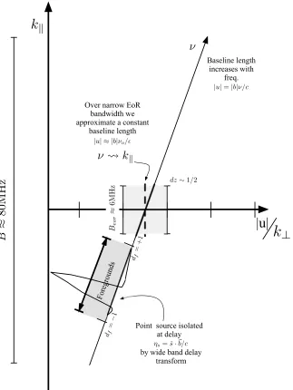
The uvν are coordinates the space defined by the Fourier sky plane extended in the red-shift direction. The uv coordinates are frequency dependent; a single cross-correlation spectrum (baseline) samples uvν space at a radial slant. Strictly this would mean that a baseline does not exactly lie ”along” the line of sightkmode (k_k), however it is close. The largest range over which evolution could be considered static at these redshifts is usually assumed (Furlanetto et al., 2006; Morales & Wyithe, 2010) to be aboutdz 1/2or 6 to 8 MHz. Assuming the worst case of 8MHz of bandwidth at 110 MHz observed on our 300 meter baseline ignoring the wavelength dependence of a baseline length incurs a 7% error in the phase, somewhat larger than but reasonably commensurate with the flat-sky approx-imation. Ignoring the frequency dependence of a baseline is not significantly different than making the usual flat-sky approximating. Thus, as we illustrate in Fig. 1.7, we may extend our approximation to thezdimension.

Using this ”Flat Space” approximation we set the frequency dependent baseline~bν to have its mean value ~u = ~bν0. We are now able to take the Fourier transform in the frequency direction

˜

V(u, v, η)ij =

Z Z

I(l, m, ν) exp [₋2iπνη]dνexp [₋2πilu+mv]dldm (1.12)

(30)

spectrum.4_{. Substituting the measured units}₍_{u, v, η}₎_{for the physical wavenumber vector} ~k = (~k_⊥, k_k), converting to temperature units and squaring we find the relation between power spectrum and

ˆ

V_ij2(η)_≈

2kB λ2

2 _V

X2_Y Pb(~kij). (1.13)

Where 2kB λ2

2

converts from Kelvins to Janskys, X and Y convert angle and frequency to distance, and V specifies the volume (Mpc3) integrated to get Pb(~k). In the case of our observation this is proportional to the volume of space probed by the product of field of view Ω and bandwidth B. Here we convert to cosmological coordinates using the approximate relation used by Furlanetto et al. (2006) which is consistent with the WMAP5 cosmological parameters (Dunkley et al., 2009)

X _≈1.9

1 +z 10

0.2

h−1 Mpc

arcmin (1.14)

Y _≈17

1 +z 10

1

2 Ω

mh2

0.15

−1

2 Mpc

MHz, (1.15)

where forΩm = 0.26the volume conversion becomes

X2Y _≈540

1 +z 10

0.9

h−3 _Mpc3

sr_·Hz (1.16)

. The power spectrum quantity most commonly computed by theorists is the total power in a radially logarithmic bin of a symmetric power densityPb(~k)

b

∆2(k)_≡ k

3

2π2Pb(~k) (1.17)

Switching to this representation, our power spectrum becomes

ˆ

V_ij2(η)_≈

2kB λ2

2 _V

X2_Y

2π2 k3

ij

b

∆2(kij). (1.18)

∆2₍_k₎ _{could be any of the many recent predictions, including those above. As noted} above, there is still some disagreement among models of the 21cm power spectrum owing to uncertainties about the timing of reionization and the strength of star formation. Given this uncertainty we won’t belabor the selection of a prediction beyond the fact that all are in rough agreement with (at most) 10mK of power at k > 0.1Mpc−1 occurring at some redshift between 7 and 11. Most importantly it provides a way to relate the noise in a visibilityVN to the power spectrum noise level∆2N.

(31)

10-2

100

102

104

106

(k

)

[

mK

]

_Foregrounds

Noise EoR

1

fractional delay [

10

/|b|/c

]

0.0 0.1 1.0 10.0

k

[Mpc

1

]

10-2

100

102

104

106

108

P(k) [mK Mpc^3]

(32)

1.4.3 Noise Power Spectrum

An interferometer with field of viewΩwill have a noise componentVN with amplitude

|V(ν)ij,N|=

2kB

λ2

TN,rmsΩ (1.19)

integrating over bandwidth to get the delay spectrum just adds a bandwidth term

˜

V(η)ij,N =

2kB

λ2

TN,rmsΩB (1.20)

TN,rmsis the temperature after integrating over bandwidthB, timet, and two polarizations TN,rms = Tsys/2Bt. Combining Eqs 1.20 and 1.18 we arrive at an estimate of the noise

contribution to the power spectrum for a single baseline

∆2_N(k)_≈X2Y k 3

2π2

Ω 2tT

2

sys, (1.21)

1.4.4 SNR

The sensitivity of the entire array depends on the sensitivity of a single baseline, the num-ber of independent samples of each k mode (oruvpixel) and the number of modes sam-pled. Here we derive the sensitivity of single baseline and relate the net sensitivity given the PAPER configuration found in a recent study to have the highest SNR on a single~k mode (Parsons et al., 2011).

To calculate the sensitivity given in Eq. 1.21 we need only estimate the total integration time for a single baseline measuring a singlekmode. Sampling an angular size1/_|u_|our baseline will observe a fraction1/_|u_|/√Ωof the sky in one earth rotationt_⊕ for a coher-ence time oft_⊕/_|u_|√Ω. For a fiducial baseline of 20 wavelengths (133ns) this corresponds to about 10 minutes, during which time we may average visibilities before squaring them which after 120 nights will reach:

∆2

N(k)≈2.8×104

k 0.1hMpc−1

3

Ω 0.76 sr

3 2 × Tsys 500 K 2 120 days tdays

|~u_| 20

mK2, (1.22)

A sensitivity giving us an SNR of (at best) _≈ 10−2_{. Naively this means we would need}

(33)

|u|

k

_⊥ dz_∼₁/₂

ν

!

k

!

Point source isolated at delay

Baseline length increases with

freq.

|u_|=_|b_|_ν/c

ν

ηs= ˆs·"b/c by wide band delay

transform

k

_!

Over narrow EoR bandwidth we approximate a constant

baseline length

|u_{| ≈ |}b_|_νo/c

B

≈

80M

Hz

B

eo

r

≈

6M

Hz

df =−

1 df

= +1

Foregrounds

Figure 1.7: A single baseline at frequency ν samples a basline of length_|u_|corresponding to the

(34)

angle. As was pointed out by Halverson (2002), in the limit where we do not achieve an SNR_≥ 1on each mode, our noise will only decrease as1/N12 as we average independent ~ks whereas the noise in power spectra withSNR _≥ 1samples will average as 1/N. Thus it is in our best interest to get as close as possible to that 100 measurements per~k-mode number before combining power on different~ks.

To do this with a limited number of antennae we must select an array that maximizes the number of similar baselines. After comparing the redundancy of several configura-tions, Parsons et al. (2011) selected a grid of 11 columns separated by 20 wavelengths (10m @150MHz) having 12 densely packed rows. This configuration, given the above single baseline sensitivity, will achieve a theoretical sensitivity of ∆2

N(k) ≈ 33mK2 at k = 0.1hMpc−1 or an SNR of_≈ 3. In summary: For each baseline we must be able to average the same 10 minutes of sky for 120 days decreasing as 1/t the entire way to ≈ 1/N = 5 _× 10−5_{, or} _≈ ₄₅_{dB. In Chapter 5 we will test PAPER’s ability to} inte-grate as 1/N and examine the importance of various instrumental effects and our ability to ameliorate these problems in post-processing. An integration this deep is challenging, particularly with a relatively simple instrument, however, as we’ve seen in our derivation of the power spectrum sensitivity, the geometrically flat nature of the EoR power spec-trum means that the most sensitive part of the power specspec-trum is also the closest to the foregrounds which also merit careful study.

1.4.5 Foreground Power Spectrum

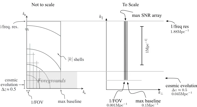
Noticing that noise drops steeply with k we might be forgiven for looking at Fig. 1.3 and assuming that the most sensitive part of the power spectrum is at the very lowest ks. But this assumption is only valid in the absence of foregrounds. Consider the relative dimensions of the~ks sampled by the interferometer as shown in Figure 1.8. In the high SNR array postulated above that focuses only a fewuvpixels we are almost by definition sampling k_k exclusively. To first order we may identifyk with the η Fourier co-domain frequency withk_⊥acting as a constant offset. Thus we are concerned almost exclusively with the spectral behavior of foregrounds.

Galactic and extragalactic radio sources in the foreground are almost exclusively due to synchrotron radiation which is by nature spectrally smooth and therefor brightest at low k. They also span a bandwidth much wider than our EoR band. As illustrated in Figure 1.7 and described in _§5.2 the ”Flat Space” approximation (Eq. 1.12) does not apply. Rather than fight it we may use the linear dependence of the phase on frequency. The Fourier transform of a smooth point source in the frequency direction is nearly a delta function in η space at delays corresponding to the geometric delayds = ˆs·~b/c which is

geometri-cally limited to the physical length of the baseline; the fractional delay is less than unity (_|ds|/|b|/c < 1). Naturally the foregrounds are not perfectly flat nor is the bandwidth

(35)

!

!"#$%"&'()*' +,-./

+,01'23$1'&3 $

"

45&!)4 '65(78)5*

!"!#$% &

&9'((&

1.88Mpc

−1

0_.045Mpc−1

0

.001Mpc

−1 ₀

.1Mpc

−1

Not to scale To Scale

1M

p

c

−

1

]

k!

k⊥

1/FOV max baseline

1/freq res

cosmic evolution

∆_z_≈0_.5

max SNR array

(36)

a range ofkthat could theoretically drop off very steeply going to higherk.

Finally we have a clear picture of the power spectrum playing field. The foregrounds dominate the low delay modes of power spectrum but shouldn’t spill beyond a fractional delay of 1, while the steep k3 ₍_η3_{) dependence of the noise takes over at high delays.} The minimum in the sum of these two terms (shown in Fig 1.6) is the area of optimum sensitivity. As baseline length _|b_|decreases the noise floor drops as _|b_|3_{. As we can see} in Fig 1.3 EoR power does decrease with decreasingkbut at a much slower rate than our noise. Therefor we should choose as short of baselines as possible to achieve a minimum floor and maximum SNR. This sharp dependence of the foreground location in delay also highlights possible problem areas. The Fourier transform to delay space must be carefully done to maximize dynamic range and delay calibration (_§5.2) and determination of the η zero point, must be precise and stable (_§4).

In this way we have a very simple and mostly correct estimate of the 3D power spec-trum. Several features of this method make it particularly valuable in these early experi-ments. Firstly, we can observe and understand the instrumental and foreground affects at the single baseline level. As an experimental telescope PAPER is constantly recommis-sioning new hardware and increasing the complexity of the instrument. New errors both digital and analog must be identified and flagged at many levels. Being able to flag based on the power spectra of single baselines is a powerful tool. Second, it opens up a better way to filter foregrounds.

(37)

1.4.6 Foreground Observations

As observed in _§1.4.5 the (hopefully) smooth foregrounds are well isolated at low k by carefully constructed delay transforms as in Fig. 1.3 allowing us to filter on wide band-width before zooming in on a narrow EoR band. However, much remains unknown about the sky at 2 meters. The extreme brightness (greater than 5 orders of magnitude in the best case) puts tough requirements on instrumental and filter dynamic range while unexpected power at highkor unstable delay calibration can easily contaminate the power spectrum.

The brightest foregrounds also serve as calibrators. Calibration is thought by some to be the most important element of an EoR experiment (Datta et al., 2009). Under the right circumstances, subtraction of a point source with an incorrect gain model could scat-ter power to high k, (Datta et al., 2010) though the precision needed is still the subject of much debate. The effect has been minimally explored though is occasionally worried about (Morales & Wyithe, 2010). In all cases these treatments have focused on ”frequency dependent sidelobes” an effect that comes from gridding in theuvνdomain before remov-ing foregrounds rather than in the delay domain (see _§1.4.2 and_§5.2) where electromag-netic linearity is embraced rather than fought. Regardless of method most simulations of foreground removal assume perfectly calibrated data and all bright sources removed to the few mJy level (Bowman et al., 2008; Jeli´c et al., 2008).

Another reason to refine the calibration is to reduce errors in measurement caused not by errant signal but incorrect estimation of complex gain introducing a ’calibration noise’, the magnitude of which depends on the stability of the instrument. Calibration noise is the ultimate limiting factor, and has been recognized as such by eg Furlanetto et al. (2006) by way of recognizing a fundamental upper limit on the possible integration time beyond which small drifts and instabilities make any increase in precision, via integration, impossible.

Other elements of unknown relative significance include polarization and RFI. Mea-surements of polarized foregrounds with Westerbork have revealed evidence for a com-plex, frequency dependent polarized signal arising from the interplay of Faraday rotating plasmas, and polarized galactic and extragalactic emission (de Bruyn et al., 2009; Bernardi et al., 2010). Should this rapidly and non-linearly rotating polarization leak into the stokes I, there is a possibility of several mK of high-kspectral variation (Jeli´c et al., 2010), though the contribution to the power spectrum itself has not been explored. Having both narrow bandwidth and unpredictable manifestation, RFI represents a great threat to redshift do-main power spectra. RFI at the remote South African and Western Australian sites is quite low, with interference from satellites and airplanes being the most common element. However the RFI levels at the levels required to achieve mK sensitivity have not been measured. Existing RFI surveys have a sensitivity floor of_≈200dBF[W/m2_/Hz_]₍₁₀6_Jy ) or about a million times brighter than most foreground sources (Furlanetto et al., 2006; of South Africa, 2005).

(38)

calibrate and then to discriminate from EoR. Chapter 35 _{is another step towards this goal.} In _§3.2 we describe existing measurements and examine their relative merits. _§3.3 then introduces a new Southern hemisphere catalog at 150MHz as observed by PAPER. Many of these sources have yet to be measured in this band and will be used extensively by PAPER and other EoR experiments to improve sky models and calibration.

1.5 Conclusion

As the SNR calculation clearly demonstrates, even under the best of circumstances PAPER (and EoR experiments in general) has a challenging detection ahead. Some of the issues that could arise have been mentioned already: noise sources (eg Tsys, calibration, rfi), cross-talk, unknown spectral foreground features, unknown spectral features in the beam or the just plain unknown. We are attempting to measure a variance of 10mK on top of a noise of 500K, a dynamic range of at least a million very close to foregrounds that are another 105 _{brighter than the noise. We are digging deeper than ever before and should} therefore expect the unexpected.

In this work we address one broad question: Is the instrument stable enough for an integration this long? By asking three related questions:

1. Does PAPER reliably measure the sky with little calibration? This is key to assessing our ability to isolate foregrounds in delay space but also validates the in-strument and the data pipeline to zeroth order. In Chapter 3 we use a small amount of data (two nights) to image the entire southern sky, construct a catalog, and compare our flux measurements with past data.

2. Is the calibration assumed to be stable, actually stable? In Chapter 4 we answer this question by building the foundation for an alternate data pipeline capable of time and frequency dependent calibration. We demonstrate the pipeline by calibrating 11 nights of observation of a single~k mode, showing that it is stable. We also note the ancillary benefits of this second toolbox by imaging several regions including the field most suitable for EoR and the spectacular Centaurus A radio galaxy. Finally we use this calibration to compute the system temperature and compare with a likely model.

3. Are the properties of the instrument noise and stability such that we can reach our desired single baseline sensitivity? In Chapter 5 we test whether our 11 nights of data integrate as1/N on a single~kmode.

By cataloging our early imaging results, we find that even given a crude calibration and imaging process we do an adequate (as good as past measurements) job measuring broad-band source fluxes. We even produced a new catalog of the most low frequency measure-ments in the southern sky in the bargain. Furthermore, the problems that limit our accuracy

5

(39)

appear to be primarily related to the limitations of the data processing not the instrument itself.

(40)

Chapter 2 PAPER

2.1 Design

Many of the problems thought to confound 21cm EoR detection and measurement are still unexplored. PAPER is an experimental interferometer built with the intention of ap-proaching these problems carefully. Beginning as a set of 4 dipoles in a Green Bank, WV field, it has steadily grown over four years to a 32 element array in South Africa, soon to increase to 128. Prior to this work a series of commissioning observations of an 8 antenna configuration in Green Bank were documented by Parsons et al. (2010), hereafter PGB8.

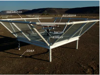
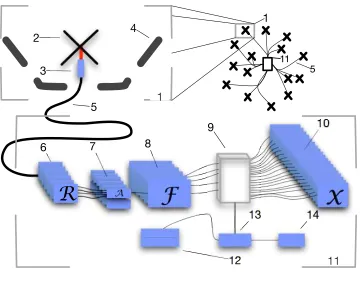
In Figure 2.2 we see a block diagram of the intentionally simple ”paper clips and a correlator” design. Crossed dipoles are mounted in matching ”crossed-trough” ground screens (see Fig. 2.1). Crossed dipole antennae are sandwiched between aluminum disks that act as a sleeve to broaden the frequency response to span 100 to 200MHz and a beam that is about 40◦wide at the half-power point and has its first null directed almost 180 degrees from zenith. A detailed model has been constructed using ”computer simulation technology” (CST) electromagnetic modeling software which includes the sleeve, reflector and ground plane (See Fig.2.3) and is used where necessary in this work.

Directly attached to the antenna is an ”active-balun” which provides 60dB of gain be-fore the unbalanced signal is transmitted over non-buried coaxial cable to a central RFI tight container. Inside the container the signal is amplified again, and filtered to the de-sired bandwidth. The resulting signal is digitized at 100MHz, Fourier transformed by an IBOB1 _{Field Programmable Gate Array (FPGA)-based ”F-engine” and distributed over a} commercial ethernet switch to a grid of FPGAs in the standardized ROACH2platform for cross-multiplication in an ”X-engine”.

Keeping the system low cost while simple to use and calibrate has been the focus of early design iterations. Single dipoles are used (in place of a phased array) to keep the frequency and sky variability of the primary beam to a minimum. The pre-amplifiers also act as baluns to low-cost unbalanced tv coax transmission lines. The second stage only

1_{Interconnect Break-Out Board}

(41)

antenna

balun

coax

reflector

sleeve

(42)

2 5 3 4 5 1 11 55 55 55 55 55 55 55 55 55 55₅ 5₅

F

_X

6 8 10 9 12 13 14 1 4 4 4 4 7

R

A 11

1. Dual polarization receiving element, 2. linear crossed broadband dipole, 3. amplifying balun,

4. square trough reflector,

5. TV coax cable (above ground), 6. filter and amplifier,

7. Quad - Analog to Digital Converter (ADC)

8. IBOB Fourier Transform Engine,

9. 10Ge ethernet switch performing ”few-to-many,N toN2_operation” 10. ROACH cross-multiply engine, 11. RFI tight 40’ container,

12. RAID storage, 13. Data receiving server, 14. Visualization,

The Epoch of Reionization: Foregrounds and Calibration With Paper

University of Pennsylvania

ScholarlyCommons

The Epoch of Reionization: Foregrounds and

Calibration With Paper

Daniel C. Jacobs

The Epoch of Reionization: Foregrounds and Calibration With Paper

ABSTRACT

Contents

List of Tables

List of Figures

Preface

Chapter 1

The Epoch of Reionization

1.1

In the beginning...

1.2

Observing the EoR

1.3

Theory

1.4

High z HI observing

1.4.1

Comparison to CMB

1.4.2

The Fourier Domain

[

mK

]

fractional delay [

]

[Mpc

]

P(k) [mK Mpc^3]

1.4.3

Noise Power Spectrum

1.4.4

SNR

|u|

k

ν

!

k

ν

k

B

≈

80M

Hz

1.4.5

Foreground Power Spectrum

1.4.6

Foreground Observations

1.5

Conclusion

Chapter 2

PAPER

2.1

Design

antenna

balun

coax

F

X

R

_X