Noise Reduction
in
Nonlinear Time Series Analysis
Mike Davies
Centre for Nonlinear Dynamics
University College London
September 1993
ProQuest Number: 10017775
All rights reserved
INFORMATION TO ALL USERS
The quality of this reproduction is dependent upon the quality of the copy submitted.
In the unlikely event that the author did not send a complete manuscript and there are missing pages, these will be noted. Also, if material had to be removed,
a note will indicate the deletion.
uest.
ProQuest 10017775
Published by ProQuest LLC(2016). Copyright of the Dissertation is held by the Author.
All rights reserved.
This work is protected against unauthorized copying under Title 17, United States Code. Microform Edition © ProQuest LLC.
ProQuest LLC
789 East Eisenhower Parkway P.O. Box 1346
Abstract
Over the last decade a variety o f new techniques for the treatment o f chaotic time series has been developed. Initially these concentrated on the characterisation o f chaotic time series but attention soon focused on the possibility o f predicting the short term behaviour o f such time series and we begin by reviewing the work in this area. This in turn has lead to a growing interest in more sophisticated signal processing tools based on dynamical systems theory. In this thesis we concentrate on the problem o f removing low amplitude noise from an underlying deterministic signal. Recently there has been a number o f algorithms proposed to tackle this problem. Originally these assumed that the dynamics were known a priori. One problem with such algorithms is that they appear to be unstable in the presence of homoclinic tangencies.
We review the original work on noise reduction and show that the problem can be viewed as a root-finding problem. This allows us to construct an upper bound on the condition number for the relevant Jacobian matrix, in the presence o f homoclinic tangencies. Alternatively the problem can be viewed as a minimisation task. In this case simple algorithm such as a gradient descent algorithm or a Levenberg-Marquardt algorithm can be using to efficiently reduce noise. Furthermore these do not necessarily become unstable in the presence o f tangencies. The minimisation approach also allows us to compare a variety o f ad hoc methods that have recently been proposed to reduce noise. Mzmy o f these can be shown to be equivalent to the gradient descent algorithm.
ACKNOWLEDGEMENTS
CONTENTS
Introduction
1. Preliminaries 10
1.1 State Space Models and Dynamical Systems 10
1.2 Stability o f Solutions 11
1.3 Lyapunov Exponents 12
1.3.1 Calculating Lyapunov Exponents 15
2. State Space Reconstruction 17
2.1 Motivation 17
2.2 Takens’ Embedding Theorem 18
2.3 Linear Filters and Embedding 22
2.3.1 FIR Filters 22
2.3 .2 HR Filters 23
2.3.3 Singular Systems Analysis 24
2.4 System Identification 27
2.4.1 Mutual Information 31
2.4.2 Predictability Criteria 32
2.4.3 Further Optimisation 35
2.5 Function Approximation 35
2.5.1 Interpolation, Extrapolation and Approximation 36
2.5 .2 Global Function Approximation 37
2.5.3 Local Function Approximation 41
3. Noise Reduction: Theory 45
3.1 Pseudo-Orbits and Shadowing 46
3.2 2^ro-finding and the Shadowing Problem 53
3.2.1 Manifold Decomposition 55
3.2.2 Approximation o f the Stable and Unstable Manifolds 56
3.2.3 Tangencies Imply ill-conditioning o f D 58
3.2.4 Solution by SVD 60
3.3 Implicit and Explicit Shadowing 62
3.4 Minimising Noise and Weak Shadowing 66
3.4.1 Solution by Gradient Descent 67
3.4.2 A Comparison with Other Methods 69
3.4.3 Solution by Levenberg-Marquardt 72
3.4.4 Other Minimisation Methods 76
3.4.5 Exact Shadowing in the Hyperbolic case 76
3.5 A Worked Example 78
4. Function Approximation for Noise Reduction 86
4.1 Shadowing Nearby Maps 87
4.2 Estimating the Dynamics 90
4.2.1 Alternating Noise Reduction and Dynamics Estimation 91
4 .2.2 An Extended Levenberg-Marquardt Algorithm 95
4.3 Explicit Shadowing 99
4.3.1 An Extended Manifold Decomposition Algorithm 101 4 .3.2 Explicit Shadowing and the Restricted Step Method 104
5. Noise Reduction: Numerical Properties 109
5.1 End Effects and Error Propagation 110
5.2 Convergence o f Zero Dynamic Error 113
5.3 Improvements in Signal-to-Noise Ratio 117
6. Noise Reduction: Applications. 119
6.1 Noise Reduction Applied to the Lorenz System 120
6.1.1 Data from a Chaotic Attractor 121
6.1.2 Data from a Periodic Orbit 125
6.1.3 A Comparison with Linear Filtering 128
6.2 Signal Separation 133
6.3 Improved Deterministic Modelling: Experimental Laser Data 134
7. Conclusions 141
Introduction
Our aim in this thesis is to develop a theory for methods o f reducing low amplitude noise from an underlying deterministic time series. For our purposes we can define a time series as a sequence o f observations that are a function o f time. Furthermore we only consider discrete time series and whenever examining continuous time series we will convert it into a discrete form by sampling it at a finite rate.
Traditional time series analysis is not new and many signal processing tools, including noise reduction techniques, have been developed based on such analysis. However traditional methods (FFT, ARMA, etc...) are, in general, restricted to linear transformations. This means that noise reduction techniques often involve identifying regions o f the frequency domain where the desired signal predominantly lies. However the performance o f such spectral methods is inevitably restricted if the noise is broad band.
A better approach would be to try to identify a discriminator that completely distinguishes between the wanted signal and the noise. Here we develop such an approach using low dimensional determinism to separate the two signals. This would not make a particularly interesting discriminator if we limited ourselves to traditional linear models since the resultant time series would merely have a number o f discrete spikes in its frequency spectrum. However the same is not true for nonlinear models and possibly one o f the most important lessons to be drawn from the study o f nonlinear dynamics is that an apparently random signal, from a traditional statistical viewpoint, can be generated by a simple nonlinear deterministic system. Such signals are termed ‘chaotic’ and generally have broad band frequency spectra. Thus standard spectral methods for noise reduction are not directly applicable. This, and the recent growth in the study o f experimental chaotic systems have led to a demand for good noise reduction techniques for such systems based on dynamical systems theory. It is this problem that we aim to address here.
single scalar time series. For this purpose we include a discussion on the important result o f Takens’ embedding theorem which demonstrates that, under suitable constraints, such equivalent state spaces exists and can be used approximate the dynamics and therefore to predict the short term furture behaviour o f the time series.
We can then use these methods to construct various procedures o f noise reduction. Initially we describe the noise reduction methods that are based loosely on the shadowing lemma. The shadowing problem can then interpreted as a rank deficient root-finding problem. In this context a noise reduction algorithm that has been proposed by Hammel can be seen as applying a set o f reasonable constraints to the problem to make it full rank. However we demonstrate that even with these additional constraints the problem becomes ill-conditioned when the embedded trajectory becomes close to a homoclinic tangency. We then show that the problem can be reformulated as a minimisation task. This allows us to treat tangencies in a more stable manner by using either a gradient descent or a Levenberg-Marquardt minimisation procedure. It also provides us with a framework in which we can compare various other noise reduction schemes that have been proposed.
In chapter 4 we go on to extend these ideas to include the problem o f modelling the dynamics within the noise reduction algorithm. This makes sense since both procedures aim to minimise the same approximation errors. We compare this approach to modelling the dynamics and reducing the noise separately. Our results show that intergrating the two steps together makes the noise reduction both more stable and more accurate.
1. Preliminaries
This chapter contains some o f the basic definitions and concepts that are required in studying nonlinear dynamical systems. We have made no attempt to make this section complete and we have concentrated on the ideas that are specifically used in subsequent chapters. In section 1.1 we introduce definitions for continuous and discrete time dynamical systems. Then we discuss the possible solutions for such systems along with their stability properties. Here we include a definition o f the important class o f hyperbolic sets. Finally we define the Lyapunov exponents and explain how they gives us information about the stability o f a solution. We also discuss a method for calculating these exponents for a given orbit since we will need to use this in chapter 3.
1.1 State Space Models and Dynamical Systems
We define a dynamical system as a map or vector field on some finite dimensional manifold M (usually compact) such that either (continuous time):
^ =/(AT(/)) , / € E (1.1.1)
where x(t) is a point on the d dimensional manifold A/, or (discrete time):
= / ( ^ , - |) . « e N (1.1.2)
where, again E M. We will also require in both cases that the dynamical system ,/, is to some extent smooth (i.e. to have continuous derivatives to some order). For a discussion o f the existence and uniqueness o f solutions for such systems see, for example, Guckenheimer and Holmes [1983]. The manifold M on which the dynamics acts is then called the state space (it is also referred to in some texts as the phase space) and knowledge o f the position o f a point in state space defines a unique solution with respect to the dynamics.
manifold. This concept has been greatly enhanced in recent years by the work on the existence o f inertial manifolds (see Constantin et al [1989] or Temam [1988]).
1.2 Stability of Solutions
We can now consider the solutions for such systems and their stability. We are particularly interested in some concept o f ‘steady state’ solutions. For example, one simple steady state solution o f equation 1.1.2 is a periodic point, which is a point, x, where there exists an n such that/"(xj = x. The stability o f a periodic point can then be evaluated from the eigenvalues o f the derivative o f the function at this point: %. This can be divided into stable and unstable subspaces. Solutions on the linear subspace, spanned by the stable eigenvalues, whose moduli || X || < 7 , will contract onto the fixed point at an exponential rate. Similarly points on the subspace, E /, spanned by the unstable eigenvalues (|| X || > 7) will diverge away from the fixed point at an exponential rate.
However one o f the interesting features o f nonlinear dynamics is that complex aperiodic steady state motion is possible and we would like to be able to extend the idea o f stability to more general invariant sets. An important concept in this respect is that o f hyperbolicity. We take the following definition from Shub [1986]:
Definition: We say that A is a hyperbolic set for a map f:M ^ M if there is a continuous splitting o f the tangent bundle o f M restricted to A, TM^, which is Tjf invariant:
TM^ = 0 E “; Tf{E^) = E'; 7/(E “) = E “ (1.2.1)
and there are constants c > 0 and 0 < X < 7, such that:
||37"|j.| < c r , niO
q 2 2)
Here the linear subspaces and E “ can be considered to be generalisations o f the stable and unstable eigenspaces o f % for the periodic case.
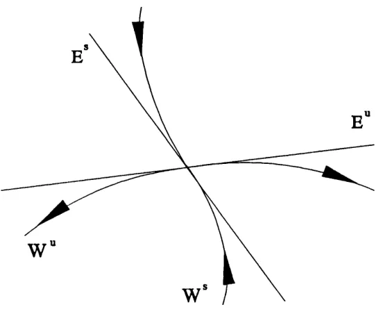
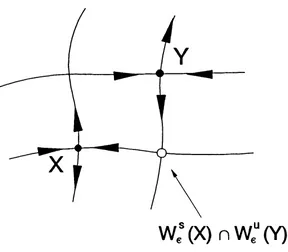
Finally we can extend these stability concepts from the infinitesimal to the local. Here we define the local stable and unstable manifolds in the e neighbourhood o f a point, x, in a hyperbolic set as follows:
K ( x f ) = tv I
d ( f \ x ) J ^ i y ) )
^ 0 as /I ^ + 0 0 (1.2.3)and
(y)) < e, V«>0}
= tv E M I #"(% ),/"Cv))
0
as n ^ -0 0 (1.2.4)and d ( f \ x ) J ' ^
(y)) <e, V/z<0}
These can be related to the linear sub spaces discussed above by the stable manifold theorem (see Shub [1986] for a definition and proof) which states that these local manifolds have the same dimension as, and are tangential to their linear counterparts and £ “. This idea is illustrated in figure 1.2.1.
Thus, if a set is hyperbolic, we know that in the neighbourhood o f this set the solutions to the associated nonlinear map behave in a qualitatively similar way to the solutions in the linearised system. This is important when considering the properties o f solutions close to a hyperbolic set and we will specifically use these ideas when discussing the shadowing problem in chapter 3.
1.3 Lyapunov Exponents
Définition: Let f:M -» M and x E. M. Suppose there exist nested subspaces in the tangent space Tfi at f '( x ) such that
R" = D D ... D and the following holds:
(1) Tf(E/») =
(2) dim E P = n + 1 - j
(3) l i m ^ In ( I / N ) \ [ ( T f f a ' f n ' ^ . v \ \ = h ’ ^ v € Then the set \ j are the Lyapunov exponents o f / a t x .
It is clear from this definition that if jc is a periodic point then there is a strong relationship between the Lyapunov exponents and the eigenvalues o f the tangent map Tfi. Indeed the Lyapunov exponents are simply the logarithm o f the moduli o f the eigenvalues. However the importance of the Lyapunov exponents stems from the fact that they are also applicable to aperiodic solutions such as chaotic attractors.
The concept o f Lyapunov exponents can be extended to general invariant sets if we assume that the set possesses an invariant probability measure (i.e. one that is invariant under the action o f f) and that this probability measure is ergodic (essentially that time averages equal spatial averages). We can then make use o f the remarkable theorem of Oseledec [1968]:
Theorem (Eckmann and Ruelle [1985]): Let p be a probability measure on a space M,
and f:M M a measure preserving map such that p is ergodic. Let T:M the m x m
matrices be a measurable map such that
j p{dx)\og* II T{x) II < oo (1.3.1)
where log^ u = max(0,log u). Define the matrix 7 ” = T(f'''^x)...T(fic)T(x). Then, fo r p-almost all x, the following limit exists:
M 2n
Urn ((7;)^(7r)) = (1.3.2)
everywhere with respect to the invariant measure. A more detailed discussion o f this theorem and a proof are given in Johnson, Palmer and Sell [1989].
Physically we can interpret the Lyapunov exponents as a measure o f the sensitive dependence upon initial conditions. That is, the rate o f exponential growth o f an infinitesimal vector is given, in general, by the largest Lyapunov exponent. Similarly the exponential expansion o f an infinitesimal ^-dimensional surface is given by the sum of the largest k Lyapunov exponents. Note that this means that, if the system is dissipative then the sum o f the Lyapunov exponents must be negative.
1.3.1 Calculating Lyapunov Exponents
Finally we consider how we could calculate the Lyapunov exponents for an attractor, given a fiducial trajectory from the system. Here we make use o f the physical interpretation described above. That is we know that a vector chosen in the tangent space will, in general, align itself with the most expanding direction under the action o f T p. It will then asymptotically expand at the rate defined by the largest Lyapunov exponent. Similarly an k-dimensional linear subspace chose in the tangent space, under the action of Tjf”, will align itself with the k-dimensional subspace associated with the k largest Lyapunov exponents.
Hence we need to identify such nested subspaces from a fiducial trajectory. One method for doing this is to decompose T f in terms o f % (the derivative o f / a t the iih point in the trajectory) in the following way (see Eckmann and Ruelle [1985]):
Tf,Q,
== Q2^2^
(1.3.3)
T f n Q n - \ = Q n K '
7T Ô„= Ô, n
i*rt
Thus if we choose Qq to be the identity matrix this method provides a stable method for decomposing Tf" into an orthonormal matrix and an upper triangular matrix (the product o f upper triangular matrices is upper triangular). Thus the kih diagonal element o f the product o f upper triangular matrices provides information about the expansion o f the direction in the ^-dimensional linear subspace spanned by the first k vectors in Qq that is orthogonal to the k-1 dimensional subspace spanned by the first k~l vectors in Qq. Finally, since the diagonal elements o f the product o f upper triangular matrices are merely the product o f the individual diagonal elements we can obtain an estimate for the Mh Lyapunov exponent as:
IS ,=i
2.
State Space Reconstruction
So far we have considered the modelling of dynamical systems in a state space. However in an experimental environment it may not be possible to measure all the variables to produce a state space. Indeed it may not be obvious what the actual state space is. It is therefore useful to consider how much information from a system is required to allow an adequate model to be constructed. This chapter reviews the work that has been done in this area with respect to modelling dynamics from one, or a few, scalar time series. The most important result here is Takens’ embedding theorem which provides the basis for all the other methods discussed in this chapter. However before considering the theory in detail the motivation for the problem is set out.
2.1 Motivation
We have already mentioned that finite dimensional dynamical systems can be studied by constructing their state spaces, such that each point in the state space can be uniquely identified with a possible state o f the physical system. This, and the knowledge o f the dynamics, provides us with the ability to predict the future state o f the system due to the uniqueness o f the solutions for any given state. Our aim is to achieve something similar when faced with a time series measured from some dynamical system.
This is essentially the idea behind state space reconstruction. We are trying to construct a state space that is observable from the time series. This space therefore must reproduce the original state space under a smooth transformation, in some way. Then, if we can associate a point in the time series to a uniquely point in our reconstructed space, the dynamics can be realised by a map that takes these states to the next associated state in time.
reconstructed space. Takens’ embedding theorem demonstrates that it is possible to construct such a state space, thus opening up a whole host o f opportunities for identification and prediction o f time series from experimental dynamical systems.
2.2 Takens’ embedding theorem.
Takens’ observed that the effect o f the dynamics on the time series provides us with enough information with which to reconstruct a space that contains a submanifold equivalent to the manifold on which the original dynamics acted. The proposed space is constructed using "delay coordinates", which are defined by a ^/-dimensional vector of the form:
{y(x ), y{<t>{x)), y{<l>‘‘' \ x ) ) ]
where % E M is a point in the manifold Af on which the mapping function (t)(x) : M M acts and y is the real valued function by which the dynamical system has been observed. If the dynamical system under consideration is continuous in time we can regard <t>(x) to be the time t map such that x(t-\-T) = 4>(x(t)).
Loosely speaking Takens’ theorem shows that ‘typically’, as long as the dimension o f the delay space is large enough, we have created a mapping from the manifold M into the delay space that is an embedding, where an embedding is defined as follows:
Definition'. Let f:M -* TV be a smooth map. We say that / is an immersion if the tangent map D f is one-to-one everywhere. We say t h a t /is an embedding if it is an immersion and everywhere one-to-one.
a.
b.
>
Finally the term ‘typical’ here means that this property is generic in the space o f mapping functions and observables. Here we will use this to mean that the subset for which the property holds forms an open set that is dense within the relevant space (conversely this means the set where the property is not satisfied is closed and nowhere dense).
The strict statement o f the theorem is as follows:
(Takens 1981) Let M be a compact manifold o f dimension m. For pairs (4>,y), <b: M -^ M
a smooth diffeomorphism and y:M R a smooth function. It is a generic property that
the map ^(4>,y):M defined by:
= (y(x), y{4>{x)), ..., y(<i>^(x)) ^ X e M
is an embedding (smooth is at least C^).
Sketch of Proof.
The proof o f Takens’ theorem follows closely to that o f Whitney’s embedding theorem (see Brocker and Janich [1982] or Hirsch [1976]). However some additional work is required since the ^ is not a typical mapping function. We briefly discuss the method of the proof.
Initially we impose some restrictions upon <^. We assume that there is a finite number o f points X 6 the set o f periodic points in M with period less than 2m+ 7 and that the eigenvalues o f are all distinct for x E 7^2^ o f period k. These restrictions are acceptable since they are generic properties o f 0 . We further assume that y maps all the points in 7^2^ onto distinct points in R. Finally we now note that both immersions and embeddings are open in the set o f all mappings. Hence we only need to show that the set o f (<f),y) for which ^ is an embedding is dense.
the derivatives dÿ,, dy(^^,..,dy4>^ span the tangent space TM^ for x E A detailed description o f how to do this is given in Noakes [1991]. Thus for the map associated with the adjusted y there is a neighbourhood V o f such that y is an immersion and locally an embedding.
We can now consider the points contained \n M \ V. First we construct a finite open cover on M \ V, { U j and a compact cover { K j such that C Î7, (some extra conditions also have to be imposed on {U j: see Takens’ [1981]). We can then show that y can be perturbed to ensure ^ 11, restricted to some f/ is an immersion on a closed set K C U. This can be done by following the immersion proof in Brocker and Janich [1982]. Hence for any we can adjust y to immerse K^. To make this property global we can then apply it individually to each open set, U^, in turn composed with a suitable bump function whose support is contained in L/,. Since the set o f immersions is open we can always choose the adjustment to make 4» | ^ an immersion on so small that our previous work is not destroyed.
Once 4» has been made an immersion on M, we can produce a new open cover { U j such that each is so small that $ | i s an embedding. Thus we only need to show that we can perturb y so that [(/, O 0 |yj = 0 for i ^ j . Again we can follow the embedding theorem in Brocker and Janich [1982] and the global results can be constructed in the same manner as above. This means that we can perturb y so that it one-to-one on M as well as being an immersion. Hence 4» for the perturbed y is an embedding.
2.3 Linear Filters and Embedding
It is worth considering the extensions o f Takens’ embedding theorem beyond delay embeddings to more general reconstructed spaces. One obvious candidate for an embedding space is linearly filtered time series. Often, intentionally or otherwise, the experimentalist’s data will have already been filtered when it is analyzed, therefore it is necessary to ask whether a reconstructed space can be made from this data. The two types o f linear filters described here are called Finite Impulse Response (FIR) filters and Infinite Impulse Response (HR) filters. An FIR filter is one with the following structure:
y . = Y , 7=0
where Uj are the constants o f the filter and y, is the time series resulting from filtering An HR filter has an additional relation to the past values o f y,:
7=0 *=1
where b,, are additional constants for the HR filter. There are also acausal filters where the value o f y, is determined from data in the future as well as the past, but they are not considered here.
It is important to distinguish between these two types o f filters since an FIR filter has only a limited "memory" o f past data whereas an HR filter, because it is recursive in nature, has a response that typically decays exponentially with time. This, it will be shown can lead to problems when filtering chaotic data. However first we should address the problem o f FIR filters.
2.3.1 FIR Filters
Theorem; Let V be a time series o f measurements made on a dynamical system (<t>,M), which satisfies the hypotheses o f Takens* theorem. Then f o r triples (a,<f>,v), where a =
(ao,aj,..aJ are the constants o f an FIR filter, it is a generic property that the method o f
delays, which constructs, from the time series U, vectors o f the form :
(Uj,Uj.i,...,Uj.i+i) where I > 2m I and Uj = a.Vj with finite n, gives an embedding o f M.
The proof o f this theorem follows closely to that o f Takens’ original theorem. However it is possible to interpret this reconstructed space as a linear projection from a delay space o f dimension l-\-n-l to a new space o f dimension I. Thus it is necessary to consider whether this projection destroys either uniqueness or differentiability. Broomhead et al showed that generically these properties were preserved if / > 2m -\-l.
2.3.2 HR Filters
Unfortunately it is not possible to produce a similar theorem for HR filters. This is because HR filters are recursive in nature and therefore possess their own dynamics. Farmer, Ott and Yorke [1983] studied a one dimensional linear system that was driven by an observable from the cat map:
yi
=
(2.3.3)
where y, is the output o f the linear filter, a is the contraction rate o f the linear system, and Zi is the observable from the cat map. They noted that the torus o f the original cat map when viewed in the extended dynamical system (that is including the linear system) ceased to be smooth when || a || > X. (the smallest Lyapunov exponent o f the cat map).
j'i = s (2.3.4)
J-o
where || a || < 1 and h ( x ± ) is the observation o f the state variable x ± . Then we can regard the filtering as part o f the observation process. That is, instead o f using the observation function in Takens’ theorem h ( x ), we observe the system via g ( x ) , g ; M- * R,
where y ± = g ( x ± ). Then we can consider whether g ( x ) satisfies the requirements for Takens’ theorem to hold. In particular we are interested in the smoothness o f the function, g ( x ) .
Consider a fixed point, p , o f the observed dynamical system p = f ( p ). Then we can write the partial differential of g ( p ) along the direction o f the eigenvector v associated with the smallest eigenvalue, y o f D f p .
M s l \ = V g> I o r H (2.3.5)
dx ^ dx ''
but, by our choice o f v, we know that D f~^ | , = 1 / . Thus for the partial derivative of
g ( x ) I, to remain bounded at p requires || a / y || < I . This means that the delay map based on g ( x ) will not be immersive at p. Furthermore, although g ( x ) may still be small perturbations io g ( x ) will not improve the situation. This is because, by the definition of the HR filter, we are constrained to a very particular set o f observation functions. Thus if II a / y II > I there will be at least one point on the manifold that is not emmbedded. This may be more severe than results based on the smallest Lyapunov exponent and we should really consider the Lyapunov exponents o f every invariant measure on the attractor to ensure that the reconstructed manifold is smooth.
2.3.3 Singular System Analysis
effectively uses a bank o f orthogonal FIR filters for the reconstructed space. It is based on the trajectory matrix formed from the data set using the method o f delays. First the data must be organised into vectors or ’windows’ o f a certain length. Then the matrix takes the following form:
X =
(2.3.6)
where m is the window length. The trajectory is thus made up o f m-windows o f the data. We can now construct basis vectors in the m-window that are linearly independent with respect to the time series. This is done by diagonalising the covariance matrix X^X using eigen-decomposition :
XX'^
= V
52
(2.3.7)
Where is a diagonal matrix containing the eigenvalues o f X^X and V is the matrix whose columns are the eigenvectors associated with 5"^. Since the covariance matrix is the product o f X^ and X it can be shown that it is symmetric and positive semi-definite. Thus the eigenvalues are all positive and the eigenvectors are mutually orthogonal. We can now define m new time series that are linearly independent by rotating the trajectory matrix X with V to get XV. These new directions are the principal directions in which the data lies and the eigenvalues define the extent to which the data lies in the associated direction. These are also called the principal values. S and Vcan also be calculated from the singular value decomposition of the trajectory matrix, X = VSV^.
distinct sets by considering the effects o f noise. In such a situation, it is likely that some o f the principal values o f the trajectory matrix will be small since, if the window length is chosen to be such that its time span < 2ir/w where w is the band limiting frequency, the principal values will drop off quickly. Then the data will lie predominantly in linear subspace associated with the first few principal values. This can be seen as the redundancy o f over-sampling.
We can now divide the simple delay space into linear subspaces that do and do not predominantly contain the embedded data by considering the effect o f any additive noise. If the signal is corrupted by white noise then the covariance matrix will take the following form:
2 = 2 +
(2.3.8)
where I is the identity matrix and e is the variance o f the additive noise. The new principal values are simply modified by:
0^ = Ô? +
(2.3.9)
The space can then be divided into two parts. The sub space with principal values that are very much greater than and the subspace with singular values approximately equal to e^. We can now consider the data projected into the first principal directions to be approximately deterministic. These can be considered the best directions in the sense that they have maximum variance and hence maximum signal-to-noise ratio. However the number o f dominant principal values has no relationship with the embedding dimension o f the data. This is clear since raising the noise level will reduce the number o f dominant principal values whereas reducing it will increase their number, independent o f the true embedding dimension.
tends to zero).
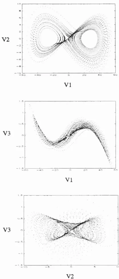
To illustrate this form o f embedding we took a 5000 point time series from the Lorenz equations, using a delay window o f length 10. The differential equations are:
^ = a (Y - X ) at
— = r X - Y - XZ (2.3.10)
dt
— = - b Z + X Y dt
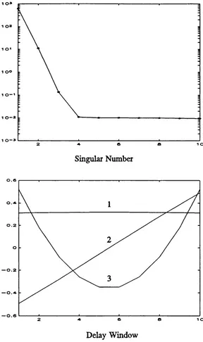
where a = 10, b = 8/3 and r = 28. The equations were integrated using a Runge-Kutta fixed step integration routine with a step size o f 0.001. After the transients had died down a time series o f 5000 points was obtained. The time series was then corrupted with 1 % additive white noise. The top picture in figure 2.3.1 shows the plot o f the normalised eigenvalues for the covariance matrix using a delay window o f 10 points. It is clear from the figure that the singular values can easily be divided into the first three that are above the noise floor and the others.
The first three associated principal directions are also shown in figure 2.3.1 and there is obviously a strong resemblance between these basis functions and the first three Legendre polynomials. The projections o f the delay space into the associated principal directions are shown in figure 2.3.2.
2.4 System Identification
1 o»
1 o*
1 o®
2 6 S 1 O
Singular Number
0.6
0. 2
— 0 . 2
— 0.4
-— 0.6
2 4 6 8 1 O
Delay Window
Figure 2.3.1: The top picture shows a plot o f the
V2
VI
V3
VI
V3
V2
(i.e. what dimension and delay vectors to use).
It has previously been stated, [Kennel et al 1992], that the problem o f choosing an embedding dimension and the problem o f choosing delay time (the latter can be generalised to the choice o f any linear filtered state space) are independent since the former is a geometric problem and the latter is a statistical problem, however this is not the case. Even when the ideal situation o f no noise and infinite data length is considered it can be shown that delay times and dimension choice are linked. Although Takens’ theorem states that the data will generically be embedded when the embedding dimension, d^, is greater than 2m + 7 it is commonly known that many data sets can be embedded in lower dimensional spaces (Whitney showed that there always exists an embedding o f an m-dimensional manifold in 2m dimensions: see, for example Sauer et al [1992]). Thus for many data sets there are open sets o f the pairs {4>,y} for which the manifold containing the data is embedded in a reconstructed space for < 2m + L However a corollary to Takens’ theorem is that for d^ < 2m 4-7 the space o f the pairs {<t>,y} will always contain open sets for which the manifold is not embedded and the dimension of the bad set in these cases is 2m-(7g. These can easily be found by choosing an observation function such that two parts o f the manifold are mapped into the same local neighbourhood in the state space then generically the intersection o f the two local parts o f the manifold will be 2m-(7g. Therefore it may be possible to have an embedding for one choice o f delay space for d^ < 2m 4-7 whereas another choice o f delay space may require d^ = 2m + 1 before an embedding is possible. The problem becomes even less well defined when finite noise levels are considered.
2.4.1 Mutual Information
Shaw [1985] proposed using the concepts o f mutual information to achieve an optimal embedding and this idea was taken up by Fraser and Swinney [1986] and Fraser [1989], where they argued that the choice o f dimension and vectors used in singular systems analysis was intrinsically linear, whereas optimal choices o f coordinates should be based on nonlinear criteria. It was proposed that minimising the mutual information between coordinates would provide coordinates that were most independent and therefore in some sense optimal. The mutual information between two variables %, and y is U^>y) = - fi(x \y ) where H (x\y) is the entropy associated with the conditional probability o f x given y . Thus it measures how much information y provides about the variable x. Unfortunately this idea is flawed for two main reasons.
First o f all a chaotic attractor has positive entropy and therefore creates information. This means that as the delay time, t, tends to infinity the mutual information between x(t) and
x(t-¥T) tends to zero: this is obviously not optimal! To overcome this problem Fraser suggested choosing the first local minimum. However the mutual information function may not always have a minimum. In fact, it is quite common in maps for the mutual information function to monotonically decrease with r since the positive entropy is the dominating factor.
The main problem o f this method is the heuristic idea that maximum information will be gained about the state space by choosing a variable that is most independent from the previously chosen variables. This is not necessarily true and it would be a more justifiable approach to explicitly aim to maximise the information about the state (this was the idea originally proposed by Shaw).
intend to approximate the dynamics in the state space with a method that requires the variance o f the probability distribution to be small (this is essentially the case when we aim to construct a one-to-one map). Therefore we favour the use o f predictability criteria.
2.4.2 Predictability Criteria
In this section we discuss error estimates as criteria for estimating when the data has been successfully embedded. The main idea is that an error function provides a good measure o f how well the embedding can be considered to possess a one-to-one mapping from the embedded data onto itself. This method has been implemented in a variety o f different forms: Aleksic [1991], Savit and Green [1991], Cenys and Pyragas [1988], Kennel et al [1992] and Sugihara and May [1990]. Although these methods are similar their implementations and the interpretations given to the methodology vary significantly. Some o f the interpretations are geometric in nature. Others are more statistical.
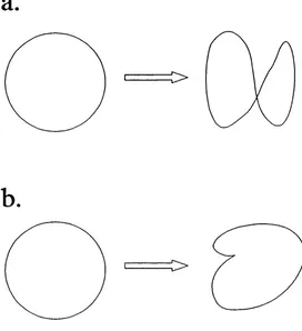
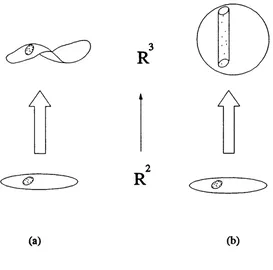
The main idea o f the above papers is based on local techniques although there appears to be no reason why this cannot be extended to global descriptions o f the embedding (see the end o f this section). The method depends on the effect o f increasing the embedding dimension on nearby points. If the data is fully embedded in some reconstructed space o f dimension d then the addition o f an extra state variable will create a new space in of dimension d-\-l 'm which the data will also be embedded. Hence two close points will remain close in a higher dimensional space. This idea is illustrated pictorially in figure 2.4.1.
R
A
R
<2?(a) (b)
It should be noted that the closeness test may not itself be necessarily straight forward. For example the threshold criterion used in Kennel et al [1992] is:
rI
where is the distance between a point and its nearest neighbour in the rf-dimensional reconstructed space. However they noted that this criterion alone is not a satisfactory measure since, for finite data, as the dimension increases the distance between nearest neighbours tends to the span o f the data set in that dimension, hence the criterion above will tend to zero as the dimension, d, becomes large. To solve this problem Kennel et al introduced a second test to determine whether the distance o f nearest neighbours was too large to regard the data points as close.
We can see why this happens by considering the relation between R / and
R^+i^-where Ri^(Xd+],yd+j) is the distance between x and y in the new coordinate direction. Thus it is obvious that when R / becomes very large the test in equation 2.4.1 will fail to be o f use. However, if we only consider the size o f Ri^(Xa+i,yd+i), we automatically get around this problem.
Finally there is no reason why the predictability criterion cannot be extended to global descriptions o f the embedding. That is we could use the prediction error from a global function approximation for the dynamics (see section 2.5.2) as a measure to ascertain when the data has been embedded. Indeed, if our ultimate aim is to produce a predictive model for the data, it would seem that a good criterion for optimising our state space parameters would be the success o f our predictive model.
2,4.3 Further Optimisation
The methods described above construct embeddings by repeatedly choosing an additional delay vector that is optimal in some sense with respect to the present set o f state vectors, until the improvement is insignificant. However this does not necessarily optimise the whole space. To attempt to find such an optimal state we would need to search through the set o f all reconstructions that are to be considered. In this respect, Meyer and Packard [1992] have looked at determining local embeddings for high dimensional attractors. They used a predictability criterion to choose the optimal local embedding for a given point in a high dimensional attractor. Obviously this problem is going to be nonlinear and to obtain a good minimum a sophisticated minimisation technique is required. Meyer and Packard [1992] solve this by using a genetic algorithm. However, in general, if a global embedding is required the gains are unlikely to warrant the extra effort.
2.5 Function Approximation
Once the data has been embedded into a reconstructed space it is possible to estimate the dynamics that produced the time series. This can be done by approximating the function f:K^ ^ that maps the state space onto itself.
g:K^ -» R from the reconstructed space onto the real line such that g predicts the next point in the time series:
~
(2,5.1)
then the remainder o f the new point in the state space is defined by a simple shift in the delay window so that the new state vector is:
Î -
(2.5.2)
Once the dynamics have been modelled the system can be investigated further: e.g. prediction, control, filtering, etc...
2.5.1 Interpolation, Extrapolation and Approximation.
If the data is noise free and arbitrarily long then the dynamics will be uniquely defined on the embedded data set. However, in reality, a data set will always have a finite length. Therefore, in general we will not be able to ascertain a prediction directly from the data and it will be necessary to interpolate between data points. Also, in some cases, it may be useful, although more dangerous, to extrapolate from some data points. This requires us to select a subset o f the relevant function space since there are an infinite number o f functions that can be interpolated through any finite data set.
i=d
(2.5.3)
Although the least squared estimate is statistically based on quite strict assumptions about the nature o f the noise present it does, in general, provide a good estimate for function approximation even when some o f the assumptions are relaxed. This and the fact that it can often be solved directly makes it our preferred choice.
Finally we have to consider the choice o f the function set from which we intend to make our approximation. Unfortunately it is difficult to identify what defines a good approximation function and most o f the function forms used are, at best, based on weak ideas about the type o f functions that are good and, at worst, on historical accident. Although there are no real optimal methods some techniques have advantages over others. There are two main categories o f function approximation that have been applied to fitting nonlinear state space models. These are briefly discussed below.
2.5.2 Global Function Approximation
This approach restricts the approximation to a single set o f functions that can usually be defined by a parameter set, p . Since there are no rigorous arguments for choosing one function form over another the speed at which a solution can be obtained plays a major role in the type o f function forms that are used. In practice, this means that the function model should be chosen such that the parameters can be calculated directly which requires the model to be linear with respect to the parameters:
g(2) = 4).(x) (2.5.4)
i=l
We can see this by considering the error function in terms o f the weighting parameters:
* = E - E '* '; t / Ü ,)
i^d \ y=l
(2.5.5)
Because the function model is linear in parameters the error function is quadratic in parameter and has a unique minimum that can be calculated directly using linear algebra. Equation 2.5.5 can be rewritten in matrix form:
H = e^e = ( x - P w Y ( x - P w ) (2.5.6)
where e is the error vector for the time series, x is the vector o f points from the time series to be predicted and P is the design matrix that has the following form:
' <1>2^) ••• 4>^(^i) ' 4>2(^2) •••
P = (2.5.7)
whose i j element is the value o f theyth basis function at the /th state vector. We can now
solve for the minimum value o f H by differentiating and equating to zero:
ÈK
d w
= 2P ^ (x - Pw) = 0 (2.5.8)
Hence the values o f Wj that minimise the error are:
w = (P'^P)-^P^x (2.5.9)
useful when P is badly conditioned.
Thus we have shown that it is possible to reduce the approximation o f nonlinear functions to a simple linear problem that can be solved directly by matrix inversion. However this method requires that the function model is linear with respect to the weighting parameters. We will now discuss below some o f the function models that fit into this category:
Polynomials. Polynomial expansions are probably the most obvious choice o f function form and can easily be written as a linear sum:
g W = ÛQ + f l j i + + ^ 3 ^ ... (2.5.10)
However when the order o f the polynomial or the dimension o f the domain become large the number o f free parameters grows rapidly and will in general such fits are most useful when the order o f the polynomial can be kept small (for example in local function approximation). A better alternative is to use rational polynomials.
Rational Polynomials. These are a simple extension from the polynomial expansion. A rational polynomial is the ratio o f two polynomial expansions:
g(2) = 7 - ^ (2.5.11)
(1 + «)
where both p and q are polynomial expansions. The above equation is obviously not linear in parameters. However direct solutions can be obtained by minimising a slightly different error function (see Casdagli [1989] and the references therein):
/I* = E ( (1 * - P ( î ) f i=d
Radial Basis Functions. These provide an alternative global function fit that is not based on polynomial expansions. Radial basis functions are functions that are solely dependent upon some distance measure, usually Euclidean, from the basis function’s centre, c. Thus the global model takes the following form:
/ k ) = 5 3 ^ 1 4>(ll2E - CjN) (2.5.13)
i=l
where w, is the weight associated with the fth basis function. It can be seen that, as long as the centres are defined a priori, this model is linear in parameters and can therefore be solved directly.
Radial basis functions were initially introduced as a means o f performing multi dimensional function interpolation (see, for example, Powell [1985]). In this case the centres are automatically chosen as the data points themselves. The basic incentive in using radial basis functions is that they can exhibit good localisation properties. That is the value o f the resulting function at a point is mainly defined by nearby points in the space. In this sense radial basis functions are similar to the local methods described in the next section. They can also be shown to possess other desirable properties: see, for example Michelli [1986]. One example o f a radial basis function model is the basis function r^log r. If this basis set is applied in 3 dimensions it can be shown to be equivalent to interpolating the data with thin plate splines. Some other commonly used basis functions are: exp(kr), (r^ + -f and / . In each case ^ is an arbitrary scaling factor that has to be predefined.
Finally it is important to mention that there are methods o f nonlinear function approximation that are not linear in parameter, such as neural networks. However these methods require iterative procedures to minimise the error function and therefore the fitting procedure takes orders o f magnitude longer. For this reason we favour function approximations such as radial basis functions which appear to be able to achieve good fits without being computationally too costly.
2.5.3 Local Function Approximation
Another approach to function approximation is to construct local models. The incentive for this is that, if the surface to be approximated is quite complicated then a global approximations may perform poorly. However if we assume that the function is to some extent smooth we can exploit the local structure that this imposes. Consider the Taylor expansion o f a function/around a point in state space x:
fix + 6%) « fix) + b x ^ + bx^— bx + . . . (2.5.14)
^ dx dt^
Then we know that the function o f a small enough neighbourhood o f x is closely approximated by its Taylor expansion to some order. Thus, instead o f approximating the function globally, we can approximate the Taylor expansion locally.
To implement this method we need to define a metric with which to construct a neighbourhood o f the point we wish to predict. We then find all the points in the training set that lie in that neighbourhood and fit a local model over the neighbourhood in the same way that was described in the last section. The most natural function model to use when approximating a Taylor expansion is to use a simple polynomial expansion. Unlike global polynomial expansions, the order o f the polynomial can be kept small such that each individual fit is well behaved.
atmospheric forecasts. However the most popular method is to use local linear approximation (see, for example Farmer and Sidorowich [1987] and Sugihara and May [1990]). This also provides derivative information which is useful for calculating Lyapunov exponents and also for performing noise reduction (see chapter 3). Higher order polynomials have also been investigated by Farmer and Sidorowich [1988]. Although some improvement can be gained by increasing the order o f the polynomial this gain is likely to be limited by the size and accuracy o f the data set.
However we have so far not specified how to chose a neighbourhood. The most natural way is to chose all the data points that lie within a specific distance from the point, y, to be predicted. However it is not obvious what the distance should be or whether there will be enough points within the neighbourhood to make a good prediction. Hence another method for choosing a neighbourhood o f y is to find the k nearest data points to the y. This then guarantees that there will be enough points to make the approximation well defined. Finally a more systematic approach that has been used to define neighbourhoods in a different context was presented by Broomhead et al [1987] in calculating topological dimension o f attractors. They looked at the scaling o f the local prediction error with the neighbourhood size, a. When the scaling changes as then the neighbourhood is becoming too big. Therefore it should be possible to devise an algorithm to use the maximum possible neighbourhood before curvature errors become dominant.
Finally, once a mechanism for choosing neighbourhoods has been found and the type of local function approximation has been chosen, we need a method for efficiently searching through the data set to locate the nearest neighbours. If we were to use a simple sequential search we would soon find that the this type o f function approximation was too costly, since we would be spending all our time searching through the data set. However there are fast search algorithms available that speed up this process to an acceptable level. These generally involve partitioning the data in the state space and then ordering these regions in a manner that is easy to search. Two examples o f quick search algorithms that have been used in local function approximation are k-d trees and box-assisted algorithms. See Bentley and Friedman [1979] for a full comparison o f the various methods available.
functional form to be described by a parameter space. Although parameters are calculated for the functions in each neighbourhood this creates a vast number o f free parameters many o f which are unlikely to be independent. Thus it is not easy to consider a family o f functions related to perturbations o f the data set. Although this appears to be a small point we will show in chapter 4 that such a family o f functions can be used effectively to enhance the performance o f noise reduction algorithms.
2.6 Approximation Errors versus Measurement Noise
In the next chapter we will discuss methods by which the noise in the time series can be reduced. However before looking at these techniques it is necessary to consider how different types o f noise will effect the data in the reconstructed space. Broadly speaking, dynamical systems can be contaminated by two types o f noise;
Dynamic noise is a stochastic process within the dynamical system such that the actual trajectory is perturbed by the random process.
Measurement noise is a random component that corrupts the time series but does not effect the dynamics or the underlying trajectory.
We will restrict ourselves to additive dynamic noise and additive measurement noise, although in practice, noise does not have to take these forms.
3.
Noise Reduction: Theory
In this chapter we investigate methods o f reducing low amplitude noise from an underlying deterministic time series. At this stage we will assume that the data has already been embedded and that the dynamics are known a priori. Thus we have a ‘noisy’ trajectory that can be identified with some nonlinear dynamical system. To reduce the dynamic noise associated with the trajectory we aim to adjust the trajectory such that it is less noisy. This makes sense since the original trajectory can be interpreted as the new trajectory with additive measurement noise. Hence noise reduction, in this context, is a method o f transforming dynamic noise into measurement error.
The idea for noise reduction o f this type using state space methods was proposed by, among others, Kostelich and Yorke [1990]. Their method involved breaking the time series up into overlapping sections and adjusting these sections to make them more deterministic, while remaining ’close’ to the original sections o f the data. Unfortunately this does not provide a unique minimization process since it involves simultaneously minimizing the distance o f the new trajectory from the old one and the distance o f the data points from deterministic ones. Thus the cost function is a combination o f these two aims:
s = [ wj i - + II - a:, I + II f ( x ) - AT..., 1^ ] (3.0.1)
where f(x) is the local mapping function, is the original trajectory and x^ is the new ’cleaner’ trajectory. The weighting w between the two parts is arbitrary. This arbitrariness is intrinsic in the problem o f any noise reduction method and much o f the work in this chapter looks into ways o f solving this and other indeterminacies.
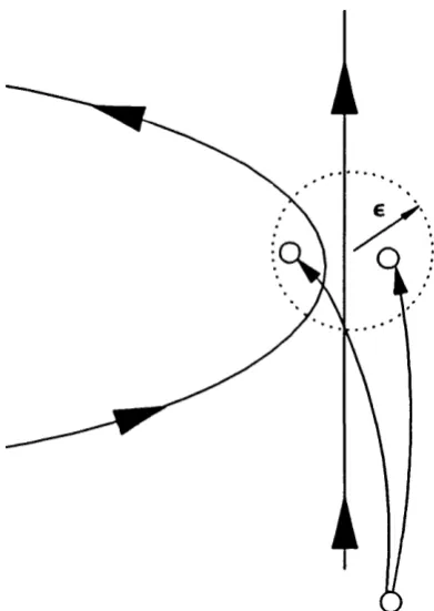
![Figure 3.4.1 : A graphical representation of the projection noise reduction method of Cawley and Hsu [1992] and Sauer [1992]](https://thumb-us.123doks.com/thumbv2/123dok_us/9159103.1453916/71.595.94.459.185.482/figure-graphical-representation-projection-reduction-method-cawley-sauer.webp)